Strong field dynamics with ultrashort electron wave packet replicas

Abstract

We investigate theoretically electron dynamics under a VUV attosecond pulse train which has a controlled phase delay with respect to an additional strong infrared laser field. Using the strong field approximation and the fact that the attosecond pulse is short compared to the excited electron dynamics, we arrive at a minimal analytical model for the kinetic energy distribution of the electron as well as the photon absorption probability as a function of the phase delay between the fields. We analyze the dynamics in terms of electron wave packet replicas created by the attosecond pulses. The absorption probability shows strong modulations as a function of the phase delay for VUV photons of energy comparable to the binding energy of the electron, while for higher photon energies the absorption probability does not depend on the delay, in line with the experimental observations for helium and argon, respectively.

1 Introduction

Technological advance has made it possible to expose atoms and molecules to a combination of attosecond pulse trains (APT) and infrared (IR) laser pulses with an accurate control of their phase delay [1]. The photo electron spectrum of atoms in this combined light field has been studied [2], as well as above threshold ionization [3], the latter together with high harmonic generation in the combined field also theoretically [4], along with another quasi-analytical formulation [5] and a fully numerical R-matrix calculation [6].

While many parameter combinations are possible, a dynamically very interesting regime emerges when the energy of the VUV photon from the APT is comparable to the ionization potential but the IR pulse alone (typically 780 nm wavelength) is not intense enough to ionize the atom. The combined action of both fields leads to a time-dependent wave packet dynamics which is very sensitive to the phase delay, equivalent to the carrier-envelope phase (CEP) of the IR field. Consequently stroboscopic measurements of interfering electron wave packets which overlap in this energy regime but leave in opposite directions have been demonstrated to provide a sensitive tool to measure phase differences [7]. In a subsequent experiment it has been recently shown that the phase delay does not only influence the photo electron spectrum, but also modulates the total ionization and absorption probability [8]. A solution of the one-electron time-dependent Schrödinger equation (TDSE) with a pseudo potential for helium yields excellent agreement with this experiment [8]. While quite generally interference of wave packets must be responsible for the pronounced oscillatory behavior of the absorption yield as a function of the phase delay, the exact reason and systematics of these oscillations is difficult to identify in a fully numerical solution.

Here, we formulate a minimal analytical approach. It elucidates the mechanism behind the pronounced structures in the electron observables as a function of phase delay in the spirit of the “simple man’s approach” successfully formulated for high harmonic generation in intense fields [9]. For a recent refinement of the simple man’s approach, see [10].

2 Ionization with an APT in the presence of an IR field: Analytical approach

We consider an electron bound with energy $\varepsilon_{\mathrm{i}}$ exposed to a train of attosecond pulses in one dimension. The intensity is so weak that we are in the single photon regime for each atto pulse of width $\sigma$ and central time $t_{n}$. Consequently we neglect the slowly varying envelope of the ATP and write for the interaction potential (in velocity gauge and rotating wave approximation)

$$V_{\mathrm{atto}}(t)=p\,\exp(-i\Omega t)\sum_{n=1}^{N_{\mathrm{atto}}}\exp[-(t-t_{n})^{2}/(2\sigma^{2})]\,,$$ (1)

where $p$ is the electron momentum and $\Omega$ the central frequency of the attosecond VUV pulses. The infrared field is characterized by the vector potential

$$A(t)=A_{0}\cos(\omega t+\varphi)\,.$$ (2)

It has linear polarization in the same direction as the atto pulses and a phase delay $\varphi$ with respect to the APT. Its envelope $A_{0}$ is assumed to be constant over the length of the APT. We use atomic units throughout the paper unless stated otherwise.

Since the APT gives only rise to single-photon absorption events, first-order time-dependent perturbation theory provides an accurate description under which an initial state $|\Psi(t_{\mathrm{i}})\rangle$ evolves into the state at time $t_{\mathrm{f}}$ according to

$$|\Psi(t_{\mathrm{f}})\rangle=-i\int_{t_{\mathrm{i}}}^{t_{\mathrm{f}}}{U}(t_{\mathrm{f}},t){V}_{\mathrm{atto}}(t){U}(t,t_{\mathrm{i}})|\Psi(t_{\mathrm{i}})\rangle\,dt$$ (3)

with the time evolution operators $U$ for the electron under the combined influence of the IR field and the Coulomb potential of the ion [14].

The key idea behind the simple man’s simplification which permits an analytical treatment is to consider the phases in the integral of Eq. (3) as the dominant contributions, $U_{\alpha}(t^{\prime\prime},t^{\prime})=\exp(i[\Phi_{\alpha}(t^{\prime\prime})-\Phi_{\alpha}(t^{\prime})])$, and to approximate the propagators before and after the photoabsorption differently, $U(t,t_{\mathrm{i}})\equiv U_{\mathrm{i}}$ and $U(t_{\mathrm{f}},t)\equiv U_{\mathrm{f}}$. Then, one gets from Eq. (3)

$$\psi(t)=\sum_{n}\int_{t_{\mathrm{i}}}^{t_{\mathrm{f}}}\exp{(\phi_{n}}(t))\,dt,$$ (4)

where the phase is given by

$$\phi_{n}(t;p,\varphi)=i[\Phi_{\mathrm{f}}(t_{\mathrm{f}})-\Phi_{\mathrm{f}}(t)]-(t-t_{n})^{2}/(2\sigma^{2})-i\Omega t+i[\Phi_{\mathrm{i}}(t)-\Phi_{\mathrm{i}}(t_{\mathrm{i}})].$$ (5)

Here, $\Phi_{\mathrm{i}}$ is the phase accumulated before the VUV absorption, where the electron remains in its initial state, almost unperturbed by the laser field. Hence, we may write $\Phi_{\mathrm{i}}(t)=-\varepsilon_{\mathrm{i}}t$, and define the energy $\varepsilon_{\mathrm{f}}=\varepsilon_{\mathrm{i}}+\Omega$ after the absorption of the VUV photon at time $t^{\prime}$. For $t>t^{\prime}$ we assume that the electron dominantly feels the IR field, described by the corresponding classical action (or, equivalently, quantum Volkov propagator)

$$\Phi_{\mathrm{f}}(t;p,\varphi)=-\int^{t}(p+A_{0}\cos(\omega\tau{+}\varphi))^{2}/2\,d\tau.$$ (6)

A wavefunction expressed as an integral over time with two phases $\Phi_{\mathrm{i},\mathrm{f}}$, as in Eq. (4), appears also in the analytical description of high harmonic generation, see e. g. Eq. (22) in [11]. In this context, often a stationary phase approximation is invoked. This is not possible for Eq. (4), since the attosecond pulse restricts the time integration effectively to an interval of the order of $\sigma<2\pi/\omega$, the period of the IR field. However, here we may expand the phases in a Taylor series about the atto peak at time $t_{n}$. This converts Eq. (4) for $t_{\mathrm{i}}\to-\infty$ and $t_{\mathrm{f}}\to+\infty$ into a Gaussian integral of the form

$$\psi^{\infty}(p,\varphi)=\sum_{n}\int_{-\infty}^{\infty}\exp\left[\sum_{k=0}^{2}F_{n}^{(k)}(p,\varphi)\frac{(t-t_{n})^{k}}{k!}\right]\,dt\,,$$ (7)

where the wavefunction depends now on the asymptotic electron momentum $p$ and the phase delay $\varphi$. The solution to Eq. (7) reads

$$\psi^{\infty}=\sum_{n}\sqrt{\frac{2\pi}{-F^{(2)}_{n}}}\exp\left[F^{(0)}_{n}-\left(F^{(1)}_{n}\right)^{2}\Big{/}\left(2F^{(2)}_{n}\right)\right]\,.$$ (8)

The expressions $F^{(k)}_{n}$ are explicitly given in A. The photo-electron spectrum $dP(p,\varphi)/dp$ and the total photo absorption probability $P(\varphi)$ read in terms of $\psi^{\infty}(p,\varphi)$

$$dP(p,\varphi)/dp=|\psi^{\infty}(p,\varphi)|^{2},\,\,\,\,\,\,\,\,\,\,\,P(\varphi)=\int dp|\psi^{\infty}(p,\varphi)|^{2}\,.$$ (9)

For simplicity, we will consider an absorption probability, normalized by the number of atto pulses $N_{\mathrm{atto}}$

$$P^{N_{\mathrm{atto}}}(\varphi)\equiv\frac{P(\varphi)}{N_{\mathrm{atto}}}.$$ (10)

3 Explicit form of the replicated electron wave packet

As we will see it is possible to factorize the replicated electron wave packet (EWP) into one term which depends on $N$, the number of IR cycles over which the APT extends, and $\nu$, the number of atto peaks in each IR cycle. Experimentally, both $\nu=1$ and $\nu=2$ have been realized [15]. The total number of attosecond pulses is then $N_{\mathrm{atto}}=N\nu$.

We start with the fundamental APT with one attosecond pulse in each IR period, therefore $t_{n}=2\pi n/\omega$. Any offset in time can be absorbed in the definition of the phase $\varphi$. To obtain $\psi^{\infty}_{\nu}(p,\varphi)$ from Eq. (7) explicitly we have to evaluate the functions $F_{n}^{(k)}$ in Eq. (8) at times $t_{n}$ as detailed in appendix A. Collecting all the phases from Eq. (8) but the prefactor $(2\pi/(-F_{n}^{(2)}))^{1/2}$, which contributes only logarithmically to the phases, we may write

$$\psi^{\infty}_{1}(p,\varphi)=a_{1}\sum_{n=0}^{N-1}e^{i2n\pi C}\chi(p,\varphi)\,,$$ (11)

where $a_{\nu}$ is an overall phase which will not affect the observables in Eq. (9) and

$$C=(p^{2}/2+U_{\mathrm{p}}-\varepsilon_{\mathrm{f}})/\omega\,,$$ (12)

with the ponderomotive potential $U_{\mathrm{p}}=A_{0}^{2}/4$. The wave packet $\chi$ takes the form

$$\chi(p,\varphi)=\exp(ipx_{\varphi})\exp\left\{-\frac{[(p+p_{\varphi})^{2}/2-\varepsilon_{\mathrm{f}}]^{2}}{2\sigma_{\mathrm{\varepsilon}}^{2}(p)}(1-i\sigma^{2}\omega^{2}x_{\varphi}(p+p_{\varphi}))\right\},$$ (13)

where only real valued parameters have been used. The two parameters

$$p_{\varphi}=A_{0}\cos\varphi,\qquad x_{\varphi}=(A_{0}/\omega)\sin\varphi\,,$$ (14)

characterize the motion of an electron released at $t=0$ into the IR field: It will quiver around the position $x_{\varphi}+p_{\varphi}t$ having a drift momentum $p_{\varphi}$. The wave packet $\chi$ in Eq. (13) contains

$$\sigma_{\mathrm{\varepsilon}}(p)=\left[1/\sigma^{2}+\left(\sigma\omega^{2}(p+p_{\varphi})x_{\varphi}\right)^{2}\right]^{1/2},$$ (15)

which is an effective width in energy with two contributions: The first one is $1/\sigma^{2}$, the variance in energy due to the temporal width of the Gaussian attosecond pulse. The second one accounts for the change of $p_{\varphi}$ gained from the IR field during the VUV photo ionization. This change is proportional to the electric field, or to $x_{\varphi}$.

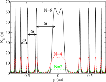
Figure 1: Comb function $K_{N}(p)$ corresponding to $N=8$ (solid), $N=4$ (dashed) and $N=2$ (dotted-dashed) IR cycles, for both one or two attosecond pulses per IR cycle. The IR intensity is $I=1.3\times 10^{13}$ W/cm² and the excess energy $\varepsilon_{\mathrm{f}}=0.144$ au.

Next we evaluate Eq. (8) for two atto pulses per IR cycle, $\nu=2$. Apart from pulses at $t_{n}=2n\pi/\omega$ we have a second sequence at $t_{n{+}1/2}=2(n{+}1/2)\pi/\omega=(2n{+}1)\pi/\omega$. A little thought reveals that for the first sequence $\Phi_{\mathrm{f}}(t_{n};p,\varphi)=\Phi_{\mathrm{f}}(0;p,\varphi)$, whereas for the second one $\Phi_{\mathrm{f}}(t_{n{+}1/2};p,\varphi)=\Phi_{\mathrm{f}}(0;-p,\varphi)$, see also appendix A. Collecting again all terms from Eq. (8) we can write $\psi^{\infty}_{2}(p,\varphi)$ in the form

$$\psi^{\infty}_{2}(p,\varphi)=a_{2}\sum_{n=0}^{N-1}e^{i2n\pi C}\left(e^{-iC\pi/2}\chi(p,\varphi)+e^{iC\pi/2}\chi(-p,\varphi)\right)\,.$$ (16)

Obviously, the sum over $n$ is the same geometric series as in Eq. (11). We call its absolute square the comb function,

$$\left|\sum_{n=0}^{N-1}e^{i2n\pi C}\right|^{2}=\frac{\sin^{2}(N\pi C)}{\sin^{2}(\pi C)}\equiv K_{N}(p)\,,$$ (17)

and show it for increasing $N$ in Fig. 1. From $\nu=1,2$ the general structure of the final wavefunction $\psi^{\infty}_{\nu}(p,\varphi)$ for an arbitrary number of atto pulses $\nu$ per IR cycle emerges: It factorizes in the comb amplitude which depends on the number of $N$ of IR cycles, and a complex wave packet containing $\nu$ sub-packets which are created by atto pulses during one IR cycle and therefore depend on the phase difference $\varphi$ of the IR pulse and the APT.

4 The photo-electron spectrum

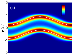
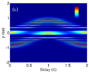
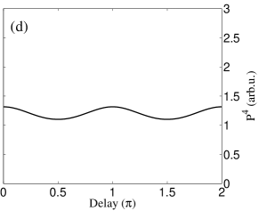
Figure 2: Results for 1 atto per IR cycle, $I=1.3\times 10^{13}$ W/cm², $\varepsilon_{\mathrm{f}}=0.144$ a.u. and $N=4$. The attosecond pulses have a width FWHM=370 as ($\sigma=$9.186). (a) $\Phi_{1}(p,\varphi)$. The white lines represent $\pm(2\varepsilon_{\mathrm{f}})^{1/2}-p_{\varphi}$. (b) Comb function $K_{4}(p)$. (c) Photo-electron spectrum, $|\Psi_{1}(p,\varphi)|^{2}$. (d) Normalized absorption probability $P^{4}(\varphi)$.

The product structure of the asymptotic wavefunction $\psi^{\infty}_{\nu}$ carries over to the photo-electron momentum distribution Eq. (9) since

$$dP_{\mathrm{\nu}}/dp=|\psi^{\infty}_{\nu}(p,\varphi)|^{2}=K_{N}(p){\cal X}_{\nu}(p,\varphi).$$ (18)

The function $K_{N}(p)$ has maxima separated in energy by the IR frequency $\omega$ which become sharper with increasing $N$, as can be seen in Fig. 1. Hence, $K_{N}(p)$ acts like a $comb$ in momentum for the photoelectron spectrum. The comb selects particular values of $p$ occurring at specific phases $\varphi$ from the electron momentum distribution ${\cal X}_{\nu}(p,\varphi)$, which builds up from the $\nu$ atto pulse wave packets within one IR period.

4.1 One atto pulse during an IR cycle

For $\nu=1$, we get from Eq. (13)

$${\cal X}_{1}(p,\varphi)=|\chi(p,\varphi)|^{2}=\exp\left\{-\frac{[(p+p_{\varphi})^{2}/2-\varepsilon_{\mathrm{f}}]^{2}}{\sigma_{\mathrm{\varepsilon}}^{2}(p)}\right\},$$ (19)

The electron distribution ${\cal X}_{1}$ shown in Fig. 2a has two branches centered about $p_{\pm}=\pm\sqrt{2\varepsilon_{\mathrm{f}}}-p_{\varphi}$. Each of them traces the streaking momentum $p_{\varphi}$ (Eq. (14) and white lines in the figure) which is imprinted when the attosecond pulse excites the electron with a phase delay $\varphi$. The width $\sigma_{\mathrm{\varepsilon}}$ of the branches has maxima at $\varphi=\frac{1}{2}\pi,\frac{3}{2}\pi$ and minima at $\varphi=0,\pi$. The multiplication of ${\cal X}_{1}$ (Fig. 2a) with the comb $K_{4}(p)$ (Fig. 2b) gives the photo-electron momentum distribution shown in Fig. 2c. One clearly sees a preference of momenta and phase delays. The modulation in phase delays survives upon integration over $p$ in the total absorption probability $P^{N_{\mathrm{atto}}}(\varphi)$ shown in Fig. 2d, with maxima at $\varphi=0,\pi$.

4.2 Two atto pulses during an IR cycle

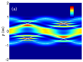
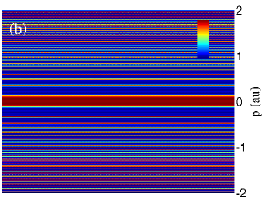
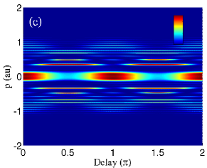
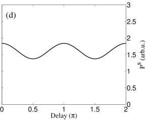
Figure 3: Same as in Fig. 2 $(N=4)$, but for $\nu=2$ atto pulses per IR period $(N_{\mathrm{atto}}=8)$. The white lines in (a) correspond to different branches in the wave packet ${\cal X}$, see text.

While the comb function remains the same, we have now a more complicated single cycle momentum distribution composed of two wave packets during each IR cycle,

$${\cal X}_{2}(p,\varphi)=\left|e^{-iC\pi/2}\chi(p,\varphi)+e^{iC\pi/2}\chi(-p,\varphi)\right|^{2}\,.$$ (20)

The basic structure with two branches for each wave packet $\chi$ is the same as for $\nu=1$, resulting in a total of four branches at $p_{\pm}^{+}=\pm\sqrt{2\varepsilon_{\mathrm{f}}}-p_{\varphi}$ and $p_{\pm}^{-}=\pm\sqrt{2\varepsilon_{\mathrm{f}}}+p_{\varphi}$, indicated as white lines (solid and dashed, respectively) in Fig. 3a. In addition, the wave packets interfere leading to a rich pattern in ${\cal X}_{2}$, as can be seen in Fig. 3a. However, again the comb $K_{4}(p)$, cf. Fig. 3b, selects specific momenta and phases for the photo-electron momentum distribution Fig. 3c, which produces a modulation in the total absorption probability (Fig. 3d) similarly as for $\nu=1$, with maxima at $\varphi=0,\pi$. Note, that for both $\nu=1$ and $\nu=2$ the number of maxima in the absorption probability $P_{\mathrm{\nu}}(\varphi)$ is the same.

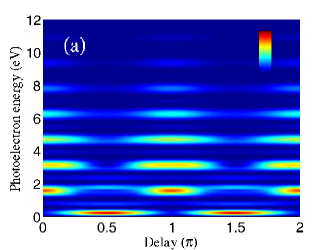
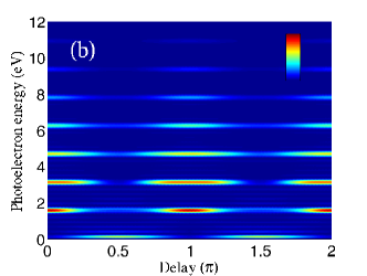
Figure 4: Photo-electron energy spectra for an intensity $I=1.3\times 10^{13}$ W/cm², excess energy $\varepsilon_{\mathrm{f}}=-0.028$, $\nu=2$ and $N$=3 (a) and $N$=6 (b) IR cycles.

The effect of an increasing number $N$ of IR cycles in the comb $K_{N}(p)$ on the photo-electron spectrum is shown in Fig. 4 for the same intensity as before, but for an excess energy $\varepsilon_{\mathrm{f}}=-0.028$ and $\nu=2$. The narrower lines for larger $N$ (Fig. 4b as compared to Fig. 4a) is due to the sharper comb for larger $N$.

For the cases shown in Figs. 2, 3 and 4 the maxima appear at $\varphi=0,\pi$ and the absorption probabilities have similar shapes. This is not always the case. Rather, the position of the maxima and the contrast between maxima and minima depend on the particular comb $K_{N}$ and therefore on $N$, $U_{\mathrm{p}}$ and $\varepsilon_{\mathrm{f}}$, as well as on the details of the branches in the wave packet ${\cal X}_{\nu}$. This will be discussed in the next section.

5 Position of the maxima and minima in the absorption probability

We have seen how the oscillations in the absorption probability arise from the interplay between the comb function $K_{N}(p)$ and the momentum distribution ${\cal X}_{\nu}$ of a multi-component wave packet. Both depend in a complex manner on the parameters of the laser fields and the groundstate energy of the atom. Hence the question arises if one can predict analytically for a given IR field intensity, where the maxima in $P_{\mathrm{\nu}}(\varphi)$ appear as a function of phase delay for different VUV photon energies $\Omega$ of the APT.

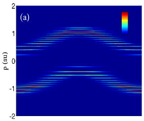
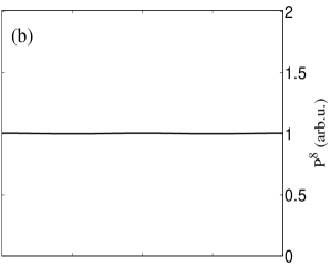
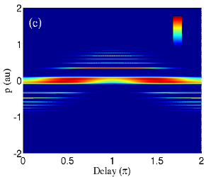
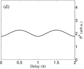
Figure 5: Photo-electron momentum distribution (left) and corresponding absorption probability (right) for $\nu=1$, $I=1.3\times 10^{13}$ W/cm², $N=8$ and $\varepsilon_{\mathrm{f}}=0.28$ a.u. (upper panels) and $\varepsilon_{\mathrm{f}}=-0.028$ a.u. (lower panels).

From the structure of the comb as discussed in Sect. 4 one can directly conclude that the oscillations in $P_{\mathrm{\nu}}(\varphi)$ will disappear for increasing $\varepsilon_{\mathrm{f}}=\varepsilon_{\mathrm{i}}+\Omega$, as illustrated in Fig. 5a. For large excess energy $\varepsilon_{\mathrm{f}}$ the branches of ${\cal X}$ are centered about high absolute momentum values $|\pm(2\varepsilon_{\mathrm{f}})^{1/2}\pm p_{\varphi}|$, where the comb is dense. Hence, the comb traces ${\cal X}(p,\varphi)$ homogeneously for all $\varphi$ and the absorption probability hardly depends on $\varphi$ (Fig. 5b). The physical meaning of this is that when the electronic wave packet triggered by an atto pulse leaves the nucleus with a high kinetic energy, the overlap with the EWPs released by subsequent atto pulses vanishes, which diminishes the intereference among the wave packets.

A more systematic analysis of the position of the maxima and minima in the absorption probability can be carried out analytically using symmetry properties of $P_{\nu}$ and eventually a stationary phase approximation with respect to $p$. The condition for extrema is $dP_{\nu}/d\varphi=0$, which can be written for the case of $\nu=1$ as

$$\frac{dP_{1}}{d\varphi}=\int\,dpK_{N}(p){\cal X}^{\prime}_{1}(p,\varphi)=0,$$ (21)

where ${\cal X}^{\prime}_{1}(p,\varphi)=\partial{\cal X}_{1}(p,\varphi)/\partial\varphi$, which is proportional to $x_{\varphi}$. Therefore, the absorption probability has extrema for $x_{\varphi}=0$. The symmetry of the functions under the integral reveals another set of maxima: the comb $K_{N}(p)$ is even in $p$, and for $p_{\varphi}=0$, the function ${\cal X}^{\prime}_{1}$ is odd in $p$. Hence, the integral in Eq. (21) is zero and there are also extrema for $p_{\varphi}=0$. To summarize, Eq. (21) is fulfilled for every $\varphi=n\pi/2$.

To distinguish between maxima and minima we need the sign of the second derivative, ${\cal X}_{1}^{\prime\prime}$. To keep the derivation simple we will make now use of the stationary phase approximation, which is applicable since the comb $K_{N}(p)$ is a highly oscillatory function which depends only on $p^{2}$. Therefore, its global stationary phase point is $p=0$, which is also obvious from Fig. 1, and we get for Eq. (21)

$$\frac{dP_{1}}{d\varphi}\sim K_{N}(0){\cal X}^{\prime}_{1}(0,\varphi),$$ (22)

where

$${\cal X}^{\prime}_{1}(0,\varphi)={\cal X}_{1}(0,\varphi)\;\frac{d}{d\varphi}\left[-\left(p_{\varphi}^{2}/2-\varepsilon_{\mathrm{f}}\right)^{2}\Big{/}\sigma_{\mathrm{\varepsilon}}^{2}(0)\right].$$ (23)

It can be easily shown that this function is zero for $x_{\varphi}=0$ or $p_{\varphi}=0$ as before, and has additional zeros at $p_{\varphi}^{2}=2\varepsilon_{\mathrm{f}}$. For the determination of maxima and minima we are only interested in the sign of the second derivative, which can be expressed for the three groups of extrema as

$$\mathrm{sgn}\left[\left.{\cal X}_{1}^{\prime\prime}(0,\varphi)\right|_{\varphi=n\pi}\right] = \mathrm{sgn}\left[g(2U_{\mathrm{p}}-\varepsilon_{\mathrm{f}})\right]$$ (24)

$$\mathrm{sgn}\left[\left.{\cal X}_{1}^{\prime\prime}(0,\varphi)\right|_{\varphi=(n{+}1/2)\pi}\right] = \mathrm{sgn}\left[g(\varepsilon_{\mathrm{f}})\right]$$ (25)

$$\left.{\cal X}_{1}^{\prime\prime}(0,\varphi)\right|_{p_{\varphi}^{2}=2\varepsilon_{\mathrm{f}}}=-8\frac{\varepsilon_{\mathrm{f}}(2U_{\mathrm{p}}{-}\varepsilon_{\mathrm{f}})}{\sigma_{\mathrm{\varepsilon}}^{2}}<0\qquad 0\leq\varepsilon_{\mathrm{f}}\leq 2U_{\mathrm{p}}$$ (26)

with $g(x)=x(1+4\sigma^{4}\omega^{2}U_{\mathrm{p}}x)8\sigma^{2}U_{\mathrm{p}}{\cal X}_{1}(0,\varphi)$. This leaves a clear structure of maxima and minima for $\varepsilon_{\mathrm{f}}<0$ and $\varepsilon_{\mathrm{f}}>2U_{\mathrm{p}}$ as summarized in Table 1. For $0<\varepsilon_{\mathrm{f}}<2U_{\mathrm{p}}$, all four extrema within $2\pi$ are minima, making the approximation not very trust worthy. Indeed, as will be demonstrated later, chaotic dynamics dominates this energy region rendering approximations problematic. In Fig. 6a one can see this structure of maxima and minima in $\varphi$ additionally modulated in $\varepsilon_{\mathrm{f}}$, where the distance between the maxima is $\omega$. The latter is a consequence of the effect of the comb function $K_{N}(0)$, which has maxima at $C_{0}\pi=n\pi$ (with $C_{0}=C|_{p=0}$), which means maxima at energies $\varepsilon_{\mathrm{f}}=U_{\mathrm{p}}\pm n\omega$.

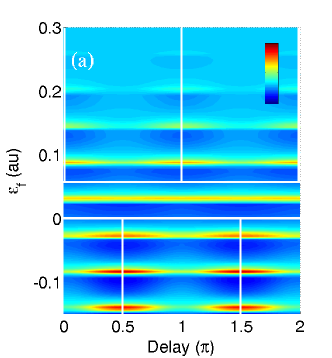
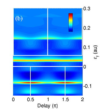
Figure 6: Absorption probability as a function of $\varphi$, for 1 (a) and 2 (b) atto pulses per IR cycle, for $I=1.3\times 10^{13}$ W/cm² and $N$=8. Vertical white lines: position of the maxima at $\varepsilon_{\mathrm{f}}$ in the two regions $\varepsilon_{\mathrm{f}}<0$ and $\varepsilon_{\mathrm{f}}>2U_{\mathrm{p}}$, as predicted with the SPA: at $\varphi$=$\pi/2$ and $3\pi/2$ in the first case and at 0, $\pi$ and $2\pi$ in the second. The horizontal white lines differentiate these two regions.

energy	$\varphi=n\pi$	$\varphi=(n{+}1/2)\pi$
$\varepsilon_{\mathrm{f}}>2U_{\mathrm{p}}$	maximum	minimum
$\varepsilon_{\mathrm{f}}<0$	minimum	maximum

Table 1: Position of the maxima and minima in $\varphi$ for different energy ranges $\varepsilon_{\mathrm{f}}$.

Moving on to the case $\nu=2$ we investigate $P_{2}(\varphi)$ taking ${\cal X}_{2}$ from Eq. (20), and for the sake of simplicity we will use the stationary phase approximation from the beginning. This function has the same stationary phase point $p=0$ as before. Then we can write

$${\cal X}_{2}(0,\varphi)=4\cos(C_{0}\pi/2){\cal X}_{1}(0,\varphi)\,.$$ (27)

From Eq. (27) it is immediately clear that the $\nu=2$ case has the same structure of maxima and minima with respect to the phase delay $\varphi$ (see table 1) as the $\nu=1$ case. The only difference is the modulation in $\varepsilon_{\mathrm{f}}$: The additional factor $\cos[C_{0}\pi/2]$ has maxima only at even multiples of the IR frequency $\varepsilon_{\mathrm{f}}=U_{\mathrm{p}}\pm 2n\omega$, while it has zeros at odd multiples of $\omega$. Consequently, the distance between the peaks for $\nu=2$ on the $\varepsilon_{\mathrm{f}}$ axis is given by $2\omega$ instead of $\omega$ as for $\nu=1$, which can be seen in Fig. 6.

6 Comparison with experimental results and exact quantum calculations

The interesting dependence of the absorption probability on the phase delay $\varphi$ was first reported experimentally and shown to be in agreement with a full numerical quantum calculation by Johnsson et al. [8]. In the meantime it has been confirmed by other experiments [13]. Instead of increasing the VUV photon energy (to vary $\varepsilon_{\mathrm{f}}=\varepsilon_{\mathrm{i}}+\Omega$), the ionization potential $-\varepsilon_{\mathrm{i}}$ was varied in the first experiment [8] by using He and Ar atoms as targets for the combined IR + APT field, the latter with two atto pulses per IR cycle and a central energy of $\Omega$=23 eV. This energy is enough to ionize an electron from Ar, but not from He (see inset in Fig. 7). Strong oscillations in the ionization probability of He as a function of $\varphi$ were found with maxima at $\varphi=(n+1/2)\pi$ and no oscillations were detected for Ar.

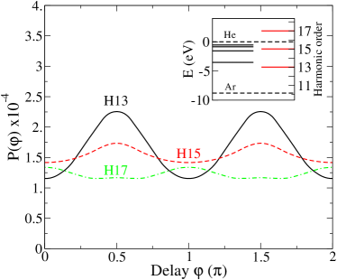
Figure 7: Quantum calculation for the absorption probability for an IR with $\lambda$=796 nm, $I=1.3\times 10^{13}$ W/cm² and an APT with FWHM=5 fs, and three different central energies: the 13^th harmonic of the IR field (full line), the 15^th (dashed line) and the 17^th (dashed-dotted line). The energy levels of the He atom are shown in the inset (full black lines), together with the ionization threshold of He and Ar (dashed lines). The energies for the 13^th, 15^th and 17^th are also shown (red lines at the right).

These results are in qualitative agreement with our analytical predictions, as shown in Fig. 6b. For $\varepsilon_{\mathrm{f}}<0$ (as in He with $\Omega$=23 eV), we expect maxima at $\varphi=(n+1/2)\pi$ , while for energies well above threshold as in Ar, we expect a flat absorption probability. To double check the transition from the positions of the maxima from $(n{+}1/2)\pi$ to $n\pi$ going from $\varepsilon_{\mathrm{f}}<0$ to positive $\varepsilon_{\mathrm{f}}$, we have performed full numerical calculations. We use a three-dimensional one-electron model for the He atom, and a classical electric field, with $\omega=0.0572$, $I=1.3\times 10^{13}$ W/cm² for the IR, and $I=10^{11}$ W/cm² for the APT. Results are shown in Fig. 7 for three different APTs, centered at the harmonics 13^th, 15^th and 17^th, respectively. One sees indeed that the contrast of the maxima gets smaller for increasing but still negative $\varepsilon_{\mathrm{f}}$, as it is the case going from the 13^th to the 15^th harmonic while for positive $\varepsilon_{\mathrm{f}}$ (17^th harmonic), there appear maxima at $\varphi=0,\pi$.

Figure 8: Contrast (Eq. (28)) of maxima and minima in the absorption probability for $\nu=2$ atto pulses per IR period. Straight line: analytical approach. Dashed line: TDSE calculations, for an APT with central energy from the 13^th to 17^th harmonics. The energies for the 13^th, 15^th and 17^th harmonics are pointed out. The conditions are $N=4$ ($N_{\mathrm{atto}}=8$), $I=1.3\times 10^{13}$ W/cm² and $\lambda=$796 nm. The ionization threshold is marked by a vertical line.

Hence, the simple man’s approach presented here provides in general a very good understanding and interpretation of the effect a combined APT and IR field has on the ionization of atoms. Only for energies $\varepsilon_{\mathrm{f}}$ very close to the ionization threshold, $|\varepsilon_{\mathrm{f}}|\approx U_{\mathrm{p}}$ the simple man’s approach is too drastic for reliable results. In this energy range, the oscillatory absorption probability depends sensitively on details of the electronic wave packet whose dynamics is highly chaotic. This is demonstrated in Fig. 8 for a sensitive observable, the contrast between maxima (at $\varphi_{\mathrm{max}}$) and minima (at $\varphi_{\mathrm{min}}$) for different photon energies,

$$A=\frac{P(\varphi_{\mathrm{max}})-P(\varphi_{\mathrm{min}})}{P(\varphi_{\mathrm{max}})+P(\varphi_{\mathrm{min}})}\,.$$ (28)

One may question if such details of the chaotic behavior are helpful to understand the dynamics. Future work will show if more robust observables, such as correlation functions with characteristic correlation lengths and similar quantities are more suitable to characterize electron dynamics under the illumination of APTs and IR fields.

7 Conclusions and outlook

We have presented a minimal analytical approach to understand the behavior of electron wave packets generated by an attosecond pulse train (APT) in the presence of a strong IR field in the framework of the simple man’s approach in strong field physics, with special emphasis in the phase delay between the APT and IR pulses. In this approximation the photo absorption probability can be written as a product of a frequency comb function, resulting from the periodic nature of the pulses with the IR frequency, and the probability density of an electronic wave packet whose number of components is given by the number of attosecond pulses within on IR period. Only the latter depends on the phase delay between APT and IR field, while the former acts like an electron momentum filter. The minimal approach provides insight into the formation of oscillations in the photo-absorption as a function of phase delay, on the frequency of these oscillations and the general trend of the phase delay as a function of excess (or photon) energy. The minimal approach fails for excess energies comparable with the ponderomotive potential, where the chaotic nature of the electron dynamics renders results very sensitive to approximations.

Appendix A Taylor expansion of the phase

The functions $F^{(k)}_{n}=d^{k}\phi_{n}(t)/dt^{k}\Big{|}_{t=t_{n}}$ needed in Eq. (8) are

$$F^{(0)}_{n}=i\int^{t_{n}}\frac{(p+A(\tau))^{2}}{2}\,d\tau-i\varepsilon_{\mathrm{f}}t_{n}\,,$$ (29)

$$F^{(1)}_{n}=i\frac{(p+A(t_{n}))^{2}}{2}-i\varepsilon_{\mathrm{f}}\,,$$ (30)

$$F^{(2)}_{n}=i(p+A(t_{n}))A^{\prime}(t_{n})-\frac{1}{\sigma^{2}}\,.$$ (31)

Their explicit values for $t_{n}=2\pi n/\omega$ are

$$F^{(0)}_{n}=F_{0}+i2n\pi C+ipx_{\mathrm{\varphi}}\,,$$ (32)

$$F^{(1)}_{n}=i\frac{(p+p_{\mathrm{\varphi}})^{2}}{2}-i\varepsilon_{\mathrm{f}}\,,$$ (33)

$$F^{(2)}_{n}=-i(p+p_{\mathrm{\varphi}})\omega^{2}x_{\mathrm{\varphi}}-\frac{1}{\sigma^{2}}\,,$$ (34)

where $C$, $x_{\varphi}$ and $p_{\varphi}$ are defined in Eq. (12) and Eq. (14), respectively. $F_{0}$ is a phase that does not contribute to $|\psi^{\infty}_{\nu}(p,\varphi)|^{2}$ (Eq. (9)).

For two atto pulses per IR cycle ($\nu=2$) we have in additional set of quantities $F^{(k)}_{n{+}1/2}$. They differ from the values of the $F^{(k)}_{n}$ in Eqs. (32) – (34) only in two respects: The term $i2n\pi C$ in $F^{(0)}_{n}$ has to be modified to $i(2n{+}1)\pi C$ and in all quantities $p$ has to be replaced by $-p$, which follows from of the Volkov propagator (6).

References

References

- [1] Paul P. M., Toma E. S., Breger P., Mullot G., Augé F., Balcou P., Muller H. G. and Agostini P. 2001 Science 292 1689
- [2] Johnsson P. et al. 2005 Phys. Rev. Lett. 95 013001
- [3] Guyétand O. et al. 2005 J. Phys. B 39 3983
- [4] Figueira de Morisson Faria C., Salières P., Villain P. and Lewenstein M. 2006 Phys. Rev. A 74 053416
- [5] Yudin G. L., Patchkovskii S. and Bandrauk A. D. 2008 J. Phys. B 41 045602
- [6] Van der Hart H. W., Lysaght M. A. and Burke P. G. 2008 Phys. Rev. A 77 065401
- [7] Remetter T. et al. 2006 Nature Phys. 2 323 (2006)
- [8] Johnsson P., Mauritsson J., Remetter T., L’Huillier A. and Schafer K. J. 2007 Phys. Rev. Lett. 99 233001
- [9] Lewenstein M., Balcou P., Ivanov M. Y., L’Huiller A. and Corkum P. B. 1994 Phys. Rev. A 49 2117
- [10] Smirnova O., Spanner M. and Ivanov M. 2008 Phys. Rev. A 77 033407
- [11] van de Sand G. and Rost J. M. 2000 Phys. Rev. A 62 053403
- [12] Rivière P., Ruiz C. and Rost J. M. 2008 Phys. Rev. A 77 033421
- [13] Cocke C. L., private communication and presentation at ICOMP XX, Heidelberg (2008).
- [14] Quéré F., Mairesse Y. and Itatani J. 2005 J. Mod. Opt. 52 339
- [15] Mauritsson J., Johnsson P., Gustafsson E., L’Huillier A., Shafer K. J. and Gaarde M. B. 2006 Phys. Rev. Lett. 97 013001