Stability analysis of confined V-flames. I. Analytical treatment
of the high-velocity limit

Abstract

The problem of linear stability of confined V-flames with arbitrary gas expansion is addressed. Using the on-shell description of flame dynamics, a general equation governing propagation of disturbances of an anchored flame is obtained. This equation is solved analytically for V-flames in high-velocity channel streams. It is demonstrated that dynamics of flame disturbances in this case is controlled by the memory effects associated with vorticity generated by the curved front. The perturbation growth rate spectrum is determined, and explicit analytic expressions for the eigenfunctions are given. It is found that the piecewise linear V-structure is unstable for all values of the gas expansion coefficient.

I Introduction

Among the various types of premixed flame propagation problems, anchored flames hold a special place. On the one hand, such flames are relatively easy to realize experimentally; on the other, they look simple enough for theoretical investigation, because they admit several important simplifications. For instance, open flames anchored by means of a thin rod are often observed to have rectilinear wings (unconfined V-flames). Homogeneity of the upstream flow, adopted usually as the natural approximation compatible with this piecewise linear flame-front structure, often conveys the impression that the problem is easily solvable analytically. It thus represents an excellent laboratory for testing our understanding of premixed flame dynamics.

Despite these promising circumstances there is an apparent lack of theoretical results on V-flame properties. The reason is that these flames are not as simple as they seem. A closer inspection of the flow structure of the idealized V-configuration reveals that this pattern is singular: the pressure field turns out to diverge logarithmically near the tip of the flame-front (and also at infinity along the front, in the case of unconfined V-flames). This is a sign of incompleteness of the idealized picture, which means that the system anchoring the flame must be explicitly included into consideration. This essential complication necessitates the introduction of a specific inner scale in the problem (in addition to the cutoff wavelength and the channel width), thereby raising the question as to the influence of this new scale on the whole basic pattern. The initial problem is thus naturally divided into two parts: 1) modeling of the anchoring system; this primarily is a stationary analysis, aimed at inferring properties of the system needed to generate a presumed flame pattern, and 2) investigation of the flame dynamics, which first and foremost is a stability analysis of the anchored flame; an important issue in this analysis is its model-dependence, i.e., the extent to which its results depend on particularities of the anchoring system.

The purpose of the present paper is to carry out an analysis of the above-mentioned issues, in the case of a confined V-flame anchored in a high-velocity gas stream. It will be shown that the problem admits a full theoretical investigation in this important particular case, and that its results are model-independent in the above sense. It should be mentioned that in contrast to unconfined anchored flames, flames anchored in channels do not exhibit an acute linear structure, although the piecewise linear front with a uniform upstream flow is still a solution of the governing equations. Experiments show that deviations from linearity occur not only in the small regions near the anchor and the channel walls, but all along the front (Scurlock, 1948; pro, 1949; Zel’dovich et al., 1985). This suggests that the simplest configuration is possibly unstable in the confined case. The results of our work fully confirm this conjecture.

In our investigation, we use the on-shell description of flames developed in Refs. (Kazakov, 2005a, b; El-Rabii et al., 2008; Joulin et al., 2008). The integro-differential equations derived therein provide a non-perturbative description of spontaneous flame dynamics in the most general form, i.e., they apply to flames with arbitrary gas expansion and arbitrary jump conditions across the flame front. The main advantage of using these equations is that they are closed, in the sense that they involve only quantities defined at the flame front. This allows one to avoid explicit solving of the flow equations in the bulk, which is the stumbling block of conventional analysis. This approach will be shown to be extendable to the case of anchored flames in a simple and natural way.

The paper is organized as follows. Section II serves to set up the general framework of the on-shell flame description. In Sec. II.1, we formulate the problem and recall the main results of Refs. (Kazakov, 2005a, b; El-Rabii et al., 2008; Joulin et al., 2008). Extension of these results to the case of anchored flames is described in Sec. II.2. An analysis of the anchoring system impact on the flame structure, carried out in Sec. II.3, is used in Sec. II.4.1 to identify boundary conditions for the linearized equation describing the propagation of disturbances. This equation is derived, in a form suitable for the subsequent analysis, in Sec. II.4, then solved in Sec. III. An important step here is the evaluation of rotational contribution, presented in Sec. III.1. The resulting equation is analyzed in the high-velocity limit in Sec. III.2, which allows considerable simplifications. In particular, an asymptotic expansion of the main integral operator $\mathcal{H}$ is constructed in Sec. III.2.1. Finally, analytic solutions of the linearized problem are found in Sec. III.3, and studied in detail in Sec. III.4. Section IV contains concluding remarks and prospects for future work. The paper has two appendices, one of which contains a consistency check for the calculations performed, and the other describes in detail transition to the case of vanishingly small anchor dimensions within the large-slope expansion.

II Preliminaries

II.1 Spontaneous flame dynamics on-shell

Consider a 2D-flame propagating in a channel of constant width $b,$ filled with an initially quiescent uniform ideal gas. Let the Cartesian coordinates $(x,y)$ be chosen so that the channel walls are at $x=0,b,$ and $y=-\infty$ is in the fresh gas. These coordinates will be measured in units of the channel width, while fluid velocity, $\bm{v}=(w,u),$ in units of the velocity of a plane flame front relative to the fresh gas, $U_{f}.$ Finally, the fluid density will be normalized by the fresh gas density, $\theta>1$ denoting its ratio to that of burnt gas. We assume that the flame pattern is continued to the whole $x$-axis in the usual way using the ideal boundary conditions at the channel walls:

$$f^{\prime}=0,\quad w=0\quad{\rm for}\quad x=0,b\,.$$ (1)

Then the on-shell value, $(w_{-},u_{-})$, of fresh-gas velocity (i.e., its value at the flame front considered as a gasdynamic discontinuity), and the flame front position, $f(x,t),$ satisfy the following complex integro-differential equation (El-Rabii et al., 2008; Joulin et al., 2008)

$$2\left(\omega_{-}\right)^{\prime}+\left(1+i\hat{\mathcal{H}}\right)\left\{[\omega]-\frac{i}{4}\int\limits_{-\infty}^{+\infty}d\tilde{x}(i\partial_{y}-\partial_{x})\int\limits_{\tau_{-}}^{\tau_{+}}d\tau M(\tilde{x},t-\tau)\right\}^{\prime}=0\,,$$ (2)

where $\omega=u+iw$ is the complex gas velocity, $[\omega]$ its jump across the flame front, $\partial_{x}\equiv\partial/\partial x,$ $\partial_{y}\equiv\partial/\partial y,$ and the prime denotes differentiation with respect to $x$ (in the last term on the left, the argument $y$ is understood to be set equal to $f(x,t)$ after partial spatial differentiation, but before the $x$-differentiation denoted by the prime; we recall that the improper $\tilde{x}$-integral in this term is understood as an analytic continuation of the corresponding regularized expression, see Ref. (Joulin et al., 2008) for details). The memory kernel $M$ has the form $M(\tilde{x},t)\equiv N(\tilde{x},t)\bar{v}^{n}_{+}(\tilde{x},t)\sigma_{+}(\tilde{x},t),$ where $N=\sqrt{1+\left(f^{\prime}\right)^{2}}\,,$ $\bar{v}^{n}_{+}=\bar{v}_{i+}n_{i}$ is the normal burnt gas velocity relative to the flame front, $n_{i}$ denoting the unit vector normal to the front ($\bm{n}$ points towards the burnt gas), and $\sigma_{+}$ is the on-shell value of vorticity produced by the curved front. The memory kernel is integrated over any path in the complex time-plane, connecting the points

$$\tau_{\pm}=\frac{r}{\bar{v}_{+}}\left(\Omega\pm i\sqrt{1-\Omega^{2}}\right)\,,\quad\Omega\equiv\frac{(\bm{r}\cdot\bar{\bm{v}}_{+})}{r\bar{v}_{+}}\,,$$

where

$$\bar{\bm{v}}_{+}=(w_{+},\bar{u}_{+})\,,\quad\bar{u}_{+}(x,t)\equiv u_{+}(x,t)-\frac{\partial f(x,t)}{\partial t}$$

is the on-shell burnt gas velocity relative to the front, and $\bm{r}$ is the radius-vector drawn from the point $(\tilde{x},f(\tilde{x},t))$ at the front to the observation point $(x,y).$ Finally, the action of the operator $\hat{\mathcal{H}}$ on an arbitrary function $a(x)$ is defined by

$$\left(\hat{\mathcal{H}}a\right)(x)=\frac{1+if^{\prime}(x,t)}{\pi}~{}\fint\limits_{-\infty}^{+\infty}d\tilde{x}~{}\frac{a(\tilde{x})}{\tilde{x}-x+i[f(\tilde{x},t)-f(x,t)]}\,,$$ (3)

where the slash denotes the principal value of the integral. For a $2b$-periodic function $a(x)$ [i.e., $a(x+2b)=a(x)$], summing explicitly the integrand with the help of the formula

$$\sum\limits_{k=-\infty}^{+\infty}\frac{1}{2bk+z}=\frac{\pi}{2b}\cot\left(\frac{\pi z}{2b}\right),$$

the right hand side of (3) can be rewritten as an integral over the channel width

$$\left(\hat{\mathcal{H}}a\right)(x)=\frac{1+if^{\prime}(x,t)}{2b}~{}\fint\limits_{-b}^{+b}d\tilde{x}~{}a(\tilde{x})\cot\left\{\frac{\pi}{2b}(\tilde{x}-x+i[f(\tilde{x},t)-f(x,t)])\right\}\,.$$ (4)

We recall also that the value of vorticity at the front and the normal velocity of the burnt gas, entering the function $M(\tilde{x},t-\tau),$ as well as the velocity jumps at the front, are all known functionals of on-shell fresh gas velocity (Matalon and Matkowsky, 1982; Pelce and Clavin, 1982). For zero-thickness flame fronts one has

$$\bar{v}^{n}_{+} = \theta\,,\quad[u]=\frac{\theta-1}{N}\ ,\quad[w]=-f^{\prime}\frac{\theta-1}{N}\,,$$ (5)

$$\sigma_{+} = -\frac{\theta-1}{\theta N}\left[\frac{Dw_{-}}{Dt}+f^{\prime}\frac{Du_{-}}{Dt}+\frac{1}{N}\frac{Df^{\prime}}{Dt}\right]\,,$$ (6)

where

$$\frac{D}{Dt}\equiv\frac{\partial}{\partial t}+\left(w_{-}+\frac{f^{\prime}}{N}\right)\frac{\partial}{\partial x}\,.$$

Together with the evolution equation

$$(\bar{\bm{v}}_{-}\cdot\bm{n})=1\,,$$ (7)

the complex Eq. (2) constitutes a closed system of three equations for the three functions $w_{-}(x,t),$ $u_{-}(x,t)$ and $f(x,t).$

II.2 On-shell description of anchored flames

As derived, Eq. (2) describes only spontaneous flame evolutions. However, the anchoring system is not difficult to incorporate into the framework of the on-shell description. This can be done as follows. Consider the simplest and most commonly used in practice type of the anchoring system – a metal rod placed somewhere within the channel. From the mathematical point of view, the presence of the rod can be described as a singularity of the complex velocity, $\omega=u+iw,$ considered as an analytical function of the complex variable $z=x+iy.$ Namely, suppose that the original field, $\omega_{0}(z),$ is superimposed with the complex velocity, $\omega^{d}(z),$ describing a dipole located at the point $(x_{0},y_{0})$:

$$\omega_{0}(z)+\frac{d}{(z-z_{0})^{2}}\equiv\omega(z)\,,$$ (8)

where $z_{0}=x_{0}+iy_{0},$ and $d=d_{1}+id_{2}$ is a complex constant determining strength of the dipole as well as its orientation. For sufficiently small $|d|,$ perturbation of the main flow is noticeable only in a small vicinity of the dipole. Since $\omega_{0}(z)$ is analytical at $z=z_{0},$ one has

$$\omega_{0}(z)=\omega_{0}(z_{0})+O(|z-z_{0}|),$$

and hence, the complex velocity near the dipole can be written approximately as

$$\omega(z)\approx\omega_{0}(z_{0})+\frac{d}{(z-z_{0})^{2}}\,.$$ (9)

The form of the stream lines is given by

$${\rm Re}\left\{\omega_{0}(z_{0})(z-z_{0})-\frac{d}{z-z_{0}}\right\}={\rm const}\,,$$

or

$$u_{0}(x-x_{0})-w_{0}(y-y_{0})-\frac{d_{1}(x-x_{0})+d_{2}(y-y_{0})}{(x-x_{0})^{2}+(y-y_{0})^{2}}={\rm const}\,,$$

where $u_{0},w_{0}$ are the real and imaginary parts of $\omega_{0}(z_{0}).$ It is seen that if we choose $d_{1}=u_{0}R^{2},$ $d_{2}=-w_{0}R^{2},$ with $R$ arbitrary real, then the stream-line family contains a circle of radius $R,$ centered at the point $(x_{0},y_{0}).$ Thus, adding the term $\omega^{d}(z)=\omega^{*}_{0}(z_{0})R^{2}/(z-z_{0})^{2}$ to the velocity field $\omega_{0}(z)$ describes perturbation of the given flow by a cylindrical rod of radius $R,$ centered at $z_{0}.$ To take into account non-uniformity of the main flow near the rod, and to describe more general rod profiles, it will be necessary to superpose several dipoles located within the rod area, and to include higher-order multipoles into consideration.

To obtain generalization of Eq. (2) to the case of anchored flames, we recall that this equation is a consequence of the following relations:

$$\left(1-i\hat{\mathcal{H}}\right)\left(\omega_{-}\right)^{\prime}=0\,,$$ (10)

$$\left(1+i\hat{\mathcal{H}}\right)\left(\omega^{p}_{+}\right)^{\prime}=0\,,$$ (11)

$$\omega^{v}_{+}=\frac{i}{4}\int\limits_{-\infty}^{+\infty}d\tilde{x}(i\partial_{y}-\partial_{x})\int\limits_{\tau_{-}}^{\tau_{+}}d\tau M(\tilde{x},t-\tau)$$ (12)

$$\omega^{p}_{+}=-\omega^{v}_{+}+\omega_{-}+[\omega]\,,$$ (13)

where $[\omega]$ denotes the jump of the complex velocity across the flame front, $[\omega]=\omega(x,f(x,t)+0)-\omega(x,f(x,t)-0).$ Equations (10), (11) express analyticity and boundedness of the complex velocity upstream, and its potential component downstream (Kazakov, 2005a, b), Eq. (12) is the on-shell expression of the rotational component (Joulin et al., 2008), while Eq. (13) is an obvious identity. As we have just seen, the presence of the rod violates analyticity of the complex velocity, so that either of Eqs. (10), (11) is no longer valid, depending on whether the rod is placed up- or downstream. In the former case, Eq. (10) is satisfied by $\omega_{0}(z)=\omega(z)-\omega^{d}(z),$ because it is analytical upstream and bounded. On the other hand, since $\omega^{d}(z)$ does not have singularities downstream and is bounded there, it satisfies Eq. (11). Thus,

$$\left(1-i\hat{\mathcal{H}}\right)\left(\omega_{-}-\omega^{d}_{-}\right)^{\prime}=0\,,$$

$$\left(1+i\hat{\mathcal{H}}\right)\left(\omega^{d}_{+}\right)^{\prime}=0\,.$$

Since $\omega^{d}_{-}=\omega^{d}_{+},$ we see that Eq. (10) is replaced in this case by

$$\left(1-i\hat{\mathcal{H}}\right)\left(\omega_{-}\right)^{\prime}=2\left(\omega^{d}_{-}\right)^{\prime}\,.$$ (14)

Accordingly, acting on Eq. (13) by the operator $(1+i\hat{\mathcal{H}}),$ we obtain the following equation

$$2\left(\omega_{-}\right)^{\prime}+\left(1+i\hat{\mathcal{H}}\right)\left\{[\omega]-\frac{i}{4}\int\limits_{-\infty}^{+\infty}d\tilde{x}(i\partial_{y}-\partial_{x})\int\limits_{\tau_{-}}^{\tau_{+}}d\tau M(\tilde{x},t-\tau)\right\}^{\prime}=2\left(\omega^{d}_{-}\right)^{\prime}\,,$$ (15)

which is the sought extension of Eq. (2) to the case of anchored flames. In the case of the rod located downstream, similar considerations show that Eq. (11) must be replaced by the following

$$\left(1+i\hat{\mathcal{H}}\right)\left(\omega^{p}_{+}-\omega^{d}_{+}\right)^{\prime}=0\,,$$

$$\left(1-i\hat{\mathcal{H}}\right)\left(\omega^{d}_{+}\right)^{\prime}=0\,.$$ (16)

It is not difficult to verify that the resulting equation for $\omega_{-}$ in this case has exactly the same form (15).

II.3 Influence of anchoring system on V-flame structure

As was mentioned in introduction, the necessity of explicit inclusion of the anchoring system into consideration raises the question as to what extent this system affects global properties of V-flames. Let us now show that as long as linear dimensions of the rod are small compared to the channel width, so that the flame front can be considered piecewise linear, influence of the rod on the flame structure is local, in the sense that it is confined to a small region near the rod. We recall, first of all, that the relative value of the velocity disturbance caused by a dipole modeling the rod is proportional to $R^{2}/(x^{2}+y^{2})$ (for simplicity, the dipole is assumed to be at the origin). Hence, under the assumption $R\ll b,$ this disturbance is indeed negligible for the most part of the channel, except a small region $(x,y\sim R)$ near the rod. This simple reasoning is not yet sufficient to prove our statement, because it only demonstrates the locality of, so to speak, direct rod influence on the flow structure. In such an essentially nonlocal problem as deflagration, we also have to look for possible indirect consequences of this influence, related to the fact that the presence of the rod ultimately determines the basic flame pattern. The on-shell description is particularly convenient for this purpose, as it explicitly reveals the nonlocal structure of the governing equations.

For the rest of the paper, flames will be considered in the reference frame attached to the rod (the above-given formulation is invariant under transitions between different reference frames). Accordingly, the fresh-gas velocity at infinity will be denoted $U$:

$$u(x,y=-\infty,t)=U(>0).$$

We will assume in what follows that the anchoring system is stationary, i.e., its properties do not change with time. This means that these properties can be inferred from the steady-state V-flame structure. To this end, we note that the stationary version of Eq. (15) reads (here we are in the rest frame of the flame-front, so the over-bar in the notation of velocity is omitted)

$$2\left(\omega_{-}\right)^{\prime}+\left(1+i\hat{\mathcal{H}}\right)\left\{[\omega]^{\prime}-\frac{Nv^{n}_{+}\sigma_{+}\omega_{+}}{v^{2}_{+}}\right\}=2\left(\omega^{d}_{-}\right)^{\prime},$$ (17)

which follows directly from the fact that Eq. (2) reduces in this case to the stationary equation derived in (Kazakov, 2005a, b). In regions where the flame-front slope is constant and the upstream flow is homogeneous, the first term on the left as well as the expression in the curly brackets vanish, because velocity jumps are constant there, $\omega_{-}={\rm const},$ and vorticity is not produced. This expression is only non-zero in a vicinity of the rod where all the quantities involved vary rapidly. It is this rapid variation that is a possible source of indirect influence of the rod on the global flame structure. Indeed, for $R/b\to 0,$ both terms in the curly brackets have a $\delta$-functional character. If the $\delta$-singularity were not canceled in their sum, then upon the action of the $\mathcal{H}$-operator it would give rise to an expression which is non-zero everywhere in the channel. However, we have just seen that the right hand side of Eq. (17) vanishes outside of small region around the rod. Therefore, in order that this equation be satisfied, the $\delta$-contributions must cancel. To be more specific, let us assume that the rod is located downstream (which is normally the case in actual experiments), as shown in Fig. 1. Then, using Eqs. (10), (16), and the identity $\omega_{-}+[\omega]=\omega_{+},$ Eq. (17) can be conveniently rewritten as

$$\left(1+i\hat{\mathcal{H}}\right)\left\{\left(\omega_{+}\right)^{\prime}-\frac{Nv^{n}_{+}\sigma_{+}\omega_{+}}{v^{2}_{+}}\right\}=\left(1+i\hat{\mathcal{H}}\right)(\omega^{d}_{+})^{\prime}\,.$$ (18)

There are two types of $\delta$-like contributions on the left hand side of this equation, corresponding to the real and imaginary parts of the expression in the curly brackets. Since the real part is even under $x\to-x,$ its $x$-derivative is odd. Hence, the corresponding singularity is generally proportional to $\delta^{\prime}(x),$ and can be compensated by appropriately choosing the coefficient $d$ in the dipole term on the right hand side. Indeed, the on-shell value of a dipole $\omega^{a}(z)=a/(z-a)^{2},$ considered in the limit $a\to 0,$ possesses all characteristic properties of the $\delta$-function: $\omega_{+}(0)=1/a\to\infty,$ $\omega_{+}(x)\to 0,$ for $x\neq 0,$ and the integral $\int_{\Delta}dxa/(x+if(x)-a)^{2},$ taken over a region $\Delta\gg a$ around $x=0,$ has a finite value (because $f(x)$ is an even function).

Things are different, however, for the imaginary part which is odd in $x.$ In this case, the singularity is proportional to $\delta(x);$ for zero-thickness flames, for instance, contribution of the first term in the curly brackets to the singularity is equal to $-2i(\theta-1)s\delta(x)/\sqrt{1+s^{2}},$ where $s$ is the value of the front slope far from $x=0,$ as is seen from Eq. (5). Singularities of this kind cannot be compensated by any local field $\omega^{d}(z).$ Thus, we arrive at the conclusion that the assumption of piecewise linear front structure implies the absence of terms proportional to $\delta(x)$ on the left hand side of Eq. (18), i.e., that the contribution of the first term in the curly brackets is canceled by that of the second term. This requirement can be written in the following integral form

$$\int_{\Delta}dx\left\{\left(w_{+}\right)^{\prime}-\frac{Nv^{n}_{+}\sigma_{+}w_{+}}{v^{2}_{+}}\right\}=o(1)\quad{\rm for}\quad\Delta/b\to 0\,,$$ (19)

where $\Delta$: $R\ll\Delta\ll b$ is the length scale where “inner” solutions ($|x|\ll b$) are to be matched with the “outer” ones ($|x|\gg R$). Indeed, by virtue of Eq. (19), the contribution of the small region near the rod to the left hand side of Eq. (18) is also small outside that region, which is just the required absence of the $\delta$-terms. Equation (19) thus represents a condition that selects inner solutions compatible with the prescribed global flame structure.

II.4 Linearized equation for flame perturbations

In the present paper, we for are looking for possible genuine V-flame instabilities, which would be inherent to the V-configuration itself, and unrelated to the properties of a specific anchoring system. We thus assume, as was already mentioned, that this system is stationary, and the condition (19) is fulfilled. Then the equation for flame perturbation is obtained by linearizing Eq. (15) around the stationary solution, with the right hand side kept fixed. This linearized equation thus coincides formally with that derived in Ref. (El-Rabii et al., 2008; Joulin et al., 2008), but for our present purposes another form of this equation will be more appropriate, which avoids explicit differentiation of the memory kernel.

First of all, since the basic pattern is stationary, time-dependence of perturbations factorizes:

$$\delta f(x,t)=\tilde{f}(x)e^{\nu t}\,,\quad\delta w_{-}(x,t)=\tilde{w}(x)e^{\nu t}\,,\quad\delta u_{-}(x,t)=\tilde{u}(x)e^{\nu t}\,,$$ (20)

where $\nu$ is a complex constant to be found as part of the solution. Not to mix the imaginary unit entering $\nu$ with that appearing in Eq. (15), we will denote the former by $j$:

$$\nu=\nu_{1}+j\nu_{2},$$

where $\nu_{1,2}$ are real numbers. Accordingly, the amplitudes $\tilde{f},\tilde{w},\tilde{u}$ are to be understood complex with respect to $j$ (until Sec. III.4, $j$ will not appear in formulas explicitly; an example illustrating the use of this “double imaginary unit” formalism is given in Appendix A). Next, taking into account that the basic solution is piecewise constant, we obtain the following equation for the $x$-dependent parts of the perturbations

$$2\tilde{\omega}^{\prime}+\left(1+i\hat{\mathcal{H}}\right)\left\{[\tilde{\omega}]-\frac{1}{2}\int\limits_{-\infty}^{+\infty}d\tilde{x}\hat{M}_{\alpha}({\tilde{x}})\tilde{\xi}_{\alpha}(\tilde{x})\frac{\omega_{+}}{v^{2}_{+}}\exp\left(-\frac{\nu r}{v_{+}}e^{-i\phi}\right)\chi(x-\tilde{x})\right\}^{\prime}=0\,,$$ (21)

where $\{\tilde{\xi}_{\alpha}\}=(\tilde{f},\tilde{w},\tilde{u})\,,$ $\hat{M}_{\alpha}({\tilde{x}})$ is the differential operator obtained by linearizing the function $M(\tilde{x},t)$ around the stationary solution, and setting $\partial/\partial t\to\nu$ afterwards; $\phi\in[-\pi,+\pi]$ is the angle between the vectors $\bm{r},$ $\bm{v}_{+},$ defined positive if the rotation from $\bm{v}_{+}$ to $\bm{r}$ is clockwise, and $\chi(x)$ is the sign function,

$$\chi(x)=\left\{\begin{array}[]{cc}+1,&x>0\,,\\ \phantom{+}0,&x=0\,,\\ -1,&x<0\,.\end{array}\right.$$

In the form written, Eq. (21) applies to flames with arbitrary jump conditions at the front and arbitrary local propagation law. However, to investigate the problem as stated in the beginning of this paragraph, we do not need to remain at such a general level. As mentioned earlier, we are concerned with instabilities specific to the presumed V-pattern, so the characteristic perturbation wavelength of interest is of the order of the channel width which is normally much larger than the cutoff wavelength. Hence, the curvature effects can be completely neglected in our investigation, and the consideration be limited to the case of zero-thickness flames. Then the linearized velocity jumps, appearing in Eq. (21), take the form

$$[\tilde{u}(x)]=-\frac{(\theta-1)s\chi(x)\tilde{f}^{\prime}(x)}{(1+s^{2})^{3/2}}\ ,\quad[\tilde{w}(x)]=-\frac{(\theta-1)\tilde{f}^{\prime}(x)}{(1+s^{2})^{3/2}}\,.$$ (22)

To linearize the memory kernel, another form of the expression (6) will be more suitable, which avoids appearance of the second spatial derivatives of the flame-front position. The point is that linearizing Eq. (6) directly is readily seen to lead to expressions of the type $\chi(x)\delta(x)$ which are not well-defined in the sense of distributions. To resolve this ambiguity, we first rewrite Eq. (7) as

$$u_{-}-\frac{\partial f}{\partial t}-f^{\prime}w_{-}=N\,,$$

differentiate it with respect to $x,$ and use the resulting equation to eliminate $f^{\prime\prime}$ from the right hand side of Eq. (6). The memory kernel thus becomes

$$M=-(\theta-1)\left[\frac{\partial w_{-}}{\partial t}+f^{\prime}\frac{\partial u_{-}}{\partial t}-u_{-}^{\prime}\frac{\partial f}{\partial t}+w_{-}w_{-}^{\prime}+u_{-}u_{-}^{\prime}\right]\,.$$ (23)

The right hand side of this expression now involves only first derivatives of continuous functions. It should be emphasized that this trick works only in the outer region where effects due to the finite flame-front thickness are negligible. If they are not, $f^{\prime\prime}$ appears already in the undifferentiated evolution equation. Linearization of Eq. (23) yields

$$\hat{M}_{\alpha}\tilde{\xi}_{\alpha}(x)=-(\theta-1)\left[\nu\tilde{w}(x)+s\chi(x)\nu\tilde{u}(x)+\sqrt{1+s^{2}}\tilde{u}^{\prime}(x)\right]\,.$$ (24)

Finally, the linearized evolution equation reads

$$\tilde{u}(x)-s\chi(x)\tilde{w}(x)=\nu\tilde{f}(x)+\frac{s\chi(x)\tilde{f}^{\prime}(x)}{\sqrt{1+s^{2}}}\,.$$ (25)

II.4.1 Boundary conditions

We consider symmetrical basic V-patterns, so that the flame-anchoring rod is located in the middle of the channel. For simplicity, flame disturbances also will be assumed symmetrical under reflection with respect to the $y$-axis. In these circumstances, it is convenient, without changing notation, to consider a double-width channel occupying the strip $-b\leqslant x\leqslant+b,$ with the rod being at the origin $x=y=0,$ and the $y$-axis playing the role of the symmetry plane of the flame. Accordingly, boundary conditions of the exact problem, i.e., the problem we started with, read $w=f^{\prime}=0$ for $x=\pm b.$ They are used, in particular, for the periodic continuation of the flame pattern, mentioned in Sec. II.1. After the initial problem is divided into the inner and outer ones, these conditions naturally remain pertaining to the former. A question thus arises as to the boundary conditions relevant to the outer problem.

Evidently, the requirement of a vanishing front slope at the walls is now irrelevant. Indeed, it is not satisfied already by the basic steady V-configuration defined to have the constant slope, $|f^{\prime}|=s,$ everywhere. The front flattening takes place in a thin boundary layer near the walls, characterized by large values of $f^{\prime\prime}.$ On the other hand, the $x$-derivative of the $w$-component does not have to be large in this region, as can be seen from the fact that the condition $w=0,$ being the universal boundary condition for the ideal fluid, is compatible with any prescribed front configuration. Indeed, the linearized Euler equations for the fresh-gas read

$$\nu\delta{w}+U\frac{\partial\delta{w}}{\partial y} = -\frac{\partial\delta{p}}{\partial x}\,,$$ (26)

$$\nu\delta{u}+U\frac{\partial\delta{u}}{\partial y} = -\frac{\partial\delta{p}}{\partial y}\,,$$ (27)

where it is taken into account that for the steady-state V-flame, $u=U,$ $w=0.$ Using the continuity equation in Eq. (27), multiplying it by $f^{\prime},$ subtracting from Eq. (26), and going over on shell one obtains an equation for $\delta w_{-}$:

$$\left(\frac{\partial\delta w}{\partial x}\right)_{-}+f^{\prime}\left(\frac{\partial\delta w}{\partial y}\right)_{-}=\left(\delta{w}_{-}\right)^{\prime}=\frac{1}{U}\left\{\nu\left(\delta{u}_{-}-f^{\prime}\delta w_{-}\right)+\left(\frac{\partial\delta{p}}{\partial y}-f^{\prime}\frac{\partial\delta{p}}{\partial x}\right)_{-}\right\}\,,$$

or

$$\frac{d\delta{w}_{-}}{dl}=\frac{1}{U}\left\{\nu(\delta\bm{v}_{-},\bm{n})+\left(\frac{\partial\delta p}{\partial n}\right)_{-}\right\}\,,$$ (28)

where $l$ is the front length counted off from the channel wall, and $\bm{n}$ is, as usual, the unit vector normal to the front. As was already mentioned, the front flattens in a thin boundary layer near the walls. From the standpoint of the outer problem we are concerned with, a finite change of an on-shell variable across the layer is seen as a finite jump of that quantity at the channel wall. Accordingly, its derivative with respect to $l$ contains a term proportional to $\delta(l).$ Now suppose that this is the case for $\delta w_{-}(l).$ Then it follows from Eq. (28) that

$$\nu(\delta\bm{v}_{-},\bm{n})+\left(\frac{\partial\delta p}{\partial n}\right)_{-}=c\delta(l)+\cdots,$$

where $c$ is a constant, and “$\cdots$” denote regular terms. Since the velocity jump is finite, this means that

$$\left(\frac{\partial\delta p}{\partial n}\right)_{-}=c\delta(l)+\cdots.$$

This relation can be integrated by noting that differentiation of pressure in the direction normal to the front cannot produce a $\delta$-singularity along the front, and hence,

$$\delta p=\mathcal{C}\delta(l)+\cdots,$$

where $\mathcal{C}$ is such that $(\partial\mathcal{C}/\partial n)_{-}=c.$ But pressure is only allowed to have a finite jump at the wall, therefore, $\mathcal{C}$ must vanish upstream. Meanwhile, in the absence of obstacles at the wall, the outer solution is regular on-shell, and hence the function $\mathcal{C}$ is differentiable not only in the near upstream region (as required by its definition), but also at the flame front. Under such circumstances, the requirement $\mathcal{C}=0$ upstream entails vanishing of its derivative at the front, i.e., $c=0.$ Thus, $\delta{w}_{-}$ is in fact continuous at the wall, so its vanishing remains a boundary condition of the outer problem: $\delta w_{-}(\pm b)=0,$ or

$$\tilde{w}(\pm b)=0\,.$$ (29)

The reasoning just given does not apply at $x=0,$ because of the presence of the rod. Nevertheless, $\tilde{w}(0)$ must also vanish, as a consequence of our assumption that the anchoring system is stationary. To see this, let us consider the procedure of matching the inner and outer solutions in more detail. Take the $x$-component of the fresh-gas velocity. For gas elements moving near the $y$-axis, this component is zero everywhere except a small vicinity of the rod. More precisely, $w$ induced by the rod is $O(U)$ for $\sqrt{x^{2}+y^{2}}\equiv\rho\sim R,$ and rapidly decreases with distance. At distances $\rho\sim R_{0},$ where $R\ll R_{0}\ll b,$ the inner solution describing the flow near the rod is matched with the outer solution we are interested in. In the steady case, matching at the flame front assigns $w_{-}$ a definite value, say $w_{0},$ which is generally nonzero. This value plays the role of a boundary condition for the steady flow, defining thereby the basic pattern. Now, since the properties of the rod are assumed stationary, in particular, unaffected by perturbations of the outer solution, so is the flow near the rod. Therefore, matching of the inner solution with the outer one will give $w$ the same value $w_{0}.$ In other words, $\delta w_{-}|_{\rho\sim R_{0}}=\delta w_{0}=0\,,$ which in the limit $R,R_{0}\to 0$ yields

$$\tilde{w}(0)=0\,.$$ (30)

By the same reasoning,

$$\tilde{u}(0)=0\,.$$ (31)

Finally, the remaining condition replacing $\tilde{f}^{\prime}=0$ is

$$\tilde{f}(0)=0\,.$$ (32)

It follows directly from the fact that we consider the rod dimension as vanishingly small compared to the channel width. Indeed, the linear dimension of the flame tip as well as its separation from the rod are both $\sim R.$ Hence, $f(x\sim R)\sim R,$ which in the limit $R\to 0$ gives Eq. (32). This condition means that the flame is not torn off from the rod by the perturbation.

III On-shell dynamics of V-flame perturbations

III.1 Evaluation of the rotational contribution

In order to study evolution of the V-flame disturbances using Eq. (21), we have to evaluate the improper $\tilde{x}$-integral appearing in the curly brackets. We recall that this integral is understood as an analytic continuation of the regularized integral

$$\int\limits_{-\infty}^{+\infty}d\tilde{x}e^{-\mu|\tilde{x}-x|}\hat{M}_{\alpha}({\tilde{x}})\tilde{\xi}_{\alpha}(\tilde{x})\frac{\omega_{+}}{v^{2}_{+}}\exp\left(-\frac{\nu r}{v_{+}}e^{-i\phi}\right)\chi(x-\tilde{x})\,,$$ (33)

to the limit $\mu\to 0^{+}.$ To simplify the calculation, we note that

$$rv_{+}e^{-i\phi}=-i(z-\tilde{z})\omega_{+}\,,\quad\tilde{z}=\tilde{x}+is|\tilde{x}|\,.$$

Indeed, one has $|z-\tilde{z}|=r,$ $|\omega_{+}|=v_{+},$ while according to the definition of the angle $\phi$ it is equal to the phase difference of the complex functions $w_{+}+iu_{+}=i\omega^{*}_{+}$ and $(z-\tilde{z}).$ We need to consider two different situations corresponding to the integration variable running over the negative- or positive-slope part of the flame front (see Fig. 2). Assuming that the observation point $x\in[0,1],$ one has, in the case $\tilde{x}\in[-2n,-2n+1],$ $n\in Z,$

$$z-\tilde{z}=(x-\eta+2n)+is(x-\eta)\,,$$

where $[0,1]\ni\eta=\tilde{x}+2n\,.$ Similarly, in the case $\tilde{x}\in[-1-2n,-2n],$

$$z-\tilde{z}=(x-\eta+2n)+is(x+\eta)\,,$$

where $[-1,0]\ni\eta=\tilde{x}+2n\,.$ In effect, the exponent in the integrand of (33) takes the form

$$\exp\left(-\frac{\nu r}{v_{+}}e^{-i\phi}\right)=\left\{\begin{array}[]{cc}\exp\left(-\displaystyle\frac{\nu\omega^{*}_{0}}{|\omega_{0}|^{2}}\left[-i(x-\eta+2n)+s(x-\eta)\right]\right)\,,&\eta\in[0,+1]\,,\\ \exp\left(-\displaystyle\frac{\nu\omega_{0}}{|\omega_{0}|^{2}}\left[-i(x-\eta+2n)+s(x+\eta)\right]\right)\,,&\eta\in[-1,0]\,,\end{array}\right.$$

where

$$\omega_{0}=U+(\theta-1)\frac{1+is}{\sqrt{1+s^{2}}}\,.$$

Furthermore, the regularizing factor $e^{-\mu|\tilde{x}-x|}$ may be replaced by $e^{-\mu 2|n|},$ because $(x-\eta)$ is finite. Next, the $\tilde{x}$-integral taken over $(-\infty,+\infty)$ can be represented as an integral over $\eta\in[-1,+1]$ of the integrand summed over all $n.$ Since the functions $\hat{M}_{\alpha}({\tilde{x}}),$ $\omega_{+}(\tilde{x})$ are periodic by construction, we need to sum the following series

$$I(\mu)=\sum\limits_{n=-\infty}^{+\infty}\exp\left\{2ni\varkappa-2|n|\mu\right\}\chi(x-\eta+2n)\,,$$

where

$$\varkappa=\left\{\begin{array}[]{cc}\nu/\omega_{0}\,,&\eta\in[0,+1]\,,\\ \nu/\omega^{*}_{0}\,,&\eta\in[-1,0]\,.\end{array}\right.$$

Taking into account that $|x-\eta|\leqslant 2,$ one has

$$I(\mu) = \chi(x-\eta)+\sum\limits_{n=0}^{+\infty}\exp\left\{2n(i\varkappa-\mu)\right\}-\sum\limits_{n=0}^{+\infty}\exp\left\{2n(-i\varkappa-\mu)\right\}$$ (34)

$$= \chi(x-\eta)+\left[1-\exp\{2(i\varkappa-\mu)\}\right]^{-1}-\left[1-\exp\{2(-i\varkappa-\mu)\}\right]^{-1}\,.$$

Since the initial improper $\tilde{x}$-integral is reduced to an integral over a finite domain, its analytic continuation to $\mu=0^{+}$ amounts to that of the function $I(\mu),$ which is

$$I(0^{+})=\chi(x-\eta)+\left[1-\exp\{2i\varkappa\}\right]^{-1}-\left[1-\exp\{-2i\varkappa\}\right]^{-1}=\chi(x-\eta)+i\cot\varkappa\,.$$

All these formulas were derived for $x\in[0,+1].$ From these, the corresponding expressions for $x\in[-1,0]$ can readily be obtained by noting that the integral (33) is invariant under the combined operations of inversion $x\to-x,$ and complex conjugation. This rule can be deduced directly from the explicit formulas (22), (24), taking the various parity properties of the flow variables into account, yet it is in fact a general property of the formalism, unrelated to the specific approximations made. In what follows, we will denote this combined operation as $(x\to-x)^{*}.$ It should be kept in mind that the complex conjugation here is understood with respect to the imaginary unit $i,$ but not to $j$:

$$i^{*}=-i,\quad j^{*}=j.$$

Putting all these results into Eq. (21), we thus arrive at the following linearized equation governing evolution of the flame disturbances

$$2\tilde{\omega}^{\prime}+\frac{\theta-1}{2}\left(1+i\hat{\mathcal{H}}\right)\left\{\frac{e^{i\varkappa(x+is|x|)}}{\omega_{0}}\int\limits_{0}^{+1}d\eta\left[\nu\tilde{w}(\eta)+s\nu\tilde{u}(\eta)+\sqrt{1+s^{2}}\tilde{u}^{\prime}(\eta)\right]\right.$$

$$\left.\times e^{-i\varkappa(1+is)\eta}\left[i\cot\varkappa+\chi(x-\eta)\right]-\frac{i+s\chi(x)}{(1+s^{2})^{3/2}}\tilde{f}^{\prime}(x)+(x\to-x)^{*}\phantom{\int\limits_{0}^{+1}}\right\}^{\prime}=0\,,$$ (35)

where the symbol $(x\to-x)^{*}$ refers to the whole expression written out explicitly in the curly brackets. As a useful check of the calculations performed, it is verified in Appendix A that in the particular case $s=0$ this equation reproduces the well-known Darrieus-Landau dispersion relation (Darrieus, 1938; Landau, 1944) for the perturbation growth rate.

III.2 The high-velocity limit

In its general form, Eq. (III.1) can presumably be solved only numerically. It turns out, however, that it is amenable to a full theoretical analysis in the case when the velocity of the incoming fresh-gas flow is high:

$$U\gg 1\,.$$

Being opposite to that of classical analysis (Darrieus, 1938; Landau, 1944; Sivashinsky, 1977; Sivashinsky and Clavin, 1987), this limit is of considerable interest both from practical and theoretical points of view, as it represents the situation where propagation of the flame disturbances is strongly affected by the basic flow. We will see that the nonlocal interaction of flame perturbations with the background takes a new form which is principally different from that encountered in the conventional weak-nonlinearity analysis. Also, dependence of solutions on the gas expansion coefficient becomes quite intricate, having nothing in common with that found in the small-gas-expansion approximation.

III.2.1 Large-$s$ expansion of the $\mathcal{H}$-operator

We start discussion of the high-velocity limit by deriving an approximate expression for the $\mathcal{H}$-operator appearing in Eq. (III.1). There, it is defined at the unperturbed front, $f(x)=s|x|,$

$$\left(\hat{\mathcal{H}}a\right)(x)=\frac{1+is\chi(x)}{2}~{}\fint\limits_{-1}^{+1}d\tilde{x}~{}a(\tilde{x})\cot\left\{\frac{\pi}{2}\left[\tilde{x}-x+is(|\tilde{x}|-|x|)\right]\right\}\,.$$ (36)

By virtue of the relation

$$U=\sqrt{1+s^{2}}\,,$$

large values of $U$ imply that the front slope is also large, so the argument of cotangent in Eq. (36) has a large imaginary part for almost all values of the integration variable, in which case one has

$$\cot\left\{\frac{\pi}{2}\left[\tilde{x}-x+is(|\tilde{x}|-|x|)\right]\right\}\approx-i\chi(|\tilde{x}|-|x|)\,.$$ (37)

This approximation is valid for all $\tilde{x}$ except two small regions near $\tilde{x}=\pm|x|\,.$ More precisely, taking into account that, for real $a_{1,2},$

$$\cot(a_{1}+ia_{2})=-i\,\frac{e^{(a_{2}-ia_{1})}+e^{-(a_{2}-ia_{1})}}{e^{(a_{2}-ia_{1})}-e^{-(a_{2}-ia_{1})}}=-i\chi(a_{2})+O\left(e^{-2|a_{2}|}\right)\,,$$

we see that Eq. (37) holds true, with an exponential accuracy, everywhere except

$$\tilde{x}:|\tilde{x}|\in(|x|-\delta,|x|+\delta),$$

where $\delta=O(1/s).$

To develop an asymptotic expansion of $\hat{\mathcal{H}}$ in powers of $1/s$ for $s\gg 1,$ let us choose a real $\varepsilon>0$ satisfying

$$\varepsilon\ll 1\,,\quad s\varepsilon\gg 1\,.$$ (38)

Then the integral in Eq. (36) can be rewritten as

$$\fint\limits_{-1}^{+1}d\tilde{x}~{}a(\tilde{x})\cot\left\{\frac{\pi}{2}\left[\tilde{x}-x+is(|\tilde{x}|-x)\right]\right\}=-i\left[\int\limits_{-1}^{-x-\varepsilon}+\int\limits_{-x+\varepsilon}^{0}+\int\limits_{0}^{x-\varepsilon}+\int\limits_{x+\varepsilon}^{+1}\right]d\tilde{x}~{}a(\tilde{x})\chi(|\tilde{x}|-x)$$

$$+\left[\int\limits_{-x-\varepsilon}^{-x+\varepsilon}+\fint\limits_{x-\varepsilon}^{x+\varepsilon}\right]d\tilde{x}~{}a(\tilde{x})\cot\left\{\frac{\pi}{2}\left[\tilde{x}-x+is(|\tilde{x}|-x)\right]\right\}\,,$$ (39)

where we assumed that $x>0,$ for definiteness. Notice that in the last term on the right hand side of Eq. (III.2.1), only one of the two integrals is defined in the principal value sense. As such, it is proportional to the derivative of $a(x).$ It is not difficult to verify that contributions of this kind give rise to terms of the order $1/s^{2}.$ Below, we will need $\hat{\mathcal{H}}$ expanded up to $O(1)$-terms, so the principal-sense integral can be neglected. The other integral can be evaluated as follows, within this accuracy,

$$\int\limits_{-x-\varepsilon}^{-x+\varepsilon}d\tilde{x}~{}a(\tilde{x})\cot\left\{\frac{\pi}{2}\left[\tilde{x}-x+is(|\tilde{x}|-x)\right]\right\}=-ia(-x)\int\limits_{-\varepsilon}^{+\varepsilon}d\tilde{x}~{}\coth\left\{\frac{\pi s}{2}\tilde{x}+\pi ix\right\}$$

$$=-ia(-x)\frac{2}{\pi s}\int\limits_{-\pi s\varepsilon/2+\pi ix}^{+\pi s\varepsilon/2+\pi ix}dy~{}\coth y\,.$$ (40)

By virtue of the conditions (38), the $y$-integral can be calculated, with exponential accuracy, using the contour deformation shown in Fig. 3

$$\int\limits_{-\pi s\varepsilon/2+\pi ix}^{+\pi s\varepsilon/2+\pi ix}dy~{}\coth y=\left[-\int\limits_{-\pi s\varepsilon/2+\pi ix}^{-\pi s\varepsilon/2}+\int\limits_{+\pi s\varepsilon/2}^{+\pi s\varepsilon/2+\pi ix}\right]dy+\fint\limits_{-\pi s\varepsilon/2}^{+\pi s\varepsilon/2}dy~{}\coth y-i\pi=\pi i(2x-1)\,.$$

On the other hand, replacing cotangent by the sign function gives zero within the same accuracy

$$\int\limits_{-x-\varepsilon}^{-x+\varepsilon}d\tilde{x}~{}a(\tilde{x})\chi(|\tilde{x}|-x)=a(-x)\int\limits_{-\varepsilon}^{+\varepsilon}d\tilde{x}~{}\chi(\tilde{x})=0\,.$$

Using these results in Eq. (III.2.1), and then substituting it in Eq. (36) gives finally

$$\left(\hat{\mathcal{H}}a\right)(x)=(s\chi(x)-i)~{}\int\limits_{0}^{+1}d\tilde{x}~{}\frac{a(\tilde{x})+a(-\tilde{x})}{2}\chi(\tilde{x}-|x|)+ia(-x)(2|x|-1)+O\left(\frac{1}{s}\right),$$ (41)

where the symmetry of the operator $i\hat{\mathcal{H}}$ under $(x\to-x)^{*}$ was taken into account to dismiss the condition $x>0.$ As a special case of this formula, let us consider the action of $\hat{\mathcal{H}}$ on a derivative. If $a(x)$ satisfies $a(0^{+})=a(0^{-}),$ $a(+1)=a(-1),$ then integrating by parts in Eq. (41) readily gives

$$\left(\hat{\mathcal{H}}a^{\prime}\right)(x)=(s\chi(x)-i)\left\{-a(|x|)+a(-|x|)\right\}+ia^{\prime}(-x)(2|x|-1)+O\left(\frac{1}{s}\right),$$ (42)

where the prime now denotes the derivative of the function with respect to its argument, $a^{\prime}(y)=da(y)/dy.$ It turns out that this formula holds true even if the function $a(x)$ does not satisfy the above conditions of periodicity and continuity at the origin. This is proved in Appendix B.

To conclude this section, some comments concerning the structure of the expression (41) are in order. First of all, it is seen that the result of the action of $\hat{\mathcal{H}}$ depends essentially on parity properties of the function $a(x),$ namely, $\hat{\mathcal{H}}a=O(s),$ if $a(x)$ is even, and $\hat{\mathcal{H}}a=O(1),$ if it is odd. Next, the appearance of a term proportional to $a(-x)$ encodes a peculiar interaction between the points $x$ and $-x,$ which is natural taking into account that the front wings get close to each other in the limit $s\to\infty.$ Finally, it should be noted that although the identity $\hat{\mathcal{H}}\circ\hat{\mathcal{H}}=-1$ is valid whatever the shape of the flame-front, in particular, in the large-$s$ limit, it cannot be verified using the expression on the right of Eq. (41), already because of the composition of its leading term with the undetermined remainder $O(s)\circ O(1/s)=O(1).$

III.2.2 Equation for the $x$-component of velocity. Relative order of the flow perturbations

The results of the previous section allow us to a obtain a simple relation between components of the perturbed on-shell velocity. We use the following equation

$$\left(1-i\hat{\mathcal{H}}\right)\tilde{\omega}^{\prime}=0\,,$$ (43)

which is obtained acting by $(1-i\hat{\mathcal{H}})$ on Eq. (III.1), and using the identity $\hat{\mathcal{H}}\circ\hat{\mathcal{H}}=-1$; it can be derived also directly by linearizing Eq. (10). Applying the formula (42) yields

$$\tilde{w}(x)=\frac{1-|x|}{s}\tilde{u}^{\prime}(x)\,.$$ (44)

We see that the boundary condition (29) is met explicitly, while setting $x=0$ and using (30) leads to a new condition

$$\tilde{u}^{\prime}(0)=0\,.$$ (45)

It will be shown in the next section that this condition is also satisfied automatically by the solutions of Eq. (III.1).

Next, we use Eq. (44) to determine the relative order of the flow perturbations within the large-$s$ expansion. It is convenient to assume that $\tilde{u}=O(1).$ It follows then from Eq. (44) that $\tilde{w}=O(1/s),$ while using these in the linearized evolution equation (25) tells us that $\tilde{f}=O(1).$ Applying these estimates to Eq. (III.1) shows immediately that the term $(i+s\chi)\tilde{f}^{\prime}/(1+s^{2})^{3/2}$ in the curly brackets can be omitted. Since the $\eta$-integral is explicitly continuous at $x=0,$ so is the expression in the curly brackets, as was to be shown.

In connection with this result, it is worth mentioning that the term $(i+s\chi)\tilde{f}^{\prime}/(1+s^{2})^{3/2}$ represents the linearized velocity jumps which define the Frankel potential-flow equation (Frankel, 1990). That this contribution is negligible means the evolution of disturbances in the case under consideration is essentially rotational, and cannot be described within the potential-flow model.

III.3 Analytical solution of the linearized equation in the high-velocity limit

We are now in position to proceed to analytical solving of Eq. (III.1) in the case of high stream-velocity. Although the following calculation is a straightforward application of the formulas derived in the preceding section, it is somewhat lengthy. We give it in considerable detail because some of its points are definitely worth to be mentioned.

III.3.1 Derivation of the integro-differential equation

To begin with, it is convenient to rewrite Eq. (III.1) as

$$2\tilde{\omega}^{\prime}+\frac{\theta-1}{2}\left(1+i\hat{\mathcal{H}}\right)E^{\prime}=0\,,$$ (46)

$$E(x)\equiv \frac{e^{i\varkappa(x+is|x|)}}{\omega_{0}}\int\limits_{0}^{+1}d\eta\left[\nu\tilde{w}(\eta)+s\nu\tilde{u}(\eta)+\sqrt{1+s^{2}}\tilde{u}^{\prime}(\eta)\right]$$ (47)

$$\times e^{-i\varkappa(1+is)\eta}\left[i\cot\varkappa+\chi(x-\eta)\right]+(x\to-x)^{*}\,.$$

The order of the leading contribution to the left hand side of Eq. (46) can be read off from its first term, $\tilde{\omega}^{\prime}.$ According to the estimates of the previous section, it is $O(1),$ and is contained in the real part of the equation. To extract the relevant contribution from the integral term, we recall that the action of $\hat{\mathcal{H}}$ on odd and even functions gives rise to terms of the order $O(s)$ and $O(1),$ respectively. Furthermore, taking into account that $\omega_{0}=O(s),$ and hence $\varkappa=O(1/s),$ one sees that $E(x)=O(s).$ Therefore, according to the naive power counting the integral term is formally $O(s^{2}).$ However, there is actually no discrepancy in the orders of the two terms, because the $O(s)$-contribution to $E(x)$ turns out to be imaginary even, and thus cancels with its counterpart from $(x\to-x)^{*}.$ Yet, the formal estimate means that expanding imaginary part of $E(x),$ one must generally keep terms up to the second relative order in $1/s.$ With this in mind, we write

$$\omega_{0}=s\left[1+\frac{i(\theta-1)}{s}+\frac{\theta-1/2}{s^{2}}\right]\,,$$ (48)

and then

$$e^{i\varkappa(x-1)-\varkappa s(|x|-1)}= e^{-\nu(|x|-1)}\left[1+\frac{i\nu}{s}(x-1)+\frac{i\nu(\theta-1)}{s}(|x|-1)\right.$$ (49)

$$\left.+\frac{\nu(\theta-1)}{s^{2}}(x-1)+\frac{\nu(\theta^{2}-\theta+1/2)}{s^{2}}(|x|-1)\right]\,.$$

On the other hand, since in the factor $\left[\nu\tilde{w}+s\nu\tilde{u}+\sqrt{1+s^{2}}\tilde{u}^{\prime}\right]$ all terms are real, it can be replaced by $s(\nu\tilde{u}+\tilde{u}^{\prime}),$ with no risk of mixing orders. Similarly, one can replace $\omega_{0}^{-1}\cot(\nu/\omega_{0})$ by $1/\nu,$ because the imaginary correction is $O(1/s^{3}).$ Also, before expanding, it is convenient to integrate by parts the term proportional to $\tilde{u}^{\prime}(\eta).$ Taking into account the boundary condition (31), we thus find

$$E(x)=e^{i\varkappa(x-1)-\varkappa s(|x|-1)}s\tilde{u}(1)\left(\frac{i}{\nu}-\frac{1}{\omega_{0}}\right)+\frac{2s}{\omega_{0}}\tilde{u}(x)\theta(x)$$

$$+e^{i\varkappa x-\varkappa s|x|}i\nu\theta\int\limits_{0}^{1}d\eta\tilde{u}(\eta)e^{-i\varkappa\eta+\varkappa s\eta}\left(\frac{i}{\nu}+\frac{\chi(x-\eta)}{\omega_{0}}\right)+(x\to-x)^{*},$$

where $\theta(x)$ is the step function,

$$\theta(x)=\left\{\begin{array}[]{cc}+1,&x>0\,,\\ 0,&x\leqslant 0\,.\end{array}\right.$$

Expanding further within the required accuracy with the help of Eqs. (48), (49), and omitting contributions which are real odd or imaginary even gives

$$E(x)=e^{\nu(1-|x|)}\tilde{u}(1)\left[\alpha(1-|x|)+\frac{ix(\alpha-\nu)}{s}\right]+2\tilde{u}(x)\theta(x)\left(1-\frac{i\alpha}{s}\right)$$

$$-(\alpha+1)e^{-\nu|x|}\int\limits_{0}^{1}d\eta\tilde{u}(\eta)e^{\nu\eta}\left(1+\frac{i\nu[x-\chi(x-\eta)]}{s}\right)+(x\to-x)^{*},$$

where $\alpha=\theta-1.$ It is seen that the odd contributions are of the order $O(1/s)$ indeed, so upon the action of $\hat{\mathcal{H}}$ they give rise to $O(1)$-terms.

Extracting the real part of Eq. (46) with the help of the formula (42) gives

$$2\tilde{u}^{\prime}(x)+(\theta-1)|x|{\rm Re}E^{\prime}(x)+s(\theta-1)\chi(x){\rm Im}E(|x|)=0\,.$$ (50)

Since $E(x)$ is given by an integral of a piecewise continuous function [Cf. Eq. (47)], it is continuous. Therefore, its imaginary part being an odd function turns into zero at the origin. Then Eq. (50) tells us that its solutions satisfy the boundary condition (45).

Substituting the above expression for $E(x)$ in Eq. (50), and introducing a new unknown function $g(x)$ according to

$$\tilde{u}(x)=g(x)e^{-\nu|x|},$$ (51)

we finally obtain the following integro-differential equation

$$\left(1+\alpha|x|\right)g^{\prime}(x)-(\alpha^{2}+\alpha\nu|x|+\nu)g(x)\chi(x)+\alpha(\alpha+1)\nu\chi(x)\int\limits_{0}^{|x|}d\eta g(\eta)$$

$$+\alpha\nu g_{1}x(\alpha|x|-\alpha-1)=0\,,$$ (52)

where $g_{1}\equiv g(1),$ and we used the identity

$$\int\limits_{0}^{1}d\eta g(\eta)[\chi(|x|-\eta)+1]=2\int\limits_{0}^{|x|}d\eta g(\eta)\,.$$

III.3.2 Solution of the integro-differential equation

Up to an additive constant, Eq. (III.3.1) is equivalent to the following ordinary differential equation obtained by differentiation with respect to $x$ [in view of the symmetry of this equation under $x\to-x,$ it is sufficient to consider it on the interval $x\in(0,1)$]

$$\left(1+\alpha x\right)g^{\prime\prime}(x)-(\alpha^{2}+\alpha\nu x+\nu-\alpha)g^{\prime}(x)+\alpha^{2}\nu g(x)+\alpha\nu g_{1}(2\alpha x-\alpha-1)=0\,.$$ (53)

The general solution of this equation can be found in the form

$$g(x)=c_{1}+c_{2}\nu x+h(x)\,,$$ (54)

where $c_{1,2}$ are constants, and $h(x)$ satisfies

$$\left(1+\alpha x\right)h^{\prime\prime}(x)-(\alpha^{2}+\alpha\nu x+\nu-\alpha)h^{\prime}(x)+\alpha^{2}\nu h(x)=0\,.$$ (55)

The latter equation can be reduced to the degenerate hypergeometric equation, and its general solution conveniently written as

$$h(x)=c_{3}\left(x+\frac{1}{\alpha}\right)^{\alpha}\int\limits_{\beta/\alpha}^{x+1/\alpha}dyy^{-\alpha-1}e^{\nu y}\,,$$ (56)

where $c_{3}$ and $\beta$ are new constants. A direct substitution shows that (54) is a solution of Eq. (53), provided that the constants $\beta,$ $c_{k},$ $k=1,...,3$ satisfy

$$(\alpha^{2}-\alpha+\nu)\nu c_{2}-\alpha^{2}\nu c_{1}+\alpha(\alpha+1)\nu g_{1} = 0\,,$$ (57)

$$(\alpha-1)\nu c_{2}+2\alpha g_{1} = 0\,.$$ (58)

In addition to that, for (54) to be a solution of the integro-differential equation (III.3.1), the constants must be chosen so as to guarantee vanishing of the additive constant in this equation, which was lost upon the transition to Eq. (53). To extract this constant, we first of all note that

$$\left(1+\alpha x\right)h^{\prime}(x)-(\alpha^{2}+\alpha\nu x+\nu)h(x)+\alpha(\alpha+1)\nu\int\limits_{0}^{x}d\eta h(\eta)=c_{3}\left[\alpha e^{\nu/\alpha}-\nu\int\limits_{\beta}^{1}dyy^{-\alpha-1}e^{\nu y/\alpha}\right],$$

which can be checked by direct computation. Then collecting the additive constants in Eq. (III.3.1) gives another equation for $\beta,$ $c_{k}$:

$$\nu c_{2}-(\alpha^{2}+\nu)c_{1}+c_{3}\left[\alpha e^{\nu/\alpha}-\nu\int\limits_{\beta}^{1}dyy^{-\alpha-1}e^{\nu y/\alpha}\right]=0\,.$$

Finally, the boundary condition (31) takes the form

$$c_{1}+c_{3}\int\limits_{\beta}^{1}dyy^{-\alpha-1}e^{\nu y/\alpha}=0\,.$$ (60)

Four equations (57) – (60) constitute a closed system for the four constants $\beta,$ $c_{k}.$ In particular, the condition of consistency of this system determines the spectrum of the perturbation growth rate $\nu.$ The boundary value of $g(x),$ entering these equations, is expressed through the unknowns as

$$g_{1}=c_{1}+c_{2}\nu+c_{3}\int\limits_{\beta/(\alpha+1)}^{1}dyy^{-\alpha-1}e^{\nu(\alpha+1)y/\alpha}\,.$$ (61)

III.3.3 Reduction to an algebraic system of linear equations

Since Eqs. (57) – (60) were derived from relations linear with respect to $g(x),$ by an appropriate redefinition of the unknowns they can be naturally rewritten as a system of linear homogeneous equations. For this purpose, let us introduce the following notation

$$\Phi[n,\beta] = \int\limits_{\beta}^{1}dyy^{-\alpha-1}e^{ny}\,,\quad n=\frac{\nu}{\alpha}\,,$$ (62)

$$c_{4} = c_{3}\Phi[n,\beta]\,,$$ (63)

$$\Phi = \int\limits_{1/(\alpha+1)}^{1}dyy^{-\alpha-1}e^{(\alpha+1)ny}\,.$$ (64)

It is not difficult to check that

$$\int\limits_{\beta/(\alpha+1)}^{1}dyy^{-\alpha-1}e^{(\alpha+1)ny}=(\alpha+1)^{\alpha}\Phi[n,\beta]+\Phi\,.$$

Using this in Eqs. (60), (61) allows us to put them into the form that no longer involves $\beta$ explicitly:

$$c_{1}+c_{4}=0\,,\quad g_{1}=c_{1}+c_{2}\nu+c_{3}\Phi+c_{4}(\alpha+1)^{\alpha}\,.$$

On the other hand, since $g_{1}$ is linear with respect to $c_{k},$ $k=1,...,4,$ so are Eqs. (57) – (60). Therefore, taking $c_{4}$ as an independent unknown instead of $\beta$ renders the system linear algebraic. Eliminating $c_{4},$ we thus obtain

$$c_{1}\alpha+c_{2}\left\{(\alpha-1)\left[\frac{\alpha+1}{2}n-1\right]-n\right\} = 0\,,$$

$$c_{2}(\alpha-1)\left[\frac{\alpha+1}{2}n-1\right]+c_{3}e^{n} = 0\,,$$

$$c_{1}\left[1-(\alpha+1)^{\alpha}\right]+c_{2}(3\alpha-1)\frac{n}{2}+c_{3}\Phi = 0\,.$$ (65)

III.4 Structure of the solution

III.4.1 The perturbation growth rate spectrum

The solvability condition for the system (65) reads

$$\Phi e^{-n}\alpha(\alpha-1)\left[(\alpha+1)n-2\right]-n\left\{\alpha(3\alpha-1)+\left[(\alpha+1)^{\alpha}-1\right](\alpha^{2}-3)\right\}$$

$$+2(\alpha-1)\left[(\alpha+1)^{\alpha}-1\right]=0\,.$$ (66)

This equation determines the spectrum of flame disturbances, i.e., the admissible values of the perturbation growth rate, $\nu.$ Before looking for its numerical solutions, it is useful to establish general features of the spectrum. For this purpose, it is convenient to switch from $\alpha$ back to $\theta=\alpha+1,$ so that the definition (64) takes a more compact form

$$\Phi=\int\limits_{1/\theta}^{1}dyy^{-\theta}e^{\theta ny}\,.$$

Integrating by parts, we can rewrite this formula for $|n|\gg 1$ as

$$\Phi=\frac{1}{\theta n}\left\{e^{\theta n}-\theta^{\theta}e^{n}\right\}[1+O(1/|n|)]\,,\quad|n|\gg 1.$$

It is evident from this expression that $\Phi\sim e^{\theta n}$ for ${\rm Re}~{}n\to+\infty,$ and hence (III.4.1) has no solutions for such $n$’s. On the other hand, $\Phi\sim e^{n}$ for ${\rm Re}~{}n\to-\infty,$ which is compensated by the factor $e^{-n}$ in Eq. (III.4.1). However, the coefficient of the combination $\Phi e^{-n}$ as well as the rest of the equation are polynomials in $n,$ so there are no solutions in this domain either. Thus, eigenvalues tend to be vertically aligned in the complex plane. Substituting the above asymptotic into Eq. (III.4.1) yields

$$e^{\nu}=\theta^{\theta}+S(\theta)\nu\,,\quad S(\theta)\equiv\frac{(\theta-1)(3\theta-4)+\left[\theta^{\theta-1}-1\right](\theta^{2}-2\theta-2)}{(\theta-1)^{2}(\theta-2)}\,,\quad|\nu|\gg 1\,.$$ (67)

Despite appearance, the function $S(\theta)$ has no pole at $\theta=2$ (see Fig. 4).

As we just mentioned, the simplified relation (67) determines the spectrum in the case $|{\rm Im}~{}\nu|\gg 1.$ From the practical point of view, however, we are interested in $\nu$’s whose imaginary part is not too large, so that only a finite number of eigenvalues need to be taken into account. Indeed, recalling the relation $\tilde{u}(x)=g(x)e^{-\nu x},$ the characteristic wavelength of flame perturbation with the given $\nu$ is

$$\frac{2\pi}{{\rm Im}~{}\nu}\,.$$

In terms of displacements along the front, $\Delta l=s\Delta x,$ this corresponds to a wavelength

$$\lambda=\frac{2\pi s}{{\rm Im}~{}\nu}\,.$$

On the other hand, perturbations with wavelengths less than the cutoff wavelength, $\lambda_{c},$ are damped by the curvature effects. The condition $\lambda\gtrsim\lambda_{c}$ gives, in ordinary units,

$${\rm Im}~{}\nu\lesssim\frac{2\pi bs}{\lambda_{c}}\,.$$ (68)

For gas expansion coefficients of practical importance ($\theta=5\div 8$), the quantity $\theta^{\theta}$ is very large; $S(\theta)$ is also large, but smaller than $\theta^{\theta}$ by about two orders. It follows from Eq. (67) that if imaginary parts of the eigenvalues are not too large, they are close to multiples of $2\pi,$ while their real parts are approximately equal to $\theta\ln\theta,$

$$\nu_{m}=\theta\ln\theta+j2\pi m\,,\quad m\in Z,\quad\theta\gg 1\,.$$ (69)

This formula is useful for searching and identifying numerical solutions of the exact relation (III.4.1) even for smaller values of $\theta.$ Its validity as a classification scheme breaks when $S(\theta)\approx\theta^{\theta}.$ In fact, purely real solutions exist for $\theta<\theta_{0}\approx 1.8.$ The corresponding modes describe aperiodic development of disturbances.

Examples of $\nu$-spectra obtained by solving Eq. (III.4.1) numerically are presented in Table I. Figure 5 illustrates graphical determination of the lower parts of $n$-spectra. They show that all solutions have positive real parts.

$\nu_{m}(\theta)$
$m$	$\theta=1.5$	$\theta=5.5$	$\theta=8.5$	$j2\pi m$
$0$	$3.89$	–	–	$0$
$1$	$3.19+j7.39$	$8.12+j5.46$	$15.80+j4.17$	$j6.28$
$2$	$3.75+j13.84$	$8.75+j12.57$	$16.31+j11.39$	$j12.56$
$3$	$4.11+j20.20$	$9.17+j19.25$	$16.72+j18.21$	$j18.85$
$4$	$4.37+j26.52$	$9.47+j25.76$	$17.05+j24.85$	$j25.13$
$5$	$4.58+j32.83$	$9.70+j32.20$	$17.32+j31.39$	$j31.42$
$6$	$4.76+j39.14$	$9.89+j38.60$	$17.54+j37.86$	$j37.70$
$7$	$4.90+j45.44$	$10.05+j44.96$	$17.73+j44.29$	$j43.98$
$8$	$5.03+j51.73$	$10.18+j51.31$	$17.89+j50.70$	$j50.27$
$9$	$5.15+j58.02$	$10.30+j57.65$	$18.03+j57.08$	$j56.55$
$10$	$5.23+j64.31$	$10.41+j63.97$	$18.15+j63.45$	$j62.83$
$\theta\ln\theta$	–	$9.4$	$18.2$

Table 1: Lower parts of the perturbation growth rate spectra obtained by solving Eq. (III.4.1) numerically. The eigenvalues are measured in units $U_{f}/b.$ The last row and the last column list their real and imaginary parts as given by the formula (69).

To conclude, for sufficiently large values of the incoming fresh-gas velocity, the piecewise linear V-structure is unstable for all values of the gas expansion coefficient.

III.4.2 Space-time profiles of the flow perturbations

To write down solutions for the flame perturbations, we need to represent Eq. (54) in a form suitable for separating its real part. Using the definitions (62), (63), one has

$$h(x)=c_{3}\left(1+\alpha x\right)^{\alpha}\int\limits_{\beta}^{1+\alpha x}dyy^{-\alpha-1}e^{ny}=c_{3}\left(1+\alpha x\right)^{\alpha}\left[\int\limits_{\beta}^{1}+\int\limits_{1}^{1+\alpha x}\right]dyy^{-\alpha-1}e^{ny}$$

$$=c_{4}\left(1+\alpha x\right)^{\alpha}+c_{3}\left(x+\frac{1}{\alpha}\right)^{\alpha}\int\limits_{1/\alpha}^{x+1/\alpha}dyy^{-\alpha-1}e^{\nu y}\,,$$ (70)

Also, the complex phase of one of the coefficients $c_{k}$ in the linear problem can be chosen arbitrary. We use this to make $c_{3}$ real. Then, writing $\nu=\nu_{1}+j\nu_{2},$ $c_{k}=|c_{k}|e^{j\varphi_{k}},$ one combines the formulas (20), (51), (54), (56), and extracts real parts of the resulting expressions. Thus, we find

$$\delta u_{-}(x,t) =|c_{1}|\left[1-\left(1+\alpha x\right)^{\alpha}\right]e^{\nu_{1}(t-x)}\cos[\nu_{2}(t-x)+\varphi_{1}]$$ (71)

$$+|c_{2}|xe^{\nu_{1}(t-x)}\left\{\nu_{1}\cos[\nu_{2}(t-x)+\varphi_{2}]-\nu_{2}\sin[\nu_{2}(t-x)+\varphi_{2}]\right\}$$

$$+c_{3}\left(x+\frac{1}{\alpha}\right)^{\alpha}\int\limits_{1/\alpha}^{x+1/\alpha}dyy^{-\alpha-1}e^{\nu_{1}(y+t-x)}\cos[\nu_{2}(y+t-x)]\,.$$

The corresponding expression for the $w$-component follows then from Eq. (44)

$$\delta w_{-}(x,t)=\frac{1-x}{s}\frac{\partial}{\partial x}\delta u_{-}(x,t)\,.$$ (72)

Finally, in terms of the function $g(x),$ the linearized evolution equation (25) takes the form

$$\left(e^{\nu x}\tilde{f}(x)\right)^{\prime}=g(x)[1+\nu(1-x)]+(x-1)g^{\prime}(x)\,.$$

Substituting the solution (54), and integrating gives

$$\tilde{f}(x)=\left[-\frac{\nu}{\alpha+2}\left(x+\frac{1}{\alpha}\right)^{2}+\left(1+\frac{\nu}{\alpha}\right)x+\frac{\nu}{\alpha^{2}}-1\right]e^{-\nu x}h(x)+\frac{c_{3}e^{\nu/\alpha}}{\alpha+2}\left(x-\frac{1}{\nu}-\frac{1}{\alpha}-1\right)$$

$$+xe^{-\nu x}[c_{1}(1+\nu)-c_{2}\nu]+x^{2}e^{-\nu x}\nu\left[c_{2}\left(1+\frac{\nu}{2}\right)-\frac{c_{1}}{2}\right]-x^{3}e^{-\nu x}\frac{c_{2}\nu^{2}}{3}+c_{5}e^{-\nu x}\,,$$ (73)

where $c_{5}$ is a constant. Its value is fixed by the condition (32)

$$c_{5}=c_{1}\left[\frac{\nu}{\alpha^{2}}\frac{\alpha+1}{\alpha+2}-1\right]+c_{3}\frac{e^{\nu/\alpha}}{\alpha+2}\left(\frac{1}{\nu}+\frac{1}{\alpha}+1\right)\,.$$

The perturbed front shape is given by

$$\delta f(x,t)={\rm Re}\left\{\tilde{f}(x)e^{\nu t}\right\}\,,$$

which we do not write out explicitly because of its complexity.

All expressions above are written for $x>0.$ They can be easily continued to $x<0$ using parity properties of the flow variables.

IV Discussion and conclusions

The results of analytical investigation presented in this paper give an accurate and complete account of the stability properties of confined V-flames anchored in high-velocity streams. The general conclusion we arrived at is that in this case, the piecewise linear V-structure is unstable for all values of the gas expansion coefficient. The perturbation growth rate spectra have a similar structure for all $\theta,$ obeying simple classification with respect to the imaginary part of eigenvalues. The only exception is the existence of aperiodic unstable modes for flames with $\theta<\theta_{0}\approx 1.8.$ We have found also explicit analytic expressions for the eigenfunctions [Eqs. (71)–(III.4.2)].

One result that deserves special emphasis is that dynamics of flame disturbances in the high-velocity limit turned out to be governed by the memory effects associated with vorticity generated by the curved front, which completely dominate contributions due to gas-velocity jumps across the front that define flame behavior in potential models. This is in striking contrast with what has been found for freely propagating flames, where development of the Darrieus-Landau instability is determined mainly by the structure of these jumps (in the Sivashinsky-Clavin (Sivashinsky and Clavin, 1987) and Frankel (Frankel, 1990) models, for instance, memory effects are completely neglected).

Furthermore, dependence of the solution on the gas expansion coefficient, in particular, appearance of the factors $\theta^{\theta}$ in Eqs. (65) – (67) is also quite revealing. It is the result of non-perturbative account of the influence exerted by the basic flow upon flame disturbances. Needless to say that such effects cannot be captured in principle by models based on weak-nonlinearity assumptions.

Our investigation was based on the on-shell description of flames, developed in Refs. (Kazakov, 2005a, b; El-Rabii et al., 2008; Joulin et al., 2008), and extended to the of anchored flames in Sec. II.2. This formulation allowed us to elucidate the role of the anchoring system and its influence on the flame structure, as well as to identify relevant boundary conditions for the flow variables. The simple and natural way this analysis was accomplished clearly demonstrates the power of this approach, not saying about that it permitted the analysis to be carried out at all.

Another important technical aspect of our work is the locality issue discussed in Secs. II.3, III.2.2, III.3.2. As we have seen, the requirement of locality of the rod influence on the flame structure appears in the steady case analysis as the consistency condition (19). On the one hand, this condition expresses the fact that the piecewise constant gas flows of the basic V-pattern satisfy the main integro-differential equation (17), and on the other hand, it serves for selecting inner solutions compatible with the given global flame structure. It is remarkable that the rod influence remains local also in the presence of flame disturbances. Namely, it was proved in Sec. III.3 that jumps in the functions $\tilde{\omega}(x)$ and $E(x)$ at $x=0,$ which are potential sources of nonlocality, vanish in the high-velocity limit.

The last important point to discuss is the practical conditions for applicability of the results obtained within the large-$U$ limit. As is evident from the derivations of Sec. III.3.1, in practical terms the condition $U\to\infty$ means that $U$ should be large compared to $(\theta-1).$ At the same time, it is to be noted that validity of the asymptotic expansion of $\hat{\mathcal{H}},$ obtained in Sec. III.2.1, requires only that $U$ be large in comparison with unity. The latter condition is considerably weaker, taking into account that for real flames $\theta$ is normally $5$ to $8.$ This fact opens a way for investigation of moderate stream-velocities, which is the subject of the subsequent paper (El-Rabii et al., 2009). Another important issue is the influence of gravity. Recent experiments with open flames (Bedat and Cheng, 1996; Cheng et al., 1999) demonstrate that the development of flame disturbances is strongly affected by the gravitational field. This effect can also be studied within our approach.

Appendix A The Darrieus-Landau relation

In this appendix, we will demonstrate convenience of using two different imaginary units simultaneously for carrying out actual calculations. Namely, we will reproduce the classical result of linear stability analysis for planar flames, which will also serve as an important check of calculations that led us to Eq. (III.1).

In the case of freely propagating planar flames, one has $s=0,$ $U=1,$ $\omega_{0}=\theta,$ so that Eq. (III.1) simplifies to

$$2\tilde{\omega}^{\prime}+\frac{\theta-1}{2}\left(1+i\hat{H}\right)\left\{\frac{\nu}{\theta}e^{i\nu x/\theta}\int\limits_{-1}^{+1}d\eta[\tilde{w}(\eta)+\tilde{f}^{\prime}(\eta)]\right.$$

$$\left.\times e^{-i\nu\eta/\theta}\left[i\cot\left(\frac{\nu}{\theta}\right)+\chi(x-\eta)\right]-2i\tilde{f}^{\prime}(x)\phantom{\int\limits_{-1}^{+1}}\right\}^{\prime}=0\,,$$ (74)

where $\hat{H}$ is the ordinary Hilbert operator,

$$\hat{H}\exp(ikx)=i\chi(k)\exp(ikx)\,,$$ (75)

and we took into account the contribution due to $(x\to-x)^{*}$ by extending the range of $\eta$-integration and doubling the last term. The linearized evolution equation takes the form

$$\tilde{u}(x)=\nu\tilde{f}(x)\,.$$ (76)

As usual, it is most convenient to look for a solution of these equations in a complex form. In doing so, however, one should be careful in respecting the original complex structure of Eq. (A). In order to preserve it, one can proceed in three different ways. The first is to extract the real and imaginary parts of Eq. (A), and then proceed to solving the system of equations in the usual way. This is the least convenient means, because it destroys the natural complex structure of Eq. (A). Another way followed in Ref. (Joulin et al., 2008) is to keep all intermediate relations involving the flow variables in an explicitly real form, like for instance in Eq. (76). The third method we choose here is to introduce a new imaginary unit, $j,$ such that

$$j^{2}=-1,\quad j^{*}=j,$$

where the asterisk denotes the complex conjugation with respect to the initial imaginary unit, $i,$ which had been used in the derivation of Eq. (A),

$$i^{*}=-i,$$

while the product $(ij)$ is left unspecified. Thus, we write

$$\nu=\nu_{1}+j\nu_{2},\quad\tilde{u}(x)=\tilde{u}e^{jkx},\quad\tilde{u}=\tilde{u}_{1}+j\tilde{u}_{2},\quad{\rm etc.},$$

where $k$ is the wavenumber of perturbation, which according to the $2$-periodicity condition takes on the values

$$k=\pi m,\quad m\in Z.$$

The physical solution is eventually found by extracting the real (or imaginary) part of the complex solution with respect to the unit $j.$

One has

$$\int\limits_{-1}^{+1}d\eta e^{jk\eta}e^{-i\nu\eta/\theta}\left[i\cot\left(\frac{\nu}{\theta}\right)+\chi(x-\eta)\right]=\frac{1}{jk-i\nu/\theta}\left\{i\cot\left(\frac{\nu}{\theta}\right)[e^{jk-i\nu/\theta}-e^{-jk+i\nu/\theta}]\right.$$

$$\left.+2e^{(jk-i\nu/\theta)x}-e^{-jk+i\nu/\theta}-e^{jk-i\nu/\theta}\right\}=\frac{2e^{(jk-i\nu/\theta)x}}{jk-i\nu/\theta}\,,$$

where the constant terms in the curly brackets cancel by virtue of the condition $e^{2jk}=1.$ Using this in Eq. (A) yields

$$2\tilde{\omega}^{\prime}+(\theta-1)\left(1+i\hat{H}\right)\left\{\frac{\nu\tilde{w}(x)-ijk\theta\tilde{f}^{\prime}(x)}{jk\theta-i\nu}\right\}^{\prime}=0\,.$$

Multiplying this equation by $(jk\theta-i\nu),$ and extracting its real (with respect to $i$) part, we find

$$2jk\theta\tilde{u}^{\prime}+2\nu\tilde{w}^{\prime}+(\theta-1)\left\{\nu\tilde{w}(x)+jk\theta\hat{H}\tilde{f}^{\prime}(x)\right\}^{\prime}=0\,,$$ (77)

while extraction of the imaginary part gives a similar equation, and comparison of the two leads to the relation

$$\tilde{w}^{\prime}=\hat{H}\tilde{u}^{\prime},$$

which can be obtained also directly from $(1-i\hat{H})\tilde{\omega}^{\prime}=0.$ Finally, writing $\tilde{u}^{\prime}=jk\tilde{u},$ $\tilde{f}^{\prime}=jk\tilde{f},$ and expressing gas velocity via $\tilde{f}$ with the help of Eq. (76) leads, after dividing by $\theta|k|\tilde{f},$ to an algebraic equation

$$\frac{\theta+1}{\theta}\nu^{2}+2\nu|k|-(\theta-1)k^{2}=0,$$

from which the well-known Darrieus-Landau dispersion relation for the perturbation growth rate follows (Darrieus, 1938; Landau, 1944).

$$\nu=\frac{\theta}{\theta+1}\left(\sqrt{1+\theta-\frac{1}{\theta}}\pm 1\right)|k|.$$

Appendix B Extension of Eq. (42) to discontinuous functions

If the function $a(x)$ in Eq. (42) does not satisfy conditions

$$a(0^{+})=a(0^{-})\,,\quad a(+1)=a(-1)\,,$$ (78)

its derivative is singular at $x=0,\pm 1,$ and the integration by parts used in the transition from Eq. (41) to Eq. (42) is ambiguous. To correctly evaluate the integral, one has to turn back to the exact formula (4) in which all the functions involved are smooth, and apply it to a function $A(x)$ satisfying (78), whose behavior near the rod or channel walls looks discontinuous from the outer point of view. More precisely, $A(x)$ is supposed to vary rapidly for $|x|<R\ll 1$ and near the walls, but normally at the intervals $R<x<1-R$ and $-1+R<x<-R,$ where it coincides with $a(x).$ Thus,

$$\lim\limits_{R\to 0}A(x)=a(x)\,.$$

We also replace the function $s|x|$ describing the basic V-pattern by a smooth function $F(x)$ such that

$$\lim\limits_{R\to 0}F(x)=s|x|\,,\quad x\in(-1,1)\,.$$

Neglecting the anchor dimensions means that the action of $\hat{\mathcal{H}}$ on $a^{\prime}$ is defined as

$$\left(\hat{\mathcal{H}}a^{\prime}\right)(x)=\lim\limits_{R\to 0}\left\{\left(\hat{\mathcal{H}}A^{\prime}\right)\right\}(x)\,.$$

To find out how $\hat{\mathcal{H}}$ acts on the derivative of $A(x),$ we replace $a$ by $A$ in Eq. (41), and integrate the right hand side by parts

$$\left(\hat{\mathcal{H}}A^{\prime}\right)(x) = \frac{1+iF^{\prime}(x)}{2}~{}\fint\limits_{-1}^{+1}d\eta~{}A^{\prime}(\eta)\cot\left\{\frac{\pi}{2}(\eta-x+i[F(\eta)-F(x)])\right\}$$ (79)

$$= \frac{1}{2}\frac{d}{dx}\fint\limits_{-1}^{+1}d\eta~{}[1+iF^{\prime}(\eta)]A(\eta)\cot\left\{\frac{\pi}{2}(\eta-x+i[F(\eta)-F(x)])\right\}\,.$$

The boundary terms vanish here because the integral kernel is $2$-periodic, and $A(x)$ satisfies $A(-1)=A(+1),$ by the assumption. Since the functions $A(x)$ and $F^{\prime}(x)$ have only finite jumps in the limit $R\to 0,$ the last integral in Eq. (79) is well-defined in this limit, representing a continuously differentiable function for all $|x|\in(0,1).$ Thus,

$$\lim\limits_{R\to 0}\left\{\left(\hat{\mathcal{H}}A^{\prime}\right)\right\}(x)=\frac{1}{2}\frac{d}{dx}\fint\limits_{-1}^{+1}d\eta~{}[1+is\chi(\eta)]a(\eta)\cot\left\{\frac{\pi}{2}[\eta-x+is(|\eta|-|x|)]\right\}\,.$$

Next, we go over to the large-slope limit. The right hand side of the last equation can be evaluated in this case in exactly the same way as we arrived to Eq. (41). Comparison with Eq. (III.2.1) shows that the role of the function $a(\eta)$ in this equation is now played by $[1+is\chi(\eta)]a(\eta),$ the only difference being that the large factor $s$ comes from the integrand, rather than from the pre-integral factor in Eq. (4). Taking this into account, we readily find

$$\left(\hat{\mathcal{H}}a^{\prime}\right)(x)=\frac{1}{2}\frac{d}{dx}\left[\int\limits_{0}^{1}d\eta\left\{a(\eta)[s\chi(\eta)-i]+a(-\eta)[s\chi(-\eta)-i]\right\}\chi(\eta-|x|)\right.$$

$$\left.-ia(-x)(2|x|-1)\phantom{\int}\right]=-s\chi(x)\left\{a(|x|)-a(-|x|)\right\}+i\chi(x)\left\{a(|x|)+a(-|x|)\right\}$$

$$-2ia(-x)\chi(x)+ia^{\prime}(-x)(2|x|-1)\,.$$

Using the obvious identity $\chi(x)\{a(|x|)+a(-|x|)-2a(-x)\}=a(|x|)-a(-|x|),$ we finally obtain

$$\left(\hat{\mathcal{H}}a^{\prime}\right)(x)=(s\chi(x)-i)\left\{a(-|x|)-a(|x|)\right\}+ia^{\prime}(-x)(2|x|-1)\,,$$

which is exactly Eq. (42), as was to be proved. Note that this result is independent of the particular choice of the functions $A(x),F(x).$

List of figures

Channel propagation of a flame anchored by a cylindrical rod of radius $R,$ located downstream. 23
Geometry of the integrand in expression (33) in the case $n=1,$ $\eta\in[0,b].$ 24
Contour deformation used to calculate the integral on the right of Eq. (40). The initial and deformed contours are shown by the full and broken lines, respectively. The crosses denote poles of the hyperbolic cotangent. 25
The coefficient $S$ in Eq. (67) versus gas expansion coefficient (solid line). Broken line is the function $\theta^{\theta}.$ 26
Curves representing the real (solid lines) and imaginary (dashed lines) parts of Eq. (III.4.1) for $\theta=5.5.$ The roots correspond to the lines intersections.27

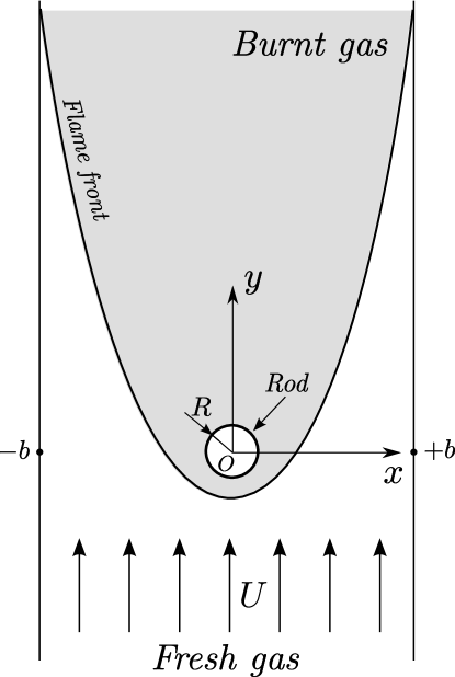
Figure 1:

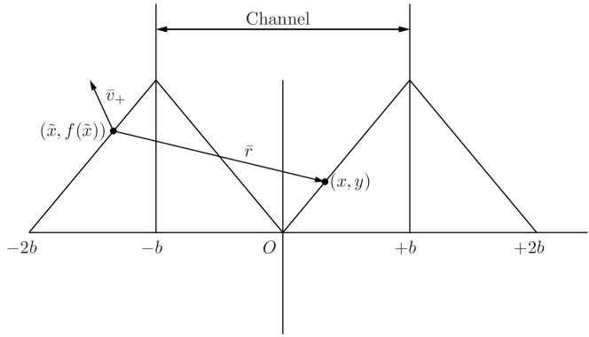
Figure 2:

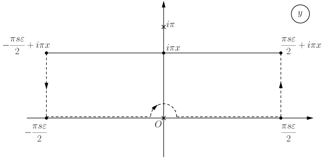
Figure 3:

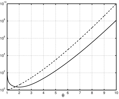
Figure 4:

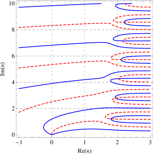
Figure 5:

References

- Scurlock (1948) A. C. Scurlock (1948), meteor Report no. 19, Massachusetts Institute of Technology.
- pro (1949) Report UMR-33 (Aeronautical research center, University of Michigan, 1949).
- Zel’dovich et al. (1985) Y. B. Zel’dovich, G. I. Barenblatt, V. B. Librovich, and G. M. Makhviladze, Mathematical Theory of Combustion and Explosions (Plenum Press, New York, 1985), chapter 6.
- Kazakov (2005a) K. A. Kazakov, Phys. Rev. Lett. 94, 094501 (2005a).
- Kazakov (2005b) K. A. Kazakov, Phys. Fluids 17, 032107 (2005b).
- El-Rabii et al. (2008) H. El-Rabii, G. Joulin, and K. A. Kazakov, Phys. Rev. Lett. 100, 174501 (2008).
- Joulin et al. (2008) G. Joulin, H. El-Rabii, and K. A. Kazakov, J. Fluid Mech. 608, 217 (2008).
- Matalon and Matkowsky (1982) M. Matalon and B. J. Matkowsky, J. Fluid Mech. 124, 239 (1982).
- Pelce and Clavin (1982) P. Pelce and P. Clavin, J. Fluid Mech. 124, 219 (1982).
- Darrieus (1938) G. Darrieus (1938), unpublished work presented at La Technique Moderne, Paris.
- Landau (1944) L. D. Landau, Acta Physicochimica USSR 19, 77 (1944).
- Sivashinsky (1977) G. I. Sivashinsky, Acta. Astron. 4, 1177 (1977).
- Sivashinsky and Clavin (1987) G. I. Sivashinsky and P. Clavin, J. Phys. (Paris) 48, 193 (1987).
- Frankel (1990) M. L. Frankel, Phys. Fluids A2, 1879 (1990).
- El-Rabii et al. (2009) H. El-Rabii, G. Joulin, and K. A. Kazakov (2009).
- Bedat and Cheng (1996) B. Bedat and R. K. Cheng, Combustion and Flame 107, 13 (1996).
- Cheng et al. (1999) R. K. Cheng, B. Bedat, and L. W. Kostiuk, Combustion and Flame 116, 360 (1999).