Smoothing splines estimators for functional linear regression

Abstract

The paper considers functional linear regression, where scalar responses $Y_{1},\ldots,Y_{n}$ are modeled in dependence of random functions $X_{1},\ldots,X_{n}$. We propose a smoothing splines estimator for the functional slope parameter based on a slight modification of the usual penalty. Theoretical analysis concentrates on the error in an out-of-sample prediction of the response for a new random function $X_{n+1}$. It is shown that rates of convergence of the prediction error depend on the smoothness of the slope function and on the structure of the predictors. We then prove that these rates are optimal in the sense that they are minimax over large classes of possible slope functions and distributions of the predictive curves. For the case of models with errors-in-variables the smoothing spline estimator is modified by using a denoising correction of the covariance matrix of discretized curves. The methodology is then applied to a real case study where the aim is to predict the maximum of the concentration of ozone by using the curve of this concentration measured the preceding day.

, and

Functional linear regression, functional parameter, functional variable, smoothing splines

1 Introduction

In a number of important applications the outcome of a response variable $Y$ depends on the variation of an explanatory variable $X$ over time (or age, etc.). An example is the application motivating our study: the data consist in repeated measurements of pollutant indicators in the area of Toulouse over the course of a day that are used to explain the maximum (peak) of pollution for the next day. Generally, a linear regression model linking observations $Y_{i}$ of a response variable with $p$ repeated measures of an explanatory variable may be written in the form

$$Y_{i}=\alpha_{0}+\frac{1}{p}\sum_{j=1}^{p}\alpha_{j}X_{i}(t_{j})+\varepsilon_{i}^{*},\qquad i=1,\ldots,n.$$ (1)

Here $t_{1}<\cdots<t_{p}$ denote observation points which are assumed to belong to a compact interval $I\subset\mathbb{R}$. The possibly varying strength of the influence of $X_{i}$ at each measurement point $t_{j}$ is quantified by different coefficients $\alpha_{j}$. Frequently $p\gg n$ and/or there is a high degree of collinearity between the “predictors” $X_{i}(t_{j}),j=1,\ldots,p$, and standard regression methods are not applicable. In addition, (1) may incorporate a discretization error, since one will often have to assume that $Y_{i}$ also depends on unobserved time points $t$ in between the observation times $t_{j}$. As pointed out by several authors (Marx and Eilers MaEi99 , Ramsay and Silverman RaSi05 or Cuevas, Febrero and Fraiman CuFeFr02 ) the use of functional models for these settings has some advantages over discrete, multivariate approaches. Only in a functional framework is it possible to profit from qualitative assumptions like smoothness of underlying curves. Assuming square integrable functions $X_{i}$ on $I\subset\mathbb{R}$, the basic object of our study is a functional linear regression model

$$Y_{i}=\alpha_{0}+\int_{I}\alpha(t)X_{i}(t)\,dt+\varepsilon_{i},\qquad i=1,\ldots,n,$$ (2)

where $\varepsilon_{i}$’s are i.i.d. centered random errors, $\mathbb{E}(\varepsilon_{i})=0$, with variance $\mathbb{E}(\varepsilon_{i}^{2})=\sigma_{\varepsilon}^{2}$, and $\alpha$ is a square integrable functional parameter defined on $I$ that must be estimated from the pairs $(X_{i},Y_{i}),i=1,\ldots,n$. This type of regression model was first considered in Ramsay and Dalzell RaDa91 . Obviously, (2) constitutes a continuous version of (1), and both models are linked by

$$\varepsilon_{i}^{*}=d_{i}+\varepsilon_{i},\qquad\mbox{where }d_{i}=\int_{I}\alpha(t)X_{i}(t)\,dt-\frac{1}{p}\sum_{j=1}^{p}\alpha(t_{j})X_{i}(t_{j})$$ (3)

may be interpreted as a discretization error, and $\alpha(t_{j})=\alpha_{j}$.

As a consequence of developments of modern technology, data that may be described by functional regression models can be found in a lot of fields such as medicine, linguistics, chemometrics (see, e.g., Ramsay and Silverman RaSi02 , RaSi05 and Ferraty and Vieu FeVi06 , for several case studies). Similarly to traditional regression problems, model (2) may arise under different experimental designs. We assume a random design of the explanatory curves, where $X_{1},\ldots,X_{n}$ is a sequence of identically distributed random functions with the same distribution as a generic $X$. The main assumption on $X$ is that it is a second-order variable, that is, $\mathbb{E}(\int_{I}X^{2}(t)\,dt)<+\infty,$ and it is assumed moreover that $\mathbb{E}(X_{i}(t)\varepsilon_{i})=0$ for almost every $t\in I$. This situation has been considered, for instance, in Cardot, Ferraty and Sarda CaFeSa03 and Müller and Stadtmüller MuSt05 for independent variables, while correlated functional variables are studied in Bosq Bo00 . Our analysis is based on a general framework without any assumption of independence of the $X_{i}$’s. We will, however, assume independence between the $X_{i}$’s and the $\varepsilon_{i}$’s in our theoretical results in Sections 3 and 4.

The main problem in functional linear regression is to derive an estimator $\widehat{\alpha}$ of the unknown slope function $\alpha$. However, estimation of $\alpha$ in (2) belongs to the class of ill-posed inverse problems. Writing (2) for generic variables $X$, $Y$ and $\varepsilon$, multiplying both sides by $X-\mathbb{E}(X)$ and then taking expectations leads to

$$\mathbb{E}\bigl{(}\bigl{(}Y-\mathbb{E}(Y)\bigr{)}\bigl{(}X-\mathbb{E}(X)\bigr{)}\bigr{)}$$

(4)

$$\qquad=\mathbb{E}\biggl{(}\int_{I}\alpha(t)\bigl{(}X(t)-\mathbb{E}(X)(t)\bigr{)}\,dt\bigl{(}X-\mathbb{E}(X)\bigr{)}\biggr{)}=:\Gamma(\alpha).$$

The normal equation (1) is the continuous equivalent of normal equations in the multivariate linear model. Estimation of $\alpha$ is thus linked with the inversion of the covariance operator $\Gamma$ of $X$ defined in (1). But, unlike the finite dimensional case, a bounded inverse for $\Gamma$ does not exist since it is a compact linear operator defined on the infinite dimensional space $L^{2}(I)$. This corresponds to the setup of ill-posed inverse problems (with the additional difficulty that $\Gamma$ is unknown). As a consequence, the parameter $\alpha$ in (2) is not identifiable without additional constraint. Actually, a necessary and sufficient condition under which a unique solution for (2)–(1) exists in the orthogonal space of $\operatorname{ker}(\Gamma)$ and is given by $\sum_{r}(\frac{\mathbb{E}((Y-\mathbb{E}(Y))\int_{I}(X(t)-\mathbb{E}(X)(t))\zeta_{r}(t)\,dt)}{\lambda_{r}})^{2}<+\infty,$ where $(\lambda_{r},\zeta_{r})_{r}$ are the eigenelements of $\Gamma$ (see Cardot, Ferraty and Sarda CaFeSa03 or He, Müller and Wang HeMuWa00 for a functional response). The set of solutions is the set of functions $\alpha$ which can be decomposed as a sum of the unique element of the orthogonal space of $\operatorname{ker}(\Gamma)$ satisfying (1) and any element of $\operatorname{ker}(\Gamma)$.

It follows from these arguments that any sensible procedure for estimating $\alpha$ (or, more precisely, of its identifiable part) has to involve regularization procedures. Several authors have proposed estimation procedures where regularization is obtained in two main ways. The first one is based on the Karhunen–Loève expansion of $X$ and leads to regression on functional principal components: see Bosq Bo00 , Cardot, Mas and Sarda CaMaSa07 or Müller and Stadtmüller MuSt05 . It consists in projecting the observations on a finite dimensional space spanned by eigenfunctions of the (empirical) covariance operator $\Gamma_{n}$. For the second method, regularization is obtained through a penalized least squares approach after expanding $\alpha$ in some basis (such as splines): see Ramsay and Dalzell RaDa91 , Eilers and Marx EiMa96 , Cardot, Ferraty and Sarda CaFeSa03 or Li and Hsing Li06 . We propose here to use a smoothing splines approach prolonging a previous work from Cardot et al. CaCrKnSa07 .

Our estimator is described in Section 2. Note that (2) implies that $Y_{i}-\overline{Y}=\int_{I}\alpha(t)[X_{i}(t)-\overline{X}(t)]\,dt+\varepsilon_{i}-\bar{\varepsilon}$. Based on the observation times $t_{1}<\cdots<t_{p}$, we rely on minimizing the residual sum of squares $\sum_{i}(Y_{i}-\overline{Y}-\frac{1}{p}\sum_{j=1}^{p}a(t_{j})(X_{i}(t_{j})-\overline{X}(t_{j})))^{2}$ subject to a roughness penalty. A slight modification of the usual penalty term is applied in order to guarantee the existence of the estimator under general conditions. The proposed estimator $\widehat{\alpha}$ is then a natural spline with knots at the observation points $t_{j}$. An estimator of the intercept $\alpha_{0}=\mathbb{E}(Y)-\int_{I}\alpha(t)\mathbb{E}(X)(t)]\,dt$ is given by $\widehat{\alpha_{0}}=\overline{Y}-\int_{I}\widehat{\alpha}(t)\overline{X}(t)\,dt$. For simplicity, we will assume that $t_{1}<\cdots<t_{p}$ are equispaced, but the methodology can easily be generalized to other situations. It must be emphasized, however, that our study does not cover the case of sparse points for which other techniques have to be envisaged; for this specific problem, see the work from Yao, Müller and Wang YaMuWa05 .

In Section 3 we present a detailed asymptotic theory of the behavior of our estimator for large values of $n$ and $p$. The distance between $\widehat{\alpha}$ and $\alpha$ is evaluated with respect to $L^{2}$ semi-norms induced by the operator $\Gamma$, $\|u\|^{2}_{\Gamma}=\langle\Gamma u,u\rangle$ with $\langle u,v\rangle=\int_{I}u(t)v(t)\,dt$, or its discretized or empirical versions (see, e.g., Cardot, Ferraty and Sarda CaFeSa03 or Müller and Stadtmüller MuSt05 for similar setups). By using these semi-norms we explicitly concentrate on analyzing the estimation error only for the identifiable part of the structure of $\alpha$ which is relevant for prediction. Indeed, it will be shown in Section 3 that $\|\widehat{\alpha}-\alpha\|_{\Gamma}^{2}$ determines the rate of convergence of the error in predicting the conditional mean $\alpha_{0}+\int_{I}\alpha(t)X_{n+1}(t)\,dt$ of $Y_{n+1}$ for any new random function $X_{n+1}$ possessing the same distribution as $X$ and independent of $X_{1},\ldots,X_{n}$:

$$\mathbb{E}\biggl{(}\biggl{(}\widehat{\alpha_{0}}+\int_{I}\widehat{\alpha}(t)X_{n+1}(t)\,dt-\alpha_{0}-\int_{I}\alpha(t)X_{n+1}(t)\,dt\biggr{)}^{2}\Big{|}\widehat{\alpha_{0}},\widehat{\alpha}\biggr{)}$$

(5)

$$\qquad=\|\widehat{\alpha}-\alpha\|_{\Gamma}^{2}+O_{P}(n^{-1}).$$

We first derived optimal rates of convergence with respect to the $L^{2}$ semi-norms induced by $\Gamma$ in a quite general setting which substantially improved existing results in the literature as well as bounds obtained for this estimator in a previous paper (see Cardot et al. CaCrKnSa07 ). If $\alpha$ is $m$-times continuously differentiable, then it is shown that rates of convergence for our estimator are of order $n^{-(2m+2q+1)/(2m+2q+2)}$, where the value of $q>0$ depends on the structure of the distribution of $X$. More precisely, $q$ quantifies the rate of decrease $\sum_{r=k+1}^{\infty}\lambda_{r}=O(k^{-2q})$ as $k\rightarrow\infty$, where $\lambda_{1}\geq\lambda_{2}\geq\cdots$ are the eigenvalues of the covariance operator $\Gamma$. If, for example, $X$ is a.s. twice continuously differentiable, then $q\geq 2$. As a second step, we show that these rates of convergence are optimal in the sense that they are minimax over large classes of distributions of $X$ and of functions $\alpha$. No alternative estimator can globally achieve faster rates of convergence in these classes.

In an interesting paper Cai and Hall CaHa06 derive rates of convergence on the error $\alpha_{0}+\langle\alpha,x\rangle-\widehat{\alpha}_{0}-\langle\widehat{\alpha},x\rangle$ for a pre-specified, fixed function $x$. Their approach is based on regression with respect to functional principal components and the derived rates are shown to be optimal with respect to this methodology. At first glance this setup seem to be close, but due to the fact that explanatory variables are of infinite dimension, inference on fixed functions $x$ cannot generally be used to derive optimal rates of convergence of the prediction error (1) for random functions $X_{n+1}$. We also want to emphasize that in the present paper we do not consider the convergence of $\hat{\alpha}$ with respect to the usual $L^{2}$ norm. Analyzing $\|\widehat{\alpha}-\alpha\|^{2}=\int_{I}(\widehat{\alpha}(t)-\alpha(t))^{2}\,dt$ instead of $\|\widehat{\alpha}-\alpha\|_{\Gamma}^{2}$ must be seen statistically as a very different problem, and under our general assumptions it only follows that $\|\widehat{\alpha}-\alpha\|^{2}$ is bounded in probability (see the proof of Theorem 2). It appears that to get stronger results one needs additional conditions linking the “smoothness” of $\alpha$ and of the curves $X_{i}$ as derived in a recent work by Hall and Horowitz HaHo07 . A detailed discussion of these issues is given in Section 3.2.

In practice the functional values $X_{i}(t_{j})$ are often not directly observed; there exist only noisy observations $W_{ij}=X_{i}(t_{j})+\delta_{ij}$ contaminated with random errors $\delta_{ij}$. In Section 4, we consider a modified functional linear model adapting to such situations. In this errors-in-variable context, we use a corrected estimator as introduced in Cardot et al. CaCrKnSa07 which can be seen as a modified version of the so-called total least squares method for functional data. We show again the good asymptotic performance of the method for a sufficiently dense grid of discretization points.

We devote Section 5 to the application of the proposed estimation procedure to the prediction of the peak of pollution from the curve of pollutant indicators collected the preceding day. Finally, the proofs of our results can be found in Section 6.

2 Smoothing splines estimation of the functional coefficient

As explained in the Introduction, we will assume that the functions $X_{i}$ are observed at $p$ equidistant points $t_{1},\ldots,t_{p}\in I$. In order to simplify further developments, we will take $I=[0,1]$ so that $t_{1}=\frac{1}{2p}$ and $t_{j}-t_{j-1}=\frac{1}{p}$ for all $j=2,\ldots,p$.

Our estimator of $\alpha$ in (2) is a generalization of the well-known smoothing splines estimator in univariate nonparametric regression. It relies on the implicit assumption that the underlying function $\alpha$ is sufficiently smooth as, for example, $m$-times continuously differentiable ($m=1,2,3,\ldots$).

For any smooth function $a$ the discrete sum $\frac{1}{p}\sum_{j=1}^{p}a(t_{j})X_{i}(t_{j})$ is used to approximate the integral $\int_{0}^{1}a(t)X_{i}(t)\,dt$ in (2), whereas expectations are estimated by the sample means $\overline{Y}$ and $\overline{X}$, and an estimate is obtained by minimizing the sum of squared residuals $(Y_{i}-\overline{Y}-\frac{1}{p}\sum_{j=1}^{p}a(t_{j})(X_{i}(t_{j})-\overline{X}(t_{j})))^{2}$ subject to a roughness penalty. More precisely, for some $m=1,2,\ldots$ and a smoothing parameter $\rho>0$, an estimate $\widehat{\alpha}$ is determined by minimizing

$$\frac{1}{n}\sum_{i=1}^{n}\Biggl{(}Y_{i}-\overline{Y}-\frac{1}{p}\sum_{j=1}^{p}a(t_{j})\bigl{(}X_{i}(t_{j})-\overline{X}(t_{j})\bigr{)}\Biggr{)}^{2}$$

(6)

$$\qquad{}+\rho\Biggl{(}\frac{1}{p}\sum_{j=1}^{p}\pi_{a}^{2}(t_{j})+\int_{0}^{1}\bigl{(}a^{(m)}(t)\bigr{)}^{2}\,dt\Biggr{)}$$

over all functions $a$ in the Sobolev space $W^{m,2}([0,1])\subset L^{2}([0,1])$, where $\pi_{a}(t)=\sum_{l=1}^{m}\beta_{a,l}t^{l-1}$ with $\sum_{j=1}^{p}(a(t_{j})-\pi_{a}(t_{j}))^{2}=\min_{\beta_{1},\ldots,\beta_{m}}\sum_{j=1}^{p}(a(t_{j})-\sum_{l=1}^{m}\beta_{l}t^{l-1})^{2}$.

Obviously, $\pi_{a}$ denotes the best possible approximation of $(a(t_{1}),\ldots,a(t_{p}))$ by a polynomial of degree $m-1$. The extra term $\frac{1}{p}\sum_{j=1}^{p}\pi_{a}(t_{j})^{2}$ in the roughness penalty is unusual and does not appear in traditional smoothing splines approaches. It will, however, be shown below that this term is necessary to guarantee existence of a unique solution in a general context without any additional assumptions on the curves $X_{i}$.

It is quite easily seen that any solution $\widehat{\alpha}$ of (2) has to be an element of the space $NS^{m}(t_{1},\ldots,t_{p})$ of natural splines of order $2m$ with knots at $t_{1},\ldots,t_{p}$. Recall that $NS^{m}(t_{1},\ldots,t_{p})$ is a $p$-dimensional linear space of functions with $v^{(m)}\in L^{2}([0,1])$ for any $v\in NS^{m}(t_{1},\ldots,t_{p})$. Let $\mathbf{b}(t)=(b_{1}(t),\ldots,b_{p}(t))^{\tau}$ be a functional basis of $NS^{m}(t_{1},\ldots,t_{p})$. A discussion of several possible basis function expansions can be found in Eubank Eu88 . An important property of natural splines is that there exists a canonical one-to-one mapping between $\mathbb{R}^{p}$ and the space $NS^{m}(t_{1},\ldots,t_{p})$ in the following way: for any vector $\mathbf{w}=(w_{1},\ldots,w_{p})^{\tau}\in\mathbb{R}^{p}$, there exists a unique natural spline interpolant $s_{\mathbf{w}}$ with $s_{\mathbf{w}}(t_{j})=w_{j}$, $j=1,\ldots,p$. With $\mathbf{B}$ denoting the $p\times p$ matrix with elements $b_{i}(t_{j})$, $s_{\mathbf{w}}$ is given by

$$s_{\mathbf{w}}(t)=\mathbf{b}(t)^{\tau}(\mathbf{B}^{\tau}\mathbf{B})^{-1}\mathbf{B}^{\tau}\mathbf{w}.$$ (7)

The important property of such a spline interpolant is the fact that

$$\int_{0}^{1}s_{\mathbf{w}}^{(m)}(t)^{2}\,dt\leq\int_{0}^{1}f^{(m)}(t)^{2}\,dt$$ (8)

$$\eqntext{\mbox{for any other function }f\in W^{m,2}([0,1])}$$ (9)

$$\eqntext{\mbox{ with }f(t_{j})=w_{j},j=1,\ldots,p.}$$ (10)

Note that in (2) only the integral $\int_{0}^{1}a^{(m)}(t)^{2}\,dt$ depends on the values of $a$ in the open intervals $(t_{j-1},t_{j})$ between grid points. It therefore follows from (8) that $\widehat{\alpha}=s_{\widehat{\bolds{\alpha}}}$, where $\widehat{\bolds{\alpha}}=(\widehat{\alpha}(t_{1}),\ldots,\widehat{\alpha}(t_{p}))^{\tau}\in\mathbb{R}^{p}$ minimizes

$$\frac{1}{n}\sum_{i=1}^{n}\Biggl{(}Y_{i}-\overline{Y}-\frac{1}{p}\sum_{j=1}^{p}a(t_{j})\bigl{(}X_{i}(t_{j})-\overline{X}(t_{j})\bigr{)}\Biggr{)}^{2}$$

(11)

$$\qquad{}+\rho\Biggl{(}\frac{1}{p}\sum_{j=1}^{p}\pi_{a}^{2}(t_{j})+\int_{0}^{1}s_{\mathbf{a}}^{(m)}(t)^{2}\,dt\Biggr{)};$$

with respect to all vectors $\mathbf{a}=(a(t_{1}),\ldots,a(t_{p}))^{\tau}\in\mathbb{R}^{p}$.

A closer study of $\widehat{\bolds{\alpha}}$ requires the use of matrix notation: $\mathbf{Y}=(Y_{1}-\overline{Y},\ldots,Y_{n}-\overline{Y})^{\tau}$, $\mathbf{X}_{i}=(X_{i}(t_{1})-\overline{X}(t_{1}),\ldots,X_{i}(t_{p})-\overline{X}(t_{p}))^{\tau}$ for all $i=1,\ldots,n$, $\bolds{\alpha}=(\alpha(t_{1}),\ldots,\alpha(t_{p}))^{\tau}$, $\bolds{\varepsilon}=(\varepsilon_{1}-\overline{\varepsilon},\ldots,\varepsilon_{n}-\overline{\varepsilon})^{\tau}$ and let $\mathbf{X}$ be the $n\times p$ matrix with a general term $X_{i}(t_{j})-\overline{X}(t_{j})$ for all $i=1,\ldots,n$,$j=1,\ldots,p$. Moreover, $\mathbf{P}_{m}$ will denote the $p\times p$ projectionmatrix projecting into the $m$-dimensional linear space $E_{m}:=\{\mathbf{w}=(w_{1},\ldots,\break w_{p})^{\tau}\in\mathbb{R}^{p}|w_{j}=\sum_{l=1}^{m}\theta_{l}t_{j}^{l-1}$, $j=1,\ldots,p\}$ of all (discretized) polynomials of degree $m-1$. By (7), we have $\int_{0}^{1}s_{\mathbf{a}}^{(m)}(t)^{2}\,dt=\mathbf{a}^{\tau}\mathbf{A}_{m}^{*}\mathbf{a}$, where $\mathbf{A}_{m}^{*}=\mathbf{B}(\mathbf{B}^{\tau}\mathbf{B})^{-1}[\int_{0}^{1}\mathbf{b}^{(m)}(t)\mathbf{b}^{(m)}(t)^{\tau}\,dt](\mathbf{B}^{\tau}\mathbf{B})^{-1}\mathbf{B}^{\tau}$ is a $p\times p$ matrix.

When defining $\mathbf{A}_{m}:=\mathbf{P}_{m}+p\mathbf{A}_{m}^{*}$, minimizing (2) is equivalent to solving

$$\min_{\mathbf{a}\in\mathbb{R}^{p}}\biggl{\{}\frac{1}{n}\biggl{\|}\mathbf{Y}-\frac{1}{p}\mathbf{X}\mathbf{a}\biggr{\|}^{2}+\frac{\rho}{p}\mathbf{a}^{\tau}\mathbf{A}_{m}\mathbf{a}\biggr{\}},$$ (12)

where $\|\cdot\|$ stands for the usual Euclidean norm. The solution is given by

$$\qquad\widehat{\bolds{\alpha}}=\frac{1}{np}\biggl{(}\frac{1}{np^{2}}\mathbf{X}^{\tau}\mathbf{X}+\frac{\rho}{p}\mathbf{A}_{m}\biggr{)}^{-1}\mathbf{X}^{\tau}\mathbf{Y}=\frac{1}{n}\biggl{(}\frac{1}{np}\mathbf{X}^{\tau}\mathbf{X}+\rho\mathbf{A}_{m}\biggr{)}^{-1}\mathbf{X}^{\tau}\mathbf{Y}.$$ (13)

Then $\widehat{\alpha}=s_{\widehat{\bolds{\alpha}}}$ constitutes our final estimator of $\alpha$ while $\widehat{\alpha_{0}}=\overline{Y}-\langle\widehat{\alpha},\overline{X}\rangle$ is used to estimate the intercept $\alpha_{0}$. Based on a somewhat different development, this estimator of $\alpha$ has already been proposed by Cardot et al. CaCrKnSa07 .

In order to verify existence of $\widehat{\bolds{\alpha}}$, let us first cite some properties of the eigenvalues of $p\mathbf{A}_{m}^{*}$ which have been studied by many authors (see Eubank Eu88 ). For instance, in Utreras Ut83 , it is shown that this matrix has exactly $m$ zero eigenvalues $\mu_{1,p}=\cdots=\mu_{m,p}=0$. The corresponding $m$-dimensional eigenspace is the space $E_{m}$ of discretized polynomials as defined above. The $p-m$ nonzero eigenvalues $0<\mu_{m+1,p}<\cdots<\mu_{p,p}$ are such that there exist constants $0<D_{0}<D_{1}<\infty$ such that $D_{0}\leq\mu_{j+m,p}(\pi j)^{-2m}\leq D_{1}$ for $j=1,\ldots,p-m$ and all sufficiently large $p$. Therefore, there exist some constant $0<C_{0}<+\infty$ and some $p_{0}\in\{0,1,2,\ldots\}$ such that for all $p\geq p_{0}$ and $k=0,\ldots,p-m-1$

$$k^{2m}\frac{1}{\mu_{k+m+1,p}}\leq C_{0}.$$ (14)

We can conclude that all eigenvalues of the matrix $\mathbf{A}_{m}$ are strictly positive, and existence as well as uniqueness of the solution (13) of the minimization problem (12) are straightforward consequences. Note that Introduction of the additional term $\frac{1}{p}\sum_{j=1}^{p}\pi_{a}(t_{j})^{2}$ in (2) is crucial. Dropping this term in (2) as well as (2) results in replacing $\mathbf{A}_{m}$ by $p\mathbf{A}_{m}^{*}$ in (12). Existence of a solution then cannot be guaranteed in a general context since, due to the $m$ zero eigenvalues of $p\mathbf{A}_{m}^{*}$, the matrix $(\frac{1}{np^{2}}\mathbf{X}^{\tau}\mathbf{X}+\rho\mathbf{A}_{m}^{*})$ may not be invertible.

Our requirement of equidistant grid points $t_{j}$ has to be seen as a restrictive condition. There are many applications where the functions $X_{i}$ are only observed at varying numbers $p_{i}$ of irregularly spaced points $t_{i1}\leq\cdots\leq t_{ip_{i}}$. Then our estimation procedure is not directly applicable. Fortunately there exists a fairly simple modification. Define a smooth function $\widetilde{X}_{i}\in L^{2}([0,1])$ by smoothly interpolating the observations (e.g., using natural splines) such that $\widetilde{X}_{i}(t_{ij})=X_{i}(t_{ij})$, $j=1,\ldots,p_{i}$. Then define $p>\max\{p_{1},\ldots,p_{n}\}$ equidistant grid points $t_{1},\ldots,t_{p}$, and determine an estimator $\widehat{\alpha}$ by applying the smoothing spline procedure (2) with $\frac{1}{p}\sum_{j=1}^{p}a(t_{j})(X_{i}(t_{j})-\overline{X}(t_{j}))$ being replaced by $\frac{1}{p}\sum_{j=1}^{p}a(t_{j})(\widetilde{X}_{i}(t_{j})-\overline{\widetilde{X}}(t_{j}))$. For example, in the case of a random design with i.i.d. observations $t_{ij}$ from a strictly positive design density on $I$, it may be shown that the asymptotic results of Section 3 generalize to this situation if $\min\{p_{1},\ldots,$ $p_{n}\}$ is sufficiently large compared to $n$. A detailed analysis is not in the scope of the present paper.

3 Theoretical results

3.1 Rates of convergence for smoothing splines estimators

We will denote the standard inner product of the Hilbert space $L^{2}([0,1])$ by $\langle f,g\rangle=\int_{0}^{1}f(t)g(t)\,dt$ and $\|\cdot\|$ by its associated norm. As outlined in the Introduction, our analysis is based on evaluating the error between $\widehat{\alpha}$ and $\alpha$ with respect to the semi-norm $\|\cdot\|_{\Gamma}$ defined in Section 1,

$$\|u\|_{\Gamma}^{2}:=\langle\Gamma u,u\rangle,\qquad u\in L^{2}([0,1]),$$

where $\Gamma$ is the covariance operator of $X$ given by

$$\Gamma u:=\mathbb{E}\bigl{(}\bigl{\langle}\bigl{(}X-\mathbb{E}(X)\bigr{)},u\bigr{\rangle}\bigl{(}X-\mathbb{E}(X)\bigr{)}\bigr{)},\qquad u\in L^{2}([0,1]).$$

The above $L^{2}$ semi-norm has already been used in similar contexts as the one studied in the present paper; see, for example, Wahba Wa77 , Cardot, Ferraty and Sarda CaFeSa03 or Müller and Stadtmüller MuSt05 . By (1) the asymptotic behavior of $\|\widehat{\alpha}-\alpha\|_{\Gamma}^{2}$ constitutes a major object of interest, since it quantifies the leading term in the expected squared prediction error for a new random function $X_{n+1}$.

As first steps, we will consider in Theorems 1 and 2 the error between $\widehat{\alpha}$ and $\alpha$ with respect to simplified versions of the above semi-norm: the discretized empirical semi-norm defined for any $\mathbf{u}\in\mathbb{R}^{p}$ as

$$\|\mathbf{u}\|_{\Gamma_{n,p}}^{2}:=\frac{1}{p}\mathbf{u}^{\tau}\biggl{(}\frac{1}{np}\mathbf{X}^{\tau}\mathbf{X}\biggr{)}\mathbf{u},$$

and the empirical semi-norm defined for any $u\in L^{2}([0,1])$ as

$$\|u\|_{\Gamma_{n}}^{2}:=\frac{1}{n}\sum_{i=1}^{n}\langle(X_{i}-\overline{X}),u\rangle^{2}=\langle\Gamma_{n}u,u\rangle,$$

where $\Gamma_{n}$ is the empirical covariance operator from $X_{1},\ldots,X_{n}$ given by

$$\Gamma_{n}u:=\frac{1}{n}\sum_{i=1}^{n}\langle(X_{i}-\overline{X}),u\rangle(X_{i}-\overline{X}).$$

Obviously, $\|\widehat{\bolds{\alpha}}-\bolds{\alpha}\|_{\Gamma_{n,p}}^{2}=\frac{1}{n}\sum_{i}[\frac{1}{p}\sum_{j=1}^{p}(\widehat{\alpha}(t_{j})-\alpha(t_{j}))(X_{i}(t_{j})-\overline{X}(t_{j}))]^{2}$ and $\|\widehat{\alpha}-\alpha\|_{\Gamma_{n}}^{2}=\frac{1}{n}\sum_{i}[\int_{I}(\widehat{\alpha}(t)-\alpha(t))(X_{i}(t)-\overline{X}(t))\,dt]^{2}$ quantify different modes of convergence of $\langle\widehat{\alpha},X-\overline{X}\rangle$ to $\langle\alpha,(X-\overline{X})\rangle$.

As mentioned in Section 2, the function $\alpha$ is required to have a certain degree of regularity. Namely, it satisfies the following assumption for some $m\in\{1,2,\ldots\}$:

$$\alpha\mbox{ is $m$-times differentiable and $\alpha^{(m)}$ belongs to $L^{2}([0,1])$.}$$ (A.1)

Let $C_{1}=\int_{0}^{1}\alpha^{(m)}(t)^{2}\,dt$ and $C_{2}^{*}=\int_{0}^{1}\alpha(t)^{2}\,dt$. By construction of $\mathbf{P}_{m}$, $\mathbf{P}_{m}\bolds{\alpha}$ provides the best approximation (in a least squares sense) of $\bolds{\alpha}$ by (discretized) polynomials of degree $m-1$, and $\frac{1}{p}\bolds{\alpha}^{\tau}\mathbf{P}_{m}\bolds{\alpha}\leq\frac{1}{p}\bolds{\alpha}^{\tau}\mathbf{A}_{m}\bolds{\alpha}\longrightarrow C_{2}^{*}$ as $p\rightarrow\infty$. Let $C_{2}$ denote an arbitrary constant with $C_{2}^{*}<C_{2}<\infty$. There then exists a $p_{1}\in\{0,1,\ldots\}$ with $p_{1}\geq p_{0}$ such that $\frac{1}{p}\bolds{\alpha}^{\tau}\mathbf{P}_{m}\bolds{\alpha}\leq C_{2}$ for all $p\geq p_{1}$.

Recall that our basic setup implies that $X_{1},\ldots,X_{n}$ are identically distributed random functions with the same distribution as a generic variable $X$. Expected values $\mathbb{E}_{\varepsilon}(\cdot)$ as stated in the theorems below will refer to the probability distribution induced by the random variable $\varepsilon$, that is, they stand for conditional expectation given $X_{1},\ldots,X_{n}$. We assume moreover that $\varepsilon_{i}$ is independent of the $X_{i}$’s. In the following, for any real positive number $x$, $[x]$ will denote the smallest integer which is larger than $x$. In addition, let $\lambda_{x,1}\geq\lambda_{x,2}\geq\cdots\geq\lambda_{x,p}\geq 0$ denote the eigenvalues of the matrix $\frac{1}{np}\mathbf{X}^{\tau}\mathbf{X}$. We start with a theorem giving finite sample bounds for bias and variance of the estimator $\widehat{\bolds{\alpha}}$ with respect to the semi-norm $\|\cdot\|_{\Gamma_{n,p}}$.

Theorem 1

Under assumption (A.1) and the above definitions of $C_{0}$, $C_{1}$, $C_{2}$, $p_{1}$, the following bounds hold for all $n=0,1,\ldots,$ all $p\geq p_{1}$, all $\rho>n^{-2m}$ and every $n\times p$ matrix $\mathbf{X}=(X_{i}(t_{j}))_{i,j}$:

$$\|\mathbb{E}_{\varepsilon}(\widehat{\bolds{\alpha}})-\bolds{\alpha}\|_{\Gamma_{n,p}}^{2} \leq 2\rho\biggl{(}\frac{1}{p}\bolds{\alpha}^{\tau}\mathbf{P}_{m}\bolds{\alpha}+C_{1}\biggr{)}+\frac{4}{n}\sum_{i=1}^{n}(d_{i}-\overline{d})^{2}$$

$$\leq \rho(C_{2}+C_{1})+\frac{4}{n}\sum_{i=1}^{n}(d_{i}-\overline{d})^{2},$$

as well as

$$\mathbb{E}_{\varepsilon}\bigl{(}\|\widehat{\bolds{\alpha}}-\mathbb{E}_{\varepsilon}(\widehat{\bolds{\alpha}})\|_{\Gamma_{n,p}}^{2}\bigr{)}\leq\frac{\sigma^{2}_{\varepsilon}}{n}\Bigl{(}m+\bigl{[}\rho^{-{1}/({2m+2q+1})}\bigr{]}(2+C\cdot C_{0})\Bigr{)},$$ (3.2)

for any $C>0$ and $q\geq 0$ with the property that $\sum_{j=k+1}^{p}\lambda_{x,j}\leq C\cdot k^{-2q}$ holds for $k:=[\rho^{-{1}/({2m+2q+1})}]$.

The rate of convergence of $\|\widehat{\bolds{\alpha}}-\bolds{\alpha}\|_{\Gamma_{n,p}}^{2}$ thus depends on assumptions on the distribution of $X$ and on the size of the discretization error. In order to complement our basic setup, we will rely on the following conditions:

1. [(A.2)]

2. There exists some constant $\kappa$, $0<\kappa<1,$ such that for every $\delta>0$, there exists a constant $C_{3}<+\infty$ such that

   $$\mathbb{P}\bigl{(}|X(t)-X(s)|\leq C_{3}|t-s|^{\kappa},t,s\in I\bigr{)}\geq 1-\delta.$$

3. For some constant $C_{4}<\infty$ and all $k=1,2,\ldots$ there is a $k$-dimensional linear subspace $\mathcal{L}_{k}$ of $L^{2}([0,1])$ with

   $$\mathbb{E}\biggl{(}\inf_{f\in\mathcal{L}_{k}}\sup_{t}|X(t)-f(t)|^{2}\biggr{)}\leq C_{4}k^{-2q}.$$

Before proceeding any further, let us consider assumption (A.3) more closely. The following lemma provides a link between assumption (A.3) and the degree of smoothness of the random functions $X_{i}$.

Lemma 1

For some $q_{1}=0,1,2,\ldots$ and $0\leq r_{2}\leq 1$ assume that $X$ is almost surely $q_{1}$-times continuously differentiable and that there exists some $C_{5}<\infty$ such that

$$\mathbb{E}\biggl{(}\sup_{|t-s|\leq d}\bigl{|}X^{(q_{1})}(t)-X^{(q_{1})}(s)\bigr{|}^{2}\biggr{)}\leq C_{5}d^{2r_{2}}$$

holds for all $d>0$. There then exists a constant $C_{6}<\infty$, depending only on $q_{1}$, such that for all $k=1,2,\ldots$

$$\mathbb{E}\biggl{(}\inf_{f\in\mathcal{E}_{k}}\sup_{t}|X(t)-f(t)|^{2}\biggr{)}\leq C_{6}C_{5}k^{-2(q_{1}+r_{2})},$$

where $\mathcal{E}_{k}$ denotes the space of all polynomials of order $k$ on $[0,1]$.

The well-known Jackson’s inequality in approximation theory implies the existence of some $C_{6}<\infty$, only depending on $q_{1}$, such that for all $k=1,2,\ldots$

$$\inf_{f\in\mathcal{E}_{k}}\sum_{j=1}^{p}\bigl{(}X(t_{j})-f(t_{j})\bigr{)}^{2}\leq C_{6}k^{-2q_{1}}\sup_{|t-s|\leq 1/k}\bigl{|}X^{(q_{1})}(t)-X^{(q_{1})}(s)\bigr{|}^{2}$$

holds with probability 1. The lemma is an immediate consequence.

The lemma implies that if assumption (A.2) can be replaced by the stronger requirement $\mathbb{E}(\sup_{|t-s|\leq d}|X(t)-X(s)|^{2})\leq C_{5}d^{-2r_{2}}$, $d>0$, then assumption (A.3) necessarily holds for some $q\geq\kappa$. Indeed, $q\gg\kappa$ will result from a very high degree of smoothness of $X_{i}$.

On the other hand, assumption (A.3) only requires that the functions $X_{i}$ be well approximated by some arbitrary low dimensional linear function spaces (not necessarily polynomials). Even if $X_{i}$ are not smooth, assumption (A.3) may be satisfied for a large value of $q$ (the Brownian motion provides an example).

Theorem 1 together with assumptions (A.2) and (A.3) now allows us to derive rates of convergence of our estimator $\widehat{\alpha}$. First note that assumption (A.3) determines the rate of decrease of the eigenvalues $\lambda_{x,j}$ of $\frac{1}{np}\mathbf{X}^{\tau}\mathbf{X}$. For any $k$-dimensional linear space $\mathcal{L}_{k}\subset L^{2}([0,1])$, let $\mathcal{P}_{k}$ denote the corresponding $p\times p$ projection matrix projecting into the $k$-dimensional subspace $\mathcal{L}_{k,p}=\{v\in\mathbb{R}^{p}|v=(f(t_{1}),\ldots,f(t_{p}))^{\tau},f\in\mathcal{L}_{k}\}$. Basic properties of eigenvalues and eigenvectors then imply that

$$\sum_{j=k+1}^{p}\lambda_{x,j}\leq\inf_{\mathcal{P}_{k}}\operatorname{Tr}\biggl{(}(\mathbf{I}_{p}-\mathcal{P}_{k})\frac{1}{np}\mathbf{X}^{\tau}\mathbf{X}\biggr{)}$$

(3.3)

$$\qquad=\frac{1}{np}\sum_{i=1}^{n}\inf_{f\in\mathcal{L}_{k}}\sum_{j=1}^{p}\bigl{(}X_{i}(t_{j})-\overline{X}-f(t_{j})\bigr{)}^{2},$$

and assumption (A.3) implies that for any $\delta>0$ there exists a $C_{\delta}<\infty$ such that $P(\sum_{j=k+1}^{p}\lambda_{x,j}\leq C_{\delta}k^{-2q})\geq 1-\delta$.

Assumptions (A.1) and (A.2) obviously lead to

$$\frac{1}{n}\sum_{i=1}^{n}(d_{i}-\overline{d})^{2}=O_{P}(p^{-2\kappa}).$$ (3.4)

If $n,p\rightarrow\infty$, $\rho\rightarrow 0$, $1/(n\rho)\rightarrow 0$, then relations (1), (3.2) and (3.1) imply that

$$\|\widehat{\bolds{\alpha}}-\bolds{\alpha}\|_{\Gamma_{n,p}}^{2}=O_{P}\bigl{(}\rho+\bigl{(}n\rho^{{1}/({2m+2q+1})}\bigr{)}^{-1}+p^{-2\kappa}\bigr{)}.$$

In the following we will require that $p$ is sufficiently large compared to $n$ so that the discretization error is negligible. It therefore suffices that $np^{-2\kappa}=O(1)$ as $n,p\rightarrow\infty$. This condition imposes a large number $p$ of observation points if $\kappa$ is small. However, if the functions $X_{i}$ are smooth enough such that $\kappa=1,$ then $np^{-2\kappa}=O(1)$ is already fulfilled if $\frac{\sqrt{n}}{p}=O(1)$ as $n,p\rightarrow\infty$, which does not seem to be restrictive in view of practical applications. The above result then becomes

$$\|\widehat{\bolds{\alpha}}-\bolds{\alpha}\|_{\Gamma_{n,p}}^{2}=O_{P}\bigl{(}\rho+\bigl{(}n\rho^{{1}/({2m+2q+1})}\bigr{)}^{-1}\bigr{)}.$$ (3.5)

Choosing $\rho\sim n^{-(2m+2q+1)/(2m+2q+2)}$, we can conclude that

$$\|\widehat{\bolds{\alpha}}-\bolds{\alpha}\|_{\Gamma_{n,p}}^{2}=O_{P}\bigl{(}n^{-(2m+2q+1)/(2m+2q+2)}\bigr{)}.$$ (3.6)

The next theorem studies the behavior of the estimator for the empirical $L^{2}$-norm $\|\cdot\|_{\Gamma_{n}}$. It is shown that if $p$ is sufficiently large compared to $n$, then based on an optimal choice of $\rho$, the rate of convergence given in (3.6) generalizes to the semi-norm $\|\cdot\|_{\Gamma_{n}}$.

Theorem 2

Assume (A.1)–(A.3) as well as $np^{-2\kappa}=O(1)$, $\rho\rightarrow 0$, $1/\break(n\rho)\rightarrow 0$ as $n,p\rightarrow\infty$. Then

$$\|\widehat{\alpha}-\alpha\|_{\Gamma_{n}}^{2}=O_{P}\bigl{(}\rho+\bigl{(}n\rho^{{1}/({2m+2q+1})}\bigr{)}^{-1}\bigr{)}.$$ (3.7)

We finally investigate in the next theorem the behavior of $\|\widehat{\alpha}-\alpha\|_{\Gamma}^{2}$. The following assumption describes the additional conditions used to derive our results. It is well known that the covariance operator $\Gamma$ is a nuclear, self-adjoint and nonnegative Hilbert–Schmidt operator. We will use $\zeta_{1},\zeta_{2},\ldots$ to denote a complete orthonormal system of eigenfunctions of $\Gamma$ corresponding to the eigenvalues $\lambda_{1}\geq\lambda_{2}\geq\cdots$.

(A.4) There exists a constant $C_{7}<\infty$ such that

$$\operatorname{Var}\Biggl{(}\frac{1}{n}\sum_{i}\langle X_{i}-\mathbb{E}(X),\zeta_{r}\rangle\langle X_{i}-\mathbb{E}(X),\zeta_{s}\rangle\Biggr{)}$$

(3.8)

$$\qquad\leq\frac{C_{7}}{n}\mathbb{E}\bigl{(}\langle X-\mathbb{E}(X),\zeta_{r}\rangle^{2}\bigr{)}\mathbb{E}\bigl{(}\langle X-\mathbb{E}(X),\zeta_{s}\rangle^{2}\bigr{)}$$

holds for all $n$ and all $r,s=1,2,\ldots.$ Moreover, $\|\overline{X}-\mathbb{E}(X))\|^{2}=O_{P}(n^{-1})$.

Relation (3.1) establishes a moment condition. It is necessarily fulfilled if $X_{1},\ldots,X_{n}$ are i.i.d. Gaussian random functions. Then $\langle X_{i}-\mathbb{E}(X),\zeta_{r}\rangle\sim N(0,\mathbb{E}(\langle X_{i}-\mathbb{E}(X),\zeta_{r}\rangle^{2}))$, and $\langle X_{i}-\mathbb{E}(X),\zeta_{r}\rangle$ is independent of $\langle X_{i}-\mathbb{E}(X),\zeta_{s}\rangle$ if $r\neq s$. Relation (3.1) then is an immediate consequence.

However, the validity of (3.1) does not require independence of the functions $X_{i}$. For example, in the Gaussian case, (3.1) may also be verified if $\operatorname{Cov}(\langle X_{i}-\mathbb{E}(X),\zeta_{r}\rangle\langle X_{i}-\mathbb{E}(X),\zeta_{s}\rangle,\langle X_{j}-\mathbb{E}(X),\zeta_{r}\rangle\langle X_{j}-\mathbb{E}(X),\zeta_{s}\rangle)\leq C_{7}\mathbb{E}(\langle X_{i}-\mathbb{E}(X),\zeta_{r}\rangle^{2})\mathbb{E}(\langle X_{i}-\mathbb{E}(X),\zeta_{s}\rangle^{2})\cdot q^{|i-j|}$ for some $0<q<1$, $C_{7}<\infty$ and $i\neq j$. This is of importance in our application to ozone pollution forecasting which deals with a time series of functions $X_{1},\ldots,X_{n}$.

Theorem 3

Under the conditions of Theorem 2 together with assumption (A.4) we have

$$\|\widehat{\alpha}-\alpha\|_{\Gamma}^{2}=O_{P}\bigl{(}\rho+\bigl{(}n\rho^{{1}/({2m+2q+1})}\bigr{)}^{-1}+n^{-(2q+1)/2}\bigr{)}.$$ (3.9)

Furthermore, (1) holds for any random function $X_{n+1}$ possessing the same distribution as $X$ and independent of $X_{1},\ldots,X_{n}$.

Theorem 3 shows that if $2q\geq 1$ and $\rho\sim n^{-(2m+2q+1)/(2m+2q+2)}$, then the prediction error can be bounded by

$$\mathbb{E}\bigl{(}(\widehat{\alpha_{0}}+\langle\widehat{\alpha},X_{n+1}\rangle-\alpha_{0}-\langle\alpha,X_{n+1}\rangle)^{2}|\widehat{\alpha_{0}},\widehat{\alpha}\bigr{)}=O_{P}\bigl{(}n^{-({2m+2q+1})/({2m+2q+2})}\bigr{)}.$$

3.2 Optimality of the rates of convergence

For simplicity we will rely on the special case of (2) with $\alpha_{0}=0$. In this case $\mathbb{E}((\langle\alpha,X_{n+1}\rangle-\widehat{\alpha_{0}}-\langle\widehat{\alpha},X_{n+1}\rangle)^{2}|\widehat{\alpha_{0}},\widehat{\alpha})\geq\|\widehat{\alpha}-\alpha\|_{\Gamma}^{2}$ if $X$ possesses a centered distribution with $\mathbb{E}(X)=0$. In Proposition 1 below we then show that for suitable Sobolev spaces of functions $\alpha$ and a large class of possible distributions of $X_{i}$, the rate $n^{-(2m+2q+1)/(2m+2q+2)}$ is a lower bound for the rate of convergence of the prediction error over all estimators of $\alpha$ to be computed from corresponding observations $(X_{i},Y_{i})$, $i=1,\ldots,n$. Consequently, the rate attained by our smoothing spline estimator $\widehat{\alpha}$ must be interpreted as a minimax rate over these classes.

We first have to introduce some additional notation. For simplicity, we will assume that the functions $X_{i}(t)$ are known for all $t$ so that the number $p$ of observation points may be chosen arbitrarily large. We will use $\mathcal{C}_{m,D}$ to denote the space of all $m$-times continuously differentiable functions $\alpha$ with $\int_{0}^{1}\alpha^{(j)}(t)^{2}\,dt\leq D$ for all $j=0,1,\ldots,m$. Furthermore, let $\mathcal{P}_{q,C}$ denote the space of all centered probability distributions on $L^{2}([0,1])$ with the properties that (a) the sequence of eigenvalues of the corresponding covariance operator satisfies $\sum_{j=k+1}^{\infty}\lambda_{j}\leq Ck^{-2q}$ for all sufficiently large $k$, and that (b) the smoothing spline estimator $\widehat{\alpha}$ satisfies $\|\widehat{\alpha}-\alpha\|_{\Gamma}^{2}=O_{P}(n^{-(2m+2q+1)/(2m+2q+2)})$ for $\alpha\in\mathcal{C}_{m,D}$ and $\rho\sim n^{-(2m+2q+1)/(2m+2q+2)}$ (whenever $p$ is chosen sufficiently large compared to $n$). Finally, for given $\alpha\in\mathcal{C}_{m,D}$, probability distribution $P\in\mathcal{P}_{q,C}$ and i.i.d. random functions $X_{1},\ldots,X_{n}$, $X_{i}\sim P$, let $\hat{a}(\alpha,P)$ denote an arbitrary estimator of $\alpha$ based on corresponding data $(X_{i},Y_{i})$, $i=1,\ldots,n$, generated by (2) (with $\alpha_{0}=0$).

Proposition 1

Let $c_{n}$ denote an arbitrary sequence of positive numbers with $c_{n}\rightarrow 0$ as $n\rightarrow\infty$, and let $2q=1,3,5,\ldots.$ Under the above assumptions, we have

$$\lim\limits_{n\rightarrow\infty}\sup\limits_{P\in\mathcal{P}_{q,C}}\sup\limits_{\alpha\in\mathcal{C}_{m,D}}\inf\limits_{\hat{a}(\alpha,P)}\mathbb{P}\bigl{(}\|\alpha-\hat{a}(\alpha,P)\|^{2}_{\Gamma}\geq c_{n}\cdot n^{-(2m+2q+1)/(2m+2q+2)}\bigr{)}=1.$$

It is of interest to compare our results with those of Cai and Hall CaHa06 who analyze the error $\langle\alpha-\widehat{\alpha},x\rangle^{2}$ for a fixed curve $x$. Similarly to our results, the rate of decrease of the eigenvalues $\lambda_{r}$ of $\Gamma$ plays an important role. Note that, as shown in the proof of Theorem 3, assumption (A.3) yields $\sum_{r=k+1}^{\infty}\lambda_{r}=O(k^{-2q})$. Since $\lambda_{1}\geq\lambda_{2}\geq\cdots$ this in turn implies that $\lambda_{r}=O(r^{-2q-1})$, and one may reasonably assume that $B^{-1}r^{-2q-1}\leq\lambda_{r}\leq Br^{-2q-1}$ for some $0<B<\infty$. However, Cai and Hall CaHa06 measure “smoothness” of $\alpha$ in terms of a spectral decomposition $\alpha(t)=\sum_{r}\alpha_{r}\zeta_{r}(t)$ and not with respect to usual smoothness classes. Their quantity of interest is the rate $\beta>1$ of decrease $|\alpha_{r}|=O(r^{-\beta})$ as $r\rightarrow\infty$. But recall that the error in expanding an $m$-times continuously differentiable function with respect to $k$ suitable basis functions (as, e.g., orthogonal polynomials or Fourier functions) is of an order of at most $k^{-2m}$. For the sake of comparison, assume that $\zeta_{1},\zeta_{2},\ldots$ define an appropriate basis for approximating smooth functions and that $\inf_{f\in\operatorname{span}\{\zeta_{1},\ldots,\zeta_{k}\}}\|\alpha-f\|^{2}=\sum_{r=k+1}^{\infty}\alpha_{r}^{2}=O(k^{-2m})$. This will require that $\alpha_{r}^{2}=O(r^{-2m-1})$ and, hence, $2\beta=2m+1$.

Results as derived by Cai and Hall CaHa06 additionally depend on the spectral decomposition $x(t)=\sum_{r}x_{r}\zeta_{r}(t)$ of a function $x$ of interest. The essential condition on the structure of the coefficients $x_{r}$ may be re-expressed in the following form: There exist some $\nu\in\mathbb{R}$ and $0<D_{0}<\infty$ such that $D_{0}^{-1}r^{\nu}\leq\frac{x_{r}^{2}}{\lambda_{r}}\leq D_{0}r^{\nu}$ for all $r=1,2,\ldots.$ Rates of convergence then follow from the magnitude of $\nu$, and it is shown that parametric rates $n^{-1}$ (or $n^{-1}\log n$) are achieved if $\nu\leq-1$.

Now consider a random function $X_{n+1}$ and assume that the underlying distribution is Gaussian. It is then well known that $X_{n+1}(t)=\sum_{r}x_{n+1,r}\zeta_{r}(t)$ for independent $N(0,\lambda_{r})$-distributed coefficients $x_{n+1,r}$. Consequently, $\frac{x_{n+1,r}^{2}}{\lambda_{r}}$ are i.i.d. $\chi_{1}^{2}$-distributed variables for all $r=1,2,\ldots,$ and if $\nu\leq 0$ we obtain $\mathbb{P}(D_{0}^{-1}r^{\nu}\leq\frac{x_{n+1,r}^{2}}{\lambda_{r}}\leq D_{0}r^{\nu}\mbox{ for all }r=1,2,\ldots)=0$ for all $0<D_{0}<\infty$. This already shows that parametric rates $n^{-1}$ cannot be achieved for the error $\langle\alpha-\widehat{\alpha},X_{n+1}\rangle^{2}$. On the other hand, for arbitrary $\nu>0$ and $0<\delta<1$ we have $\mathbb{P}(D_{0}^{-1}r^{\nu}\leq\frac{x_{n+1,r}^{2}}{\lambda_{r}}\leq D_{0}r^{\nu}\mbox{ for all }r=1,2,\ldots)\geq\delta$, whenever $D_{0}$ is sufficiently large. If $B^{-1}r^{-2q-1}\leq\lambda_{r}\leq Br^{-2q-1}$ and $\alpha_{r}^{2}=O_{P}(r^{-2m+1})$, then for a function $x$ with $D_{0}^{-1}r^{\nu}\leq\frac{x_{n+1,r}^{2}}{\lambda_{r}}\leq D_{0}r^{\nu}$, $\nu>0$, the convergence rates of Cai and Hall CaHa06 translate into

$$\langle\widehat{\alpha}-\alpha,x\rangle^{2}=O_{P}\bigl{(}n^{-(2m+2q+1-2\nu)/(2m+2q+2)}\bigr{)},$$

which provides an additional motivation for the fact that the rates derived in our paper constitute a lower bound. For non-Gaussian distributions a comparison is more difficult, since under assumption (A.4) only the Chebyshev inequality may be used to bound the probabilities $D_{0}^{-1}r^{\nu}\leq\frac{x_{n+1,r}^{2}}{\lambda_{r}}\leq D_{0}r^{\nu}$.

Another statistically very different problem consists in an optimal estimation of $\alpha$ by $\widehat{\alpha}$ with respect to the usual $L^{2}$-norm. In a recent work, Hall and Horowitz HaHo07 derive optimal rates of convergence of $\|\widehat{\alpha}-\alpha\|^{2}$. These rates again depend on the rate of decrease $|\alpha_{r}|=O(r^{-\beta})$. Recall that our assumptions do not provide any link between $\alpha$ and $X_{i}$; part of the structure of $\alpha$ may not even be identifiable. Indeed, under assumptions (A.1)–(A.4) there is no way to guarantee that the bias $\|\alpha-\mathbb{E}_{\varepsilon}(\widehat{\alpha})\|^{2}$ converges to zero and it can only be shown that $\|\widehat{\alpha}-\alpha\|^{2}=O_{P}(1)$ (see the proof of Theorem 2 below). This already highlights the theoretical difference between optimal estimation with respect to $\|\widehat{\alpha}-\alpha\|_{\Gamma}^{2}$ and $\|\widehat{\alpha}-\alpha\|^{2}$. Based on additional assumptions as indicated above, although sensible bounds for the bias may be derived, it must be emphasized that an estimator minimizing $\|\widehat{\alpha}-\alpha\|^{2}$ will have to rely on $\rho\gg n^{-(2m+2q+1)/(2m+2q+2)}$, which corresponds to an oversmoothing with respect to $\|\widehat{\alpha}-\alpha\|_{\Gamma}^{2}$. This effect has already been noted by Cai and Hall CaHa06 . In our context, without additional assumptions linking the eigenvalues of $\Gamma$ and of the spline matrix $\mathbf{A}_{m}$, the only general bound for the $L_{2}$-variability of the estimator is $\|\widehat{\alpha}-\mathbb{E}_{\varepsilon}(\widehat{\alpha})\|^{2}=O_{P}(\frac{1}{n\rho})$ (this result may be derived by arguments similar to those used in the proofs of our theorems). With $\rho=n^{-(2m+2q+1)/(2m+2q+2)}$ this leads to $\|\widehat{\alpha}-\mathbb{E}_{\varepsilon}(\widehat{\alpha})\|^{2}=O_{P}(n^{-1/(2m+2q+2)})$, and better rates may only be achieved with $\rho\gg n^{-(2m+2q+1)/(2m+2q+2)}$. A more detailed study of this problem is not in the scope of the present paper.

3.3 Choice of smoothing parameters

The above result of Section 3.1 implies that the choice of the smoothing parameter $\rho$ is of crucial importance. A natural way to determine $\rho$ is to minimize a leave-one-out cross-validation criterion. We preferably adapt the simplified Generalized Cross-Validation (GCV) introduced by Wahba Wa90 in the context of smoothing splines. For fixed $m$, in our application the GCV criterion takes the form

$$\mathit{GCV}_{m}(\rho):=\frac{({1}/{n})\|\mathbf{Y}-\mathbf{H}_{\rho}\mathbf{Y}\|^{2}}{(1-n^{-1}\operatorname{Tr}(\mathbf{H}_{\rho}))^{2}},$$ (3.10)

where $\mathbf{H}_{\rho}:=(np)^{-1}\mathbf{X}(\frac{1}{np^{2}}\mathbf{X}^{\tau}\mathbf{X}+\frac{\rho}{p}\mathbf{A}_{m})^{-1}\mathbf{X}^{\tau}$.

Proposition 2 below provides a justification for the use of the GCV criterion. Recall that the estimators $\widehat{\bolds{\alpha}}\equiv\widehat{\bolds{\alpha}}_{\rho;m}$ depend on $\rho$ as well as on the spline order $m$. Obviously, $\frac{1}{p}\mathbf{X}\widehat{\bolds{\alpha}}_{\rho;m}=\mathbf{H}_{\rho}\mathbf{Y}$ is an estimator of the conditional mean $(\langle X_{1}-\overline{X},\alpha\rangle,\ldots,\langle X_{n}-\overline{X},\alpha\rangle)^{\tau}$ of $\mathbf{Y}$ given $X_{1},\ldots,X_{n}$. Let

$$\mathit{ASE}_{m}(\rho):=\frac{1}{n}\sum_{i}\Biggl{[}\langle X_{i}-\overline{X},\alpha\rangle-\frac{1}{p}\sum_{j}\bigl{(}X_{i}(t_{j})-\overline{X}(t_{j})\bigr{)}\hat{\alpha}_{\rho;m}(t_{j})\Biggr{]}^{2}$$

denote the average squared error of this estimator. The only difference between $\mathit{ASE}_{m}(\rho)$ and $\|\widehat{\bolds{\alpha}}_{\rho}-\bolds{\alpha}\|_{\Gamma_{n,p}}^{2}$ is the discretization error encountered when approximating $\langle X_{i},\alpha\rangle$ by $\frac{1}{p}\sum_{j}X_{i}(t_{j})\alpha(t_{j})$, and hence $\mathit{ASE}_{m}(\rho)=\|\widehat{\bolds{\alpha}}_{\rho}-\bolds{\alpha}\|_{\Gamma_{n,p}}^{2}+O_{P}(p^{-2\kappa})$.

If $\hat{\rho}$ denotes the minimizer of GCV for fixed $m$, we can conclude from relation (3.11) of Proposition 2 that the error $\mathit{ASE}_{m}(\hat{\rho})$ is asymptotically first-order equivalent to the error $\mathit{ASE}_{m}(\rho_{\mathrm{opt}})$ to be obtained from an optimal choice of the smoothing parameter. Furthermore, (3.12) shows that an analogous result holds if GCV is additionally used to select the order $m$ of the smoothing spline, which means that the optimal rate can be reached adaptively.

Proposition 2

In addition to assumptions (A.1)–(A.3) as well as $np^{-2\kappa}=O(1),$ suppose that $\mathbb{E}(\exp(\beta\varepsilon_{i}^{2}))<\infty$ for some $\beta>0$. If for fixed $m$, $\hat{\rho}$ denotes the minimizer of $\mathit{GCV}(\rho)$ over $\rho\in[n^{-2m+\delta},\infty)$ for some $\delta>0$, then

$$|\mathit{ASE}_{m}(\hat{\rho})-\mathit{ASE}_{m}(\rho_{\mathrm{opt}})|=O_{P}\bigl{(}n^{-{1}/{2}}\mathit{ASE}_{m}(\rho_{\mathrm{opt}})^{{1}/{2}}\bigr{)},$$ (3.11)

where $\rho_{\mathrm{opt}}$ minimizes $\mathit{MSE}_{m}(\rho):=\mathbb{E}_{\varepsilon}(\mathit{ASE}_{m}(\rho))$ over all $\rho>0$.

Furthermore, if $\hat{m},\hat{\rho}$ denotes the minimizers of (3.10) over $\rho\in[n^{-2m+\delta},\infty)$, $\delta>0$, and $m=1,\ldots,M_{n}$, $M_{n}\leq n/2$, then

$$\qquad|\mathit{ASE}_{\hat{m}}(\hat{\rho})-\mathit{ASE}_{m_{\mathrm{opt}}}(\rho_{\mathrm{opt}})|=O_{P}(n^{-{1}/{2}}\mathit{ASE}_{m_{\mathrm{opt}}}(\rho_{\mathrm{opt}})^{{1}/{2}}\log M_{n}),$$ (3.12)

where $\rho_{\mathrm{opt}},m_{\mathrm{opt}}$ minimize $\mathit{MSE}_{m}(\rho):=\mathbb{E}_{\varepsilon}(\mathit{ASE}_{m}(\rho))$ over all $\rho>0$ and $m=1,\ldots,M_{n}$.

4 Case of a noisy covariate

In a number of important applications measurements of the explanatory curves $X_{i}$ may be contaminated by noise. There then additionally exists an errors-in-variable problem complicating further analysis. Our setup is inspired by other works dealing with noisy observations of functional data (e.g., Cardot Ca00 or Chiou, Müller and Wang ChMuWa03 ): At each point $t_{j}$ the corresponding functional value $X_{i}(t_{j})$ is corrupted by some random error $\delta_{ij}$ so that actual observations $W_{i}(t_{j})$ are given by

$$W_{i}(t_{j})=X_{i}(t_{j})+\delta_{ij},\qquad i=1,\ldots,n,j=1,\ldots,p,$$ (4.13)

where $(\delta_{ij})_{i=1,\ldots,n,j=1,\ldots,p}$ is a sequence of independent real random variables such that for all $i=1,\ldots,n$ and all $j=1,\ldots,p$

$$\mathbb{E}_{\varepsilon}(\delta_{ij})=0,\qquad\mathbb{E}_{\varepsilon}(\delta_{ij}^{2})=\sigma_{\delta}^{2}\quad\mbox{and}\quad\mathbb{E}_{\varepsilon}(\delta_{ij}^{4})\leq C_{8}$$ (4.14)

for some constant $C_{8}>0$ (independent of $n$ and $p$). We furthermore assume that $\delta_{ij}$ is independent of $\varepsilon_{i}$ and of the $X_{i}$’s.

In this situation, an analogue of our estimator $\widehat{\alpha}$ of Section 2 can still be computed by replacing in (13) the (unknown) matrix $\mathbf{X}$ by the $n\times p$ matrix $\mathbf{W}$ with general terms $W_{i}(t_{j})-\overline{W}$, $i=1,\ldots,n$, $j=1,\ldots,p$. However, performance of the resulting estimator will suffer from the additional noise in the observations. If the error variance $\sigma^{2}_{\delta}$ is large, there may exist a substantial difference between $\mathbf{X}^{\tau}\mathbf{X}$ and $\mathbf{W}^{\tau}\mathbf{W}$. Indeed, $\mathbf{W}^{\tau}\mathbf{W}$ is a biased estimator of $\mathbf{X}^{\tau}\mathbf{X}$:

$$\frac{1}{np^{2}}\mathbf{W}^{\tau}\mathbf{W}=\frac{1}{np^{2}}\mathbf{X}^{\tau}\mathbf{X}+\frac{\sigma_{\delta}^{2}}{p^{2}}\mathbf{I}_{p}+\mathbf{R},$$ (4.15)

where $\mathbf{R}$ is a $p\times p$ matrix such that its largest singular value is of order $O_{P}(\frac{1}{n^{1/2}p})$, (see the proof of Theorem 4 below). This result suggests that we use $\frac{1}{np^{2}}\mathbf{W}^{\tau}\mathbf{W}-\frac{\sigma_{\delta}^{2}}{p^{2}}\mathbf{I}_{p}$ as an approximation of $\frac{1}{np^{2}}\mathbf{X}^{\tau}\mathbf{X}$. A prerequisite is, of course, the availability of an estimator $\hat{\sigma}_{\delta}^{2}$ of the unknown variance $\sigma_{\delta}^{2}$. Following Gasser, Sroka and Jennen-Steinmetz GaSrSt86 , we will rely on

$$\quad\widehat{\sigma}_{\delta}^{2}:=\frac{1}{n}\sum_{i=1}^{n}\frac{1}{6(p-2)}\sum_{j=2}^{p-1}[W_{i}(t_{j-1})-W_{i}(t_{j})+W_{i}(t_{j+1})-W_{i}(t_{j})]^{2}.$$ (4.16)

These arguments now lead to the following modified estimator $\widehat{\bolds{\alpha}}_{\mathbf{W}}$ of $\bolds{\alpha}$ in the case of noisy observations:

$$\widehat{\bolds{\alpha}}_{\mathbf{W}}:=\frac{1}{np}\biggl{(}\frac{1}{np^{2}}\mathbf{W}^{\tau}\mathbf{W}+\frac{\rho}{p}\mathbf{A}_{m}-\frac{\widehat{\sigma}_{\delta}^{2}}{p^{2}}\mathbf{I}_{p}\biggr{)}^{-1}\mathbf{W}^{\tau}\mathbf{Y}.$$ (4.17)

An estimator of the function $\alpha$ is given by $\widehat{\alpha}_{\mathbf{W}}=s_{\widehat{\bolds{\alpha}}_{\mathbf{W}}}$, where $s_{\widehat{\bolds{\alpha}}_{\mathbf{W}}}$ is again the natural spline interpolant of order $2m$ as defined in Section 2.

We want to note that $\widehat{\bolds{\alpha}}_{\mathbf{W}}$ is closely related to an estimator proposed by Cardot et al. CaCrKnSa07 . The latter is motivated by the Total Least Squares (TLS) method (see, e.g., Golub and Van Loan GoVanLo80 , Fuller Fu87 , or Van Huffel and Vandewalle VanHuVa91 ) and the only difference from (4.17) consists in the use of a correction term slightly different from $-\frac{\widehat{\sigma}_{\delta}^{2}}{p^{2}}\mathbf{I}_{p}$.

Of course there are many alternative strategies for dealing with the errors-in-variable problem induced by (4.13). A straightforward approach, which is frequently used in functional data analysis, is to apply nonparametric smoothing procedures in order to obtain estimates $\hat{X}_{i}(t_{j})$ from the data $(W_{i}(t_{j}),t_{j})$. When replacing $\mathbf{X}$ by $\widehat{\mathbf{X}}$ in (13), one can then define a “smoothed” estimator $\widehat{\bolds{\alpha}}_{S}$. Of course this estimator may be as efficient as (4.17), but it is computationally more involved and appropriate smoothing parameters have to be selected for nonparametric estimation of each curve $X_{i}$.

Our aim is now to study the asymptotic behavior of $\widehat{\alpha}_{\mathbf{W}}$. Theorem 4 below provides bounds (with respect to the semi-norm $\Gamma_{n,p}$) for the difference between $\widehat{\bolds{\alpha}}_{\mathbf{W}}$ and the “ideal” estimator $\widehat{\bolds{\alpha}}$ defined for the true curves $X_{1},\ldots,X_{n}$. We will impose the following additional condition on the function $\alpha$:

1. [(A.5)]

2. For every $\delta>0$ there exists a constant $C_{\alpha}<\infty$ such that

   $$\frac{1}{p^{1/2}}\biggl{\|}\frac{1}{np}\mathbf{X}^{\tau}\mathbf{X}\bolds{\alpha}\biggr{\|}>C_{\alpha},$$

   holds with probability larger or equal to $1-\delta$.

Theorem 4

Assume (A.1), (A.2), (A.5) as well as $np^{-2\kappa}=O(1)$, $\rho\rightarrow 0$, $1/(n\rho)\rightarrow 0$ as $n,p\rightarrow\infty$. Then

$$\|\widehat{\bolds{\alpha}}_{\mathbf{W}}-\widehat{\bolds{\alpha}}\|_{\Gamma_{n,p}}^{2}=O_{P}\biggl{(}\frac{1}{np\rho}+\frac{1}{n}\biggr{)}.$$ (4.18)

Together with assumption (A.3) we can therefore conclude from Theorems 1 and 4 that

$$\|\widehat{\bolds{\alpha}}_{\mathbf{W}}-\bolds{\alpha}\|_{\Gamma_{n,p}}^{2}=O_{P}\biggl{(}\rho+\bigl{(}n\rho^{{1}/({2m+2q+1})}\bigr{)}^{-1}+\frac{1}{np\rho}\biggr{)}.$$

We have already seen in Section 3 that the optimal order of the two first terms is reached for a choice of $\rho\sim n^{-(2m+2q+1)/(2m+2q+2)}$. From an asymptotic point of view, the use of $\widehat{\alpha}_{\mathbf{W}}$ results in the addition of the extra term $1/(np\rho)$ in the rate of convergence. For $\rho\sim n^{-(2m+2q+1)/(2m+2q+2)}$ we have $1/(np\rho)\sim n^{-1/(2m+2q+2)}/p$. This term is of order $n^{-(2m+2q+1)/(2m+2q+2)}$ for $p\sim n^{(2m+2q-1)/(2m+2q+2)}$. This means that the $\widehat{\alpha}_{\mathbf{W}}$ reaches the same rate of convergence as $\widehat{\bolds{\alpha}}$ provided that $p$ is sufficiently large compared to $n$. More precisely, it is required that $p\geq C_{p}\max(n^{1/2\kappa},n^{(2m+2q-1)/(2m+2q+2)})$ for some positive constant $C_{p}$.

As shown in Theorem 5 below, these qualitative results generalize when considering the semi-norms $\Gamma_{n}$ or $\Gamma$.

Theorem 5

Assume (A.1)–(A.3), (A.5) as well as $np^{-2\kappa}=O(1)$, $\rho\rightarrow 0$, $1/(n\rho)\rightarrow 0$ as $n,p\rightarrow\infty$. Then

$$\|\widehat{\alpha}_{\mathbf{W}}-\widehat{\alpha}\|_{\Gamma_{n}}^{2}=O_{P}\biggl{(}\frac{1}{np\rho}+\frac{1}{n}\biggr{)},$$ (4.19)

and if assumption (A.4) is additionally satisfied,

$$\|\widehat{\alpha}_{\mathbf{W}}-\widehat{\alpha}\|_{\Gamma}^{2}=O_{P}\biggl{(}\frac{1}{np\rho}+\frac{1}{n}+n^{-(2q+1)/2}\biggr{)}.$$ (4.20)

5 Application to ozone pollution forecasting

In this section, our methodology is applied to the problem of predicting the level of ozone pollution. For our analysis, we use a data set collected by ORAMIP (Observatoire R gional de l’Air en Midi-Pyr n es), an air observatory located in the city of Toulouse (France). The concentration of specific pollutants as well as meteorological variables are measured each hour. Some previous studies using the same data are described in Cardot, Crambes and Sarda CaCrSa06 and Aneiros-Perez et al. AnCaEsVi04 .

The response variable $Y_{i}$ of interest is the maximum of ozone for a day. Repeated measurements of ozone concentration obtained for the preceding day are used as a functional explicative variable $X_{i}$. More precisely, each $X_{i}$ is observed at $p=24$ equidistant points corresponding to hourly measurements. The sample size is $n=474$. It is assumed that the relation between $Y_{i}$ and $X_{i}$ can be modeled by the functional linear regression model (2). We note at this point that $X_{1},X_{2},\ldots$ constitute a time series of functions, and that it is therefore reasonable to suppose some correlation between the $X_{i}$’s. The results of an earlier, unpublished study indicate that there only exists some “short memory” dependence.

Now, for a curve $X_{n+1}$ outside the sample, we want to predict $Y_{n+1}$, the maximum of ozone the day after. Assuming that $(X_{n+1},Y_{n+1})$ follows the same model (2) and using our estimators $\widehat{\alpha}$ of $\alpha$ and $\widehat{\alpha_{0}}$ of $\alpha_{0}$ described in Section 2, a predictor $\widehat{Y}_{n+1}$ is given by the formula

$$\widehat{Y}_{n+1}:=\widehat{\alpha_{0}}+\int_{I}\widehat{\alpha}(t)X_{n+1}(t)\,dt.$$ (5.21)

It cannot be excluded that actual observations of $X_{i}$ may be contaminated with noise. We will thus additionally consider the modified estimator $\widehat{\alpha}_{\mathbf{W}}$ developed in Section 4 and the corresponding predictor $\widehat{Y}_{\mathbf{W},n+1}$. For simplicity, the integral in (5.21) is approximated by $\frac{1}{p}\sum_{j=1}^{p}\widehat{\alpha}(t_{j})X_{n+1}(t_{j})$. With additional assumptions on the $\varepsilon_{i}$’s we can also build asymptotic intervals of prediction for $Y_{n+1}$. Indeed, let us assume that $\varepsilon_{1},\ldots,\varepsilon_{n+1}$ are i.i.d. random variables having a normal distribution $\mathcal{N}(0,\sigma_{\varepsilon}^{2})$. The first point is to estimate the residual variance $\sigma_{\varepsilon}^{2}$. A straightforward estimator is given by the empirical variance

$$\widehat{\sigma_{\varepsilon}}^{2}:=\frac{1}{n}\sum_{i=1}^{n}\Biggl{(}Y_{i}-\overline{Y}-\frac{1}{p}\sum_{j=1}^{p}\widehat{\alpha}(t_{j})\bigl{(}X_{i}(t_{j})-\overline{X}(t_{j})\bigr{)}\Biggr{)}^{2}.$$ (5.22)

Our theoretical results imply that $\widehat{\sigma_{\varepsilon}}$ is a consistent estimator of $\sigma_{\varepsilon}^{2}$. Furthermore, we can then infer from Theorem 3 that $\frac{Y_{n+1}-\widehat{Y}_{n+1}}{\widehat{\sigma_{\varepsilon}}}$ asymptotically follows a standard normal distribution. Given $\tau\in\,]0,1[$, an asymptotic $(1-\tau)$-prediction interval for $Y_{n+1}$ can be derived as

$$[\widehat{Y}_{n+1}-z_{1-\tau/2}\widehat{\sigma_{\varepsilon}},\widehat{Y}_{n+1}+z_{1-\tau/2}\widehat{\sigma_{\varepsilon}}],$$ (5.23)

where $z_{1-\tau/2}$ is the quantile of order $1-\tau/2$ of the $\mathcal{N}(0,1)$ distribution. Of course, the same developments are valid when one replaces $\widehat{Y}_{n+1}$ by $\widehat{Y}_{\mathbf{W},n+1}$.

In order to study performance of our estimators we split the initial sample into two sub-samples:

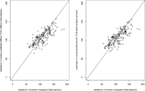
Figure 1: Daily predicted values $\widehat{Y}$ (left) and $\widehat{Y}_{\mathbf{W}}$ (right) of the maximum of ozone versus the measured values.

• A learning sample, $(X_{i},Y_{i})_{i=1,\ldots,n_{l}}$, $n_{l}=300$, was used to determine the estimators $\widehat{\alpha}$ and $\widehat{\alpha}_{\mathbf{W}}$.

• A test sample, $(X_{i},Y_{i})_{i=n_{l}+1,\ldots,n_{l}+n_{t}}$, $n_{t}=174$, was used to evaluate the quality of the estimation.

Construction of estimators was based on $m=2$ (cubic smoothing splines), and the smoothing parameters $\rho$ were selected by minimizing $\mathit{GCV}(\rho)$ as defined in (3.10). Note that GCV for $\widehat{\alpha}_{\mathbf{W}}$ requires that the matrix $\frac{1}{np^{2}}\mathbf{X}^{\tau}\mathbf{X}$ in the definition of $\mathbf{H}_{\rho}$ has to be replaced by $\frac{1}{np^{2}}\mathbf{W}^{\tau}\mathbf{W}-\frac{\widehat{\sigma}_{\delta}^{2}}{p^{2}}\mathbf{I}_{p}$. Figure 1 presents the daily predicted values $\widehat{Y}$ and $\widehat{Y}_{\mathbf{W}}$ of the maximum of ozone versus the measured $Y$-values of the test sample. Both graphics are close, which is confirmed by the computation of the prediction error given by

$$\mathit{EQM}(\widehat{\alpha}):=\frac{1}{n_{t}}\sum_{i=n_{l}+1}^{n_{l}+n_{t}}(Y_{i}-\widehat{Y}_{i})^{2},$$

with a similar definition for $\widehat{\alpha}_{\mathbf{W}}$. We have, respectively, $\mathit{EQM}(\widehat{\alpha})=281.97$ and $\mathit{EQM}(\widehat{\alpha}_{\mathbf{W}})=270.13,$ which shows a very minor advantage of the estimator $\widehat{\alpha}_{\mathbf{W}}$. In any case, in Figure 1 the points seem to be reasonably spread around the diagonal $\hat{Y}=Y$, and the plots do not indicate any major problem with our estimators. Corresponding prediction intervals are given in Figure 2.

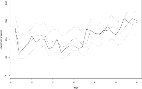
Figure 2: Measured values of the maximum of ozone (solid line), predicted values (dashed line) and $95\%$ prediction band (dotted lines).

6 Proof of the results

6.1 Proof of Theorem 1

First consider relation (1), and note that

$$\mathbb{E}_{\varepsilon}(\widehat{\bolds{\alpha}})=\frac{1}{np^{2}}\biggl{(}\frac{1}{np^{2}}\mathbf{X}^{\tau}\mathbf{X}+\frac{\rho}{p}\mathbf{A}_{m}\biggr{)}^{-1}\mathbf{X}^{\tau}\mathbf{X}\bolds{\alpha}+\frac{1}{np}\biggl{(}\frac{1}{np^{2}}\mathbf{X}^{\tau}\mathbf{X}+\frac{\rho}{p}\mathbf{A}_{m}\biggr{)}^{-1}\mathbf{X}^{\tau}\mathbf{d},$$

where $\mathbf{d}=(d_{1}-\overline{d},\ldots,d_{n}-\overline{d})^{\tau}$.

It follows that $\mathbb{E}_{\varepsilon}(\widehat{\bolds{\alpha}})$ is a solution of the minimization problem

$$\min_{\mathbf{a}\in\mathbb{R}^{p}}\biggl{\{}\frac{1}{n}\biggl{\|}\frac{1}{p}\mathbf{X}\bolds{\alpha}+\mathbf{d}-\frac{1}{p}\mathbf{X}\mathbf{a}\biggr{\|}^{2}+\frac{\rho}{p}\mathbf{a}^{\tau}\mathbf{A}_{m}\mathbf{a}\biggr{\}}.$$

This implies

$$\frac{1}{n}\biggl{\|}\frac{1}{p}\mathbf{X}\bolds{\alpha}+\mathbf{d}-\frac{1}{p}\mathbf{X}\mathbb{E}_{\varepsilon}(\widehat{\bolds{\alpha}})\biggr{\|}^{2}+\frac{\rho}{p}\mathbb{E}_{\varepsilon}(\widehat{\bolds{\alpha}})^{\tau}\mathbf{A}_{m}\mathbb{E}_{\varepsilon}(\widehat{\bolds{\alpha}})\leq\frac{\rho}{p}\bolds{\alpha}^{\tau}\mathbf{A}_{m}\bolds{\alpha}+\frac{1}{n}\|\mathbf{d}\|^{2}.$$

But definition of $\mathbf{A}_{m}$ and (8) lead to

$$\frac{1}{p}\bolds{\alpha}^{\tau}\mathbf{A}_{m}\bolds{\alpha}=\frac{1}{p}\bolds{\alpha}^{\tau}\mathbf{P}_{m}\bolds{\alpha}+\int_{0}^{1}s_{\bolds{\alpha}}^{(m)}(t)^{2}\,dt\leq\frac{1}{p}\bolds{\alpha}^{\tau}\mathbf{P}_{m}\bolds{\alpha}+\int_{0}^{1}\alpha^{(m)}(t)^{2}\,dt$$

and (1) is an immediate consequence. Let us now consider relation (3.2). There exists a complete orthonormal system of eigenvectors $u_{1},u_{2},\ldots,u_{p}$ of $\frac{1}{np}\mathbf{X}^{\tau}\mathbf{X}$ such that $\frac{1}{np}\mathbf{X}^{\tau}\mathbf{X}=\sum_{j=1}^{p}\lambda_{x,j}u_{j}u_{j}^{\tau}$. Let $k:=[\rho^{-{1}/({2m+2q+1})}]$. By our assumptions we obtain

$$\mathbb{E}_{\varepsilon}\bigl{(}\|\widehat{\bolds{\alpha}}-\mathbb{E}_{\varepsilon}(\widehat{\bolds{\alpha}})\|_{\Gamma_{n,p}}^{2}\bigr{)}$$

$$\qquad=\frac{1}{p}\mathbb{E}_{\varepsilon}\biggl{(}\frac{1}{n^{2}p^{2}}\bolds{\varepsilon}^{\tau}\mathbf{X}\biggl{(}\frac{1}{np^{2}}\mathbf{X}^{\tau}\mathbf{X}+\frac{\rho}{p}\mathbf{A}_{m}\biggr{)}^{-1}$$

$$\hskip 59.1pt{}\times\frac{1}{np}\mathbf{X}^{\tau}\mathbf{X}\biggl{(}\frac{1}{np^{2}}\mathbf{X}^{\tau}\mathbf{X}+\frac{\rho}{p}\mathbf{A}_{m}\biggr{)}^{-1}\mathbf{X}^{\tau}\bolds{\varepsilon}\biggr{)}$$

$$\qquad\leq\frac{\sigma_{\varepsilon}^{2}}{n}\operatorname{Tr}\biggl{[}\biggl{(}\frac{1}{np}\mathbf{X}^{\tau}\mathbf{X}+\rho\mathbf{A}_{m}\biggr{)}^{-1}\frac{1}{np}\mathbf{X}^{\tau}\mathbf{X}\biggr{]}$$ (6.24)

$$\qquad=\frac{\sigma_{\varepsilon}^{2}}{n}\operatorname{Tr}\biggl{[}\biggl{(}(\rho\mathbf{A}_{m})^{-{1}/{2}}\biggl{(}\frac{1}{np}\mathbf{X}^{\tau}\mathbf{X}\biggr{)}(\rho\mathbf{A}_{m})^{-{1}/{2}}+\mathbf{I}_{p}\biggr{)}^{-1}$$

$$\hskip 99.0pt{}\times(\rho\mathbf{A}_{m})^{-{1}/{2}}\biggl{(}\frac{1}{np}\mathbf{X}^{\tau}\mathbf{X}\biggr{)}(\rho\mathbf{A}_{m})^{-{1}/{2}}\biggr{]}$$

$$\qquad\leq\frac{\sigma_{\varepsilon}^{2}}{n}\operatorname{Tr}(\mathbf{D}_{1,\rho}+\mathbf{D}_{2,\rho}),$$

where

$$\mathbf{D}_{1,\rho}:\! = \Biggl{(}(\rho\mathbf{A}_{m})^{-{1}/{2}}\Biggl{(}\sum_{j=1}^{k}\lambda_{x,j}u_{j}u_{j}^{\tau}\Biggr{)}(\rho\mathbf{A}_{m})^{-{1}/{2}}+\mathbf{I}_{p}\Biggr{)}^{-1}$$

$${}\times(\rho\mathbf{A}_{m})^{-{1}/{2}}\Biggl{(}\sum_{j=1}^{k}\lambda_{x,j}u_{j}u_{j}^{\tau}\Biggr{)}(\rho\mathbf{A}_{m})^{-{1}/{2}}$$

and

$$\mathbf{D}_{2,\rho}:\! = \Biggl{(}(\rho\mathbf{A}_{m})^{-{1}/{2}}\Biggl{(}\sum_{j=k+1}^{p}\lambda_{x,j}u_{j}u_{j}^{\tau}\Biggr{)}(\rho\mathbf{A}_{m})^{-{1}/{2}}+\mathbf{I}_{p}\Biggr{)}^{-1}$$

$${}\times(\rho\mathbf{A}_{m})^{-{1}/{2}}\Biggl{(}\sum_{j=k+1}^{p}\lambda_{x,j}u_{j}u_{j}^{\tau}\Biggr{)}(\rho\mathbf{A}_{m})^{-{1}/{2}}$$

which are symmetric $p\times p$ matrices with

$$\sup_{\|\mathbf{v}\|=1}\mathbf{v}^{\tau}\mathbf{D}_{1,\rho}\mathbf{v}<1\quad\mbox{and}\quad\sup_{\|\mathbf{v}\|=1}\mathbf{v}^{\tau}\mathbf{D}_{2,\rho}\mathbf{v}<1.$$ (6.25)

Furthermore, $\mathbf{D}_{1,\rho}$ is of rank $k$ and therefore only possesses $k$ nonzero eigenvalues. Hence

$$\operatorname{Tr}(\mathbf{D}_{1,\rho})\leq k.$$ (6.26)

Let $\mathbf{a}_{1,p},\ldots,\mathbf{a}_{m,p},\mathbf{a}_{m+1,p},\ldots,\mathbf{a}_{p,p}$ denote a complete, orthonormal system of eigenvectors of $\mathbf{A}_{m}$ corresponding to the eigenvalues $\mu_{1,p}=\cdots=\mu_{m,p}=1$ and $\mu_{m+1,p}\leq\cdots\leq\mu_{p,p}$. By (6.1), (6.25) and (6.26) as well as (14), we thus obtain

$$\mathbb{E}_{\varepsilon}\bigl{(}\|\widehat{\bolds{\alpha}}-\mathbb{E}_{\varepsilon}(\widehat{\bolds{\alpha}})\|_{\Gamma_{n,p}}^{2}\bigr{)}$$

$$\qquad\leq\frac{\sigma_{\varepsilon}^{2}}{n}\Biggl{(}k+\sum_{j=1}^{p}\mathbf{a}_{j,p}^{\tau}\mathbf{D}_{2,\rho}\mathbf{a}_{j,p}\Biggr{)}$$

$$\qquad\leq\frac{\sigma_{\varepsilon}^{2}}{n}\Biggl{(}k+m+k+\sum_{l=m+k+1}^{p}\mathbf{a}_{l,p}^{\tau}(\rho\mathbf{A}_{m})^{-{1}/{2}}$$

$$\hskip 57.0pt\hskip 91.2pt{}\times\Biggl{(}\sum_{j=k+1}^{p}\lambda_{x,j}u_{j}u_{j}^{\tau}\Biggr{)}(\rho\mathbf{A}_{m})^{-{1}/{2}}\mathbf{a}_{l,p}\Biggr{)}$$

$$\qquad\leq\frac{\sigma_{\varepsilon}^{2}}{n}\Biggl{(}m+2k+\frac{1}{\mu_{m+k+1}\cdot\rho}\sum_{j=k+1}^{p}\lambda_{x,j}\Biggr{)}$$

$$\qquad\leq\frac{\sigma_{\varepsilon}^{2}}{n}(m+2k+CkC_{0})$$

$$\qquad=\frac{\sigma_{\varepsilon}^{2}}{n}\bigl{(}m+\bigl{[}\rho^{-{1}/({2m+2q+1})}\bigr{]}\bigr{)}(2+CC_{0}).$$

This proves Relation (3.2) and completes the proof of Theorem 1.

6.2 Proof of Theorem 2

With $\widehat{d}_{i}=\int_{I}\widehat{\alpha}(t)X_{i}(t)\,dt-\frac{1}{p}\sum_{j=1}^{p}\widehat{\alpha}(t_{j})X_{i}(t_{j})$ we have

$$\|\widehat{\alpha}-\alpha\|_{\Gamma_{n}}^{2} \leq \frac{2}{n}\sum_{i=1}^{n}\Biggl{[}\langle(X_{i}-\overline{X}),\widehat{\alpha}-\alpha\rangle$$

$$\hskip 28.4pt{}-\frac{1}{p}\sum_{j=1}^{p}\bigl{(}X_{i}(t_{j})-\overline{X}(t_{j})\bigr{)}\bigl{(}\widehat{\alpha}(t_{j})-\alpha(t_{j})\bigr{)}\Biggr{]}^{2}$$

$${}+\frac{2}{n}\sum_{i=1}^{n}\Biggl{[}\frac{1}{p}\sum_{j=1}^{p}(X_{i}-\overline{X})(t_{j})\bigl{(}\widehat{\alpha}(t_{j})-\alpha(t_{j})\bigr{)}\Biggr{]}^{2}$$

$$\leq \frac{4}{n}\sum_{i=1}^{n}(\widehat{d}_{i}-\overline{\widehat{d}})^{2}+\frac{4}{n}\sum_{i=1}^{n}(d_{i}-\overline{d})^{2}+2\|\widehat{\bolds{\alpha}}-\bolds{\alpha}\|_{\Gamma_{n,p}}^{2}.$$

By assumptions (A.1)–(A.3), it follows from Theorem 1, (3.1) and (3.4) that the assertion of Theorem 2 holds, provided that

$$\frac{1}{n}\sum_{i=1}^{n}(\widehat{d}_{i}-\overline{\widehat{d}})^{2}=O_{P}(p^{-2\kappa}).$$ (6.29)

The proof of (6.29) consists of several steps. We will start by giving a stochastic bound for $\frac{1}{p}\widehat{\bolds{\alpha}}^{\tau}\widehat{\bolds{\alpha}}$ and then study the stochastic behavior of $\int_{0}^{1}\widehat{\alpha}^{(m)}(t)^{2}\,dt$. The use of a suitable Taylor expansion will then lead to the desired result.

By definition of $\widehat{\bolds{\alpha}}$ we have

$$\frac{1}{p}\widehat{\bolds{\alpha}}^{\tau}\widehat{\bolds{\alpha}} \leq \frac{3}{p}\bolds{\alpha}^{\tau}\frac{1}{np}\mathbf{X}^{\tau}\mathbf{X}\biggl{(}\frac{1}{np}\mathbf{X}^{\tau}\mathbf{X}+\rho\mathbf{A}_{m}\biggr{)}^{-2}\frac{1}{np}\mathbf{X}^{\tau}\mathbf{X}\bolds{\alpha}$$

$${}+3\frac{1}{n^{2}p}\mathbf{d}^{\tau}\mathbf{X}\biggl{(}\frac{1}{np}\mathbf{X}^{\tau}\mathbf{X}+\rho\mathbf{A}_{m}\biggr{)}^{-2}\mathbf{X}^{\tau}\mathbf{d}$$

$${}+3\frac{1}{n^{2}p}\bolds{\varepsilon}^{\tau}\mathbf{X}\biggl{(}\frac{1}{np}\mathbf{X}^{\tau}\mathbf{X}+\rho\mathbf{A}_{m}\biggr{)}^{-2}\mathbf{X}^{\tau}\bolds{\varepsilon}.$$

Since all eigenvalues of the matrix $\frac{1}{np}\mathbf{X}^{\tau}\mathbf{X}(\frac{1}{np}\mathbf{X}^{\tau}\mathbf{X}+\rho\mathbf{A}_{m})^{-2}\frac{1}{np}\mathbf{X}^{\tau}\mathbf{X}$ are less than or equal to 1, the first term on the right-hand side of (6.2) is less than or equal to $\frac{3}{p}\bolds{\alpha}^{\tau}\bolds{\alpha}=O(1)$. It is easily seen that the smallest eigenvalue of the matrix $\frac{1}{np}\mathbf{X}(\frac{1}{np}\mathbf{X}^{\tau}\mathbf{X}+\rho\mathbf{A}_{m})^{-2}\mathbf{X}^{\tau}$ is proportional to $1/\rho$, and thus the second term can be bounded by a term of order $p^{-2\kappa}/\rho$. By (14) the expected value of the third term is bounded by

$$\frac{\sigma_{\varepsilon}^{2}}{n}\operatorname{Tr}\biggl{[}\frac{1}{np}\mathbf{X}\biggl{(}\frac{1}{np}\mathbf{X}^{\tau}\mathbf{X}+\rho\mathbf{A}_{m}\biggr{)}^{-2}\mathbf{X}^{\tau}\biggr{]}\leq\frac{\sigma_{\varepsilon}^{2}}{n}\operatorname{Tr}[(\rho\mathbf{A}_{m})^{-1}]=O\bigl{(}1/(n\rho)\bigr{)}.$$

We therefore arrive at

$$\frac{1}{p}\widehat{\bolds{\alpha}}^{\tau}\widehat{\bolds{\alpha}}=O_{P}\biggl{(}1+\frac{p^{-2\kappa}}{\rho}+\frac{1}{n\rho}\biggr{)}.$$ (6.31)

As a next step we will study the asymptotic behavior of $\int_{0}^{1}\widehat{\alpha}^{(m)}(t)^{2}\,dt$. Since $\widehat{\bolds{\alpha}}$ is solution of the minimization problem (12), we can write

$$\frac{1}{n}\biggl{\|}\mathbf{Y}-\frac{1}{p}\mathbf{X}\widehat{\bolds{\alpha}}\biggr{\|}^{2}+\frac{\rho}{p}\widehat{\bolds{\alpha}}^{\tau}\mathbf{P}_{m}\widehat{\bolds{\alpha}}+\rho\int_{0}^{1}\widehat{\alpha}^{(m)}(t)^{2}\,dt$$

$$\qquad\leq\frac{1}{n}\biggl{\|}\mathbf{Y}-\frac{1}{p}\mathbf{X}\bolds{\alpha}\biggr{\|}^{2}+\frac{\rho}{p}\bolds{\alpha}^{\tau}\mathbf{P}_{m}\bolds{\alpha}+\rho\int_{0}^{1}\alpha^{(m)}(t)^{2}\,dt,$$

and therefore

$$\rho\int_{0}^{1}\widehat{\alpha}^{(m)}(t)^{2}\,dt \leq \|\widehat{\bolds{\alpha}}-\bolds{\alpha}\|_{\Gamma_{n,p}}^{2}+\frac{2}{n}\biggl{\langle}\mathbf{Y}-\frac{1}{p}\mathbf{X}\bolds{\alpha},\frac{1}{p}\mathbf{X}\widehat{\bolds{\alpha}}-\frac{1}{p}\mathbf{X}\bolds{\alpha}\biggr{\rangle}$$

$${}+\rho\int_{0}^{1}\alpha^{(m)}(t)^{2}\,dt-\frac{\rho}{p}\widehat{\bolds{\alpha}}^{\tau}\mathbf{P}_{m}\widehat{\bolds{\alpha}}+\frac{\rho}{p}\bolds{\alpha}^{\tau}\mathbf{P}_{m}\bolds{\alpha}.$$

We have to focus on the term

$$\frac{2}{n}\biggl{\langle}\mathbf{Y}-\frac{1}{p}\mathbf{X}\bolds{\alpha},\frac{1}{p}\mathbf{X}\widehat{\bolds{\alpha}}-\frac{1}{p}\mathbf{X}\bolds{\alpha}\biggr{\rangle}=\frac{2}{n}\biggl{\langle}\mathbf{d}+\bolds{\varepsilon},\frac{1}{p}\mathbf{X}\widehat{\bolds{\alpha}}-\frac{1}{p}\mathbf{X}\bolds{\alpha}\biggr{\rangle}.$$

The Cauchy–Schwarz inequality together with the definition of $\|\cdot\|_{\Gamma_{n,p}}^{2}$ yield

$$\frac{1}{n}\mathbf{d}^{\tau}\biggl{(}\frac{1}{p}\mathbf{X}\widehat{\bolds{\alpha}}-\frac{1}{p}\mathbf{X}\bolds{\alpha}\biggr{)}=O_{P}(p^{-\kappa}\|\widehat{\bolds{\alpha}}-\bolds{\alpha}\|_{\Gamma_{n,p}}).$$ (6.33)

Note that

$$\frac{2}{n}\biggl{\langle}\bolds{\varepsilon},\frac{1}{p}\mathbf{X}\widehat{\bolds{\alpha}}-\frac{1}{p}\mathbf{X}\bolds{\alpha}\biggr{\rangle}$$

$$\qquad=\frac{2}{n}\bolds{\varepsilon}^{\tau}\biggl{(}\frac{1}{p}\mathbf{X}\mathbb{E}_{\varepsilon}(\widehat{\bolds{\alpha}})-\frac{1}{p}\mathbf{X}\bolds{\alpha}\biggr{)}+\frac{2}{n}\bolds{\varepsilon}^{\tau}\biggl{(}\frac{1}{p}\mathbf{X}\widehat{\bolds{\alpha}}-\frac{1}{p}\mathbf{X}\mathbb{E}_{\varepsilon}(\widehat{\bolds{\alpha}})\biggr{)}.$$

Obviously, $\frac{1}{n}\bolds{\varepsilon}^{\tau}(\frac{1}{p}\mathbf{X}\mathbb{E}_{\varepsilon}(\widehat{\bolds{\alpha}})-\frac{1}{p}\mathbf{X}\bolds{\alpha})$ is a zero mean random variable with variance bounded by $\frac{\sigma^{2}_{\varepsilon}}{n}\|\mathbb{E}_{\varepsilon}(\widehat{\bolds{\alpha}})-\bolds{\alpha}\|_{\Gamma_{n,p}}^{2}$. By definition of $\widehat{\bolds{\alpha}}$, (3.1), (6.1) and (6.1) we have

$$\mathbb{E}_{\varepsilon}\biggl{(}\frac{1}{n}\bolds{\varepsilon}^{\tau}\biggl{(}\frac{1}{p}\mathbf{X}\widehat{\bolds{\alpha}}-\frac{1}{p}\mathbf{X}\mathbb{E}_{\varepsilon}(\widehat{\bolds{\alpha}})\biggr{)}\biggr{)} \leq \frac{\sigma_{\varepsilon}^{2}}{n}\operatorname{Tr}\biggl{[}\biggl{(}\frac{1}{np}\mathbf{X}^{\tau}\mathbf{X}+\rho\mathbf{A}_{m}\biggr{)}^{-1}\frac{1}{np}\mathbf{X}^{\tau}\mathbf{X}\biggr{]}$$

$$= O_{P}\biggl{(}\frac{1}{n\rho^{{1}/({2m+2q+1})}}\biggr{)}.$$

We can conclude that

$$\qquad\ \ \frac{2}{n}\biggl{\langle}\bolds{\varepsilon},\frac{1}{p}\mathbf{X}\widehat{\bolds{\alpha}}-\frac{1}{p}\mathbf{X}\bolds{\alpha}\biggr{\rangle}=O_{P}\biggl{(}\frac{1}{\sqrt{n}}\|\mathbb{E}_{\varepsilon}(\widehat{\bolds{\alpha}}-\bolds{\alpha})\|_{\Gamma_{n,p}}+\frac{1}{n\rho^{{1}/({2m+2q+1})}}\biggr{)}.$$ (6.34)

When combining (6.31), (6.2), (6.33) and (6.34) with the results of Theorem 1 we thus obtain

$$\int_{0}^{1}\widehat{\alpha}^{(m)}(t)^{2}\,dt=O_{P}\biggl{(}1+\frac{p^{-2\kappa}}{\rho}+\frac{1}{n\rho^{({2m+2q+2})/({2m+2q+1})}}\biggr{)}.$$ (6.35)

Let us now expand $\widehat{\alpha}$ into a Taylor series: $\widehat{\alpha}(t)=P(t)+R(t)$ for all $t\in[0,1]$ with

$$P(t) = \sum_{l=0}^{m-1}\frac{t^{l}}{l!}\widehat{\alpha}^{(l)}(0),\qquad R(t)=\int_{0}^{t}r(s)\,ds$$

and

$$r(t) = \int_{0}^{t}\frac{(t-u)^{m-1}}{(m-1)!}\widehat{\alpha}^{(m)}(u)\,du.$$

It follows from (6.31) as well as (6.35) that $|\widehat{\alpha}^{(l)}(0)|=O_{P}(1+(\frac{p^{-2\kappa}}{\rho})^{1/2}+(\frac{1}{n\rho^{({2m+2q+2})/({2m+2q+1})}})^{1/2})$ for $l=0,\ldots,m-1$, and some straightforward calculations yield

$$\biggl{|}\|\widehat{\alpha}\|^{2}-\frac{1}{p}\widehat{\bolds{\alpha}}^{\tau}\widehat{\bolds{\alpha}}\biggr{|} = \biggl{|}\int_{0}^{1}\bigl{(}P(t)+R(t)\bigr{)}^{2}\,dt-\frac{1}{p}\sum_{j=1}^{p}\bigl{(}P(t_{j})+R(t_{j})\bigr{)}^{2}\biggr{|}$$

$$\leq \Biggl{(}\sum_{j=1}^{p}\biggl{[}\int_{t_{j}-1/(2p)}^{t_{j}+1/(2p)}\bigl{(}P(t)+R(t)+P(t_{j})+R(t_{j})\bigr{)}^{2}\,dt\biggr{]}^{2}\Biggr{)}^{1/2}$$

$${}\times\Biggl{(}\sum_{j=1}^{p}\frac{1}{p}\biggl{[}\int_{t_{j}-1/(2p)}^{t_{j}+1/(2p)}|P^{\prime}(s)|+|r(s)|\,ds\biggr{]}^{2}\Biggr{)}^{1/2},$$

which leads to

$$\biggl{|}\|\widehat{\alpha}\|^{2}-\frac{1}{p}\widehat{\bolds{\alpha}}^{\tau}\widehat{\bolds{\alpha}}\biggr{|}$$

(6.36)

$$\qquad=O_{P}\biggl{(}p^{-1}\cdot\biggl{(}1+\frac{p^{-2\kappa}}{\rho}+\bigl{[}n\rho^{({2m+2q+2})/({2m+2q+1})}\bigr{]}^{-1}\biggr{)}\biggr{)}.$$

Using again (6.31) and our assumptions on $\rho,p,n$, this implies

$$\|\widehat{\alpha}\|^{2}=O_{P}(1).$$ (6.37)

At the same time, (6.31) and (6.35) together with assumptions (A.1) and (A.2) imply that with $\widetilde{X}_{i}=X_{i}-\overline{X}$

$$\frac{1}{n}\sum_{i=1}^{n}(\widehat{d}_{i}-\overline{\widehat{d}})^{2} = \frac{1}{n}\sum_{i=1}^{n}\Biggl{(}\sum_{j=1}^{p}\int_{t_{j}-1/(2p)}^{t_{j}+1/(2p)}\bigl{(}\widehat{\alpha}(t)-\widehat{\alpha}(t_{j})\bigr{)}\widetilde{X}_{i}(t)$$

$$\hskip 61.0pt\hskip 32.7pt{}+\widehat{\alpha}(t_{j})\bigl{(}\widetilde{X}_{i}(t)-\widetilde{X}_{i}(t_{j})\bigr{)}\,dt\Biggr{)}^{2}$$

$$\leq 2x_{\max}^{2}\Biggl{(}\sum_{j=1}^{p}\frac{1}{p}\biggl{[}\int_{t_{j}-1/(2p)}^{t_{j}+1/(2p)}|P^{\prime}(t)|+|r(t)|\,dt\biggr{]}^{2}\Biggr{)}$$

$${}+2\Biggl{(}\frac{1}{p}\sum_{j=1}^{p}\widehat{\alpha}(t_{j})^{2}\Biggr{)}\frac{1}{n}\sum_{i=1}^{n}\sum_{j=1}^{p}\int_{t_{j}-1/(2p)}^{t_{j}+1/(2p)}\bigl{(}\widetilde{X}_{i}(t)-\widetilde{X}(t_{j})\bigr{)}^{2}\,dt$$

and thus

$$\frac{1}{n}\sum_{i=1}^{n}(\widehat{d}_{i}-\overline{\widehat{d}})^{2}=O_{P}\biggl{(}p^{-2}\biggl{(}1+\frac{p^{-2\kappa}}{\rho}+\frac{1}{n\rho^{({2m+2q+2})/({2m+2q+1})}}\biggr{)}$$

$$\hskip 172.0pt{}+p^{-2\kappa}\biggl{(}1+\frac{p^{-2\kappa}}{\rho}+\frac{1}{n\rho}\biggr{)}\biggr{)}.$$

By our assumptions on $\rho,p,n$, relation (6.29) is an immediate consequence. This completes the proof of Theorem 2.

6.3 Proof of Theorem 3

In terms of eigenvalues and eigenfunctions of $\Gamma$ we obviously obtain

$$\langle\Gamma u,u\rangle=\sum_{r}\lambda_{r}\langle\zeta_{r},u\rangle^{2}.$$

Let $\tau_{ri}=\langle X_{i}-\mathbb{E}(X),\zeta_{r}\rangle$ for $r=1,2,\ldots$ and $i=1,\ldots,n$. Some well-known results of stochastic process theory now can be summarized as follows:

$\mathbb{E}(\tau_{ri})=0$, $\mathbb{E}(\tau_{ri}^{2})=\lambda_{r}$, and $\mathbb{E}(\tau_{ri}\tau_{si})=0$ for all $r,s$, $s\neq r$ and $i=1,\ldots,n$.

For any $k=1,2,\ldots,$ the eigenfunctions $\zeta_{1},\ldots,\zeta_{k}$ corresponding to $\lambda_{1}\geq\cdots\geq\lambda_{k}$ provide a best basis for approximating $X_{i}$ by a $k$-dimensional linear space:

$$\sum_{r=q+1}^{\infty}\lambda_{r} = \mathbb{E}\Biggl{(}\Biggl{\|}X-\mathbb{E}(X)-\sum_{s=1}^{q}\langle X-\mathbb{E}(X),\zeta_{s}\rangle\zeta_{s}\Biggr{\|}^{2}\Biggr{)}$$

$$\leq \mathbb{E}\biggl{(}\inf_{f\in\mathcal{L}_{k}}\|X-\mathbb{E}(X)-f\|^{2}\biggr{)},$$

for any other $k$-dimensional linear subspace $\mathcal{L}_{k}$ of $L^{2}([0,1])$.

By (A.3) we can conclude that

$$\sum_{r=k+1}^{\infty}\lambda_{r}=O(k^{-2q})\qquad\mbox{as }k\rightarrow\infty.$$ (6.40)

At first we have

$$\|\widehat{\alpha}-\alpha\|_{\Gamma_{n}}^{2}\leq\frac{2}{n}\sum_{i=1}^{n}\langle\widehat{\alpha}-\alpha,X_{i}-\mathbb{E}(X)\rangle^{2}+\frac{2}{n}\sum_{i=1}^{n}\langle\widehat{\alpha}-\alpha,\mathbb{E}(X)-\overline{X}\rangle^{2},$$

and by (6.37) and with assumption (A.4) the last term is of order $O_{P}(n^{-1})$. The relevant semi-norms can now be rewritten in the form

$$\|\widehat{\alpha}-\alpha\|_{\Gamma}^{2}=\sum_{r=1}^{\infty}\lambda_{r}\langle\zeta_{r},\widehat{\alpha}-\alpha\rangle^{2}=:\sum_{r=1}^{\infty}\lambda_{r}\widetilde{\alpha}_{r}^{2}$$ (6.41)

and

$$\quad\|\widehat{\alpha}-\alpha\|_{\Gamma_{n}}^{2} = \|\widehat{\alpha}-\alpha\|_{\Gamma}^{2}+\sum_{r=1}^{\infty}\sum_{s=1}^{\infty}\widetilde{\alpha}_{r}\widetilde{\alpha}_{s}\Biggl{(}\frac{1}{n}\sum_{i=1}^{n}\tau_{ri}\tau_{si}-\lambda_{r}I(r=s)\Biggr{)}$$

$${}+O_{P}(n^{-1}),$$

where $I(r=s)=1$ if $r=s$, and $I(r=s)=0$ if $r\neq s$. Define

$$\widetilde{\tau}_{rr}=\frac{1}{\lambda_{r}\sqrt{n}}\sum_{i=1}^{n}(\tau_{ri}^{2}-\lambda_{r})\quad\mbox{and}\quad\widetilde{\tau}_{rs}=\frac{1}{\sqrt{\lambda_{r}\lambda_{s}n}}\sum_{i=1}^{n}\tau_{ri}\tau_{si},\ r\neq s$$

(with $\widetilde{\tau}_{rs}:=0$ if $\min\{\lambda_{r},\lambda_{s}\}=0$). The properties of $\tau_{ri}$ given in (i) imply that $\mathbb{E}(\widetilde{\tau}_{rs})=0$ for all $r,s$, and we can infer from assumption (A.4) that for some $C_{10}<\infty$

$$\mathbb{E}(\widetilde{\tau}_{rs}^{2})\leq C_{10},$$ (6.43)

holds for all $r,s=1,2,\ldots$ and all sufficiently large $n$. Using the Cauchy–Schwarz inequality we therefore obtain for all $k=0,1,\ldots$

$$\Biggl{|}\sum_{r=1}^{\infty}\sum_{s=1}^{\infty}\widetilde{\alpha}_{r}\widetilde{\alpha}_{s}\Biggl{(}\frac{1}{n}\sum_{i=1}^{n}\tau_{ri}\tau_{si}-\lambda_{r}I(r=s)\Biggr{)}\Biggr{|}$$

$$\qquad=\Biggl{|}\frac{1}{\sqrt{n}}\sum_{r=1}^{\infty}\sum_{s=1}^{\infty}\widetilde{\alpha}_{r}\widetilde{\alpha}_{s}(\lambda_{r}\lambda_{s})^{{1}/{2}}\widetilde{\tau}_{rs}\Biggr{|}$$

(6.44)

$$\qquad\leq\frac{2}{\sqrt{n}}\Biggl{(}\sum_{r=1}^{k}\sum_{s=r}^{\infty}\lambda_{r}\widetilde{\alpha}_{r}^{2}\widetilde{\alpha}_{s}^{2}\Biggr{)}^{{1}/{2}}\Biggl{(}\sum_{r=1}^{k}\sum_{s=r}^{\infty}\lambda_{s}\widetilde{\tau}_{rs}^{2}\Biggr{)}^{{1}/{2}}$$

$$\qquad\quad{}+\frac{2}{\sqrt{n}}\Biggl{(}\sum_{r=k+1}^{\infty}\sum_{s=r}^{\infty}\widetilde{\alpha}_{r}^{2}\widetilde{\alpha}_{s}^{2}\Biggr{)}^{{1}/{2}}\Biggl{(}\sum_{r=k+1}^{\infty}\sum_{s=r}^{\infty}\lambda_{r}\lambda_{s}\widetilde{\tau}_{rs}^{2}\Biggr{)}^{{1}/{2}}.$$

Relation (6.37) leads to $\|\widehat{\alpha}-\alpha\|^{2}\geq\sum_{r=1}^{\infty}\widetilde{\alpha}_{r}^{2}=O_{P}(1)$, which together with (6.41) implies that for arbitrary $k$

$$\Biggl{(}\sum_{r=1}^{k}\sum_{s=r}^{\infty}\lambda_{r}\widetilde{\alpha}_{r}^{2}\widetilde{\alpha}_{s}^{2}\Biggr{)}^{{1}/{2}}\leq\Biggl{(}\Biggl{(}\sum_{r=1}^{\infty}\lambda_{r}\widetilde{\alpha}_{r}^{2}\Biggr{)}\Biggl{(}\sum_{s=1}^{\infty}\widetilde{\alpha}_{s}^{2}\Biggr{)}\Biggr{)}^{{1}/{2}}=O_{P}(\|\widehat{\alpha}-\alpha\|_{\Gamma}).$$

Choose $k$ proportional to $n^{1/2}$. Relation (6.40) then yields $\sum_{r=k+1}^{\infty}\sum_{s=r}^{\infty}\lambda_{r}\lambda_{s}\leq(\sum_{r=k+1}^{\infty}\lambda_{r})^{2}=O(n^{-2q})$ and $\sum_{r=1}^{k}\sum_{s=r}^{\infty}\lambda_{s}=O(\max\{\log n,n^{(1-2q)/2}\})$. Since by (6.43) the moments of $\widetilde{\tau}_{rs}$ are uniformly bounded for all $r,s$, it follows that

$$\Biggl{(}\sum_{r=1}^{k}\sum_{s=r}^{\infty}\lambda_{s}\widetilde{\tau}_{rs}^{2}\Biggr{)}^{{1}/{2}} = O_{P}\bigl{(}\max\bigl{\{}\log n,n^{(1-2q)/4}\bigr{\}}\bigr{)},$$

$$\Biggl{(}\sum_{r=k+1}^{\infty}\sum_{s=r}^{\infty}\lambda_{r}\lambda_{s}\widetilde{\tau}_{rs}^{2}\Biggr{)}^{{1}/{2}} = O_{P}(n^{-q}).$$

When combining these results we can conclude that

$$\Biggl{|}\sum_{r=1}^{\infty}\sum_{s=1}^{\infty}\widetilde{\alpha}_{r}\widetilde{\alpha}_{s}\Biggl{(}\frac{1}{n}\sum_{i=1}^{n}\tau_{ri}\tau_{si}-\lambda_{r}I(r=s)\Biggr{)}\Biggr{|}$$

$$\qquad=O_{P}\bigl{(}\max\bigl{\{}n^{-1/2}\log n\cdot\|\widehat{\alpha}-\alpha\|_{\Gamma},n^{-(2q+1)/4}\cdot\|\widehat{\alpha}-\alpha\|_{\Gamma},n^{-(2q+1)/2}\bigr{\}}\bigr{)}.$$

Together with (6.3) assertion (3.9) now follows from the rates of convergence of $\|\widehat{\alpha}-\alpha\|_{\Gamma_{n}}^{2}$ derived in Theorem 2.

It remains to prove (1). Note that by our assumptions on $\varepsilon_{i}$ and assumption (A.4) we have $|\mathbb{E}(Y)-\overline{Y}|^{2}\leq 2\overline{\varepsilon}^{2}+2\langle\alpha,\mathbb{E}(X)-\overline{X}\rangle^{2}=O_{P}(n^{-1})$. Together with (6.37) and assumption (A.4) this implies

$$\bigl{|}\mathbb{E}\bigl{(}(\widehat{\alpha_{0}}+\langle\widehat{\alpha},X_{n+1}\rangle-\alpha_{0}-\langle\alpha,X_{n+1}\rangle)^{2}|\widehat{\alpha_{0}},\widehat{\alpha}\bigr{)}-\|\widehat{\alpha}-\alpha\|_{\Gamma}^{2}\bigr{|}$$

$$\qquad\leq 2|\mathbb{E}(Y)-\overline{Y}|^{2}+2\langle\widehat{\alpha},\mathbb{E}(X)-\overline{X}\rangle^{2}=O_{P}(n^{-1}),$$

which completes the proof of the theorem.

6.4 Proof of Proposition 1

In dependence of $q$ we first construct special probability distributions of $X_{i}$. For $2q=1$, $\tau\in[0,1]$ and $r:=0$ set $\widetilde{X}_{\tau;0}(t):=1$ for $t\in[0,\tau]$ and $\widetilde{X}_{\tau,0}(t):=0$ for $t\in(\tau,1]$. For $2q\geq 3$, $\tau\in[0,1]$, and $r:=q-0.5$ let $\widetilde{X}_{\tau;r}(t):=\frac{1}{r!}t^{r}$ for $t\in[0,\tau]$ and $\widetilde{X}_{\tau;r}(t):=\sum_{j=0}^{r-1}\frac{1}{(r-j)!}\tau^{r-j}(t-\tau)^{j}$ for $t\in(\tau,1]$.

For $k=1,2,\ldots$ let $\mathcal{L}_{(r+1)k}$ denote the $(r+1)\cdot k$ dimensional linear space of all functions $g_{\beta}$ of the form $g_{\beta}(t):=\sum_{j=0}^{k-1}(\sum_{l=0}^{r}\beta_{l,j}t^{l})\cdot I(t\in[\frac{j}{k},\frac{j+1}{k}])$. It is then easily verified that $\sup_{t\in[{j}/{k},({j+1})/{k}]}\min_{\beta}|g_{\beta}(t)-\widetilde{X}_{\tau;r}(t)|=0$ if $\tau\notin[\frac{j}{k},\frac{j+1}{k}]$, while $\sup_{t\in[{j}/{k},({j+1})/{k}]}\min_{\beta}|g_{\beta}(t)-\widetilde{X}_{\tau;r}(t)|\leq k^{-r}$ if $\tau\in[\frac{j}{k},\frac{j+1}{k}]$. It follows that there exist constants $B_{r}\leq 1$ such that the functions $B_{r}\widetilde{X}_{\tau;r}(t)$ satisfy $\inf_{g_{\beta}\in\mathcal{L}_{(r+1)k}}\int_{0}^{1}(B_{r}\widetilde{X}_{\tau;r}(t)-g_{\beta}(t))^{2}\,dt\leq C(r+2)^{-(2r+1)}k^{-(2r+1)}=C(r+2)^{-2q}k^{-2q}$ for all $k=1,2,\ldots.$

Now let $\tau_{1},\ldots,\tau_{n}$ denote i.i.d. real random variables which are uniformly distributed on $[0,1]$ and let $X_{\tau_{i};r}=B_{r}\widetilde{X}_{\tau_{i};r}(t)-\mathbb{E}(B_{r}\widetilde{X}_{\tau_{i};r}(t))$. Obviously, $\tau_{i}\rightarrow X_{\tau_{i},r}^{(j)}(t)$ is a continuous mapping from $[0,1]$ on $L^{2}([0,1])$, and the probability distribution of $\tau_{i}$ induces a corresponding centered probability distribution $P_{r}$ on $L^{2}([0,1])$. Since the eigenfunctions of the corresponding covariance operator provide a best basis for approximating $X_{i}$ by a $k$-dimensional linear space, we obtain from what is done above

$$\sum_{j=k+1}^{\infty}\lambda_{j}\leq\mathbb{E}\biggl{(}\inf_{g_{\beta}^{*}\in\mathcal{L}^{*}_{(r+1)[{k}/({r+1})]}}\|X_{\tau_{i};r}-g_{\beta}^{*}\|^{2}\biggr{)}\leq Ck^{-2q},$$

for all sufficiently large $k$ and $\mathcal{L}_{(r+1)k}^{*}:=\{g_{\beta}-\mathbb{E}(B_{r}\widetilde{X}_{\tau_{i};r})|g_{\beta}\in\mathcal{L}_{(r+1)k}\}$.

In order to verify that $P_{r}\in\mathcal{P}_{q,C}$, it remains to check the behavior of $\|\widehat{\alpha}-\alpha\|_{\Gamma}=\int_{0}^{1}\langle X_{\tau;r},\widehat{\alpha}-\alpha\rangle^{2}\,d\tau$. First note that although assumption (A.2) does not hold for $2q=1$, even in this case, with $\kappa=1/2$, relation (3.4) holds and arguments in the proof of Theorems 1 and 2 imply that for sufficiently large $p$, $\frac{1}{n}\sum_{i=1}^{n}\langle X_{\tau_{i};r},\widehat{\alpha}-\alpha\rangle^{2}=O_{P}(n^{{-(2m+2q+1)}/({2m+2q+2})})$. For some $1>\delta>\frac{2m+2q+1}{2m+2q+2}$ define a partition of $[0,1]$ into $n^{\delta}$ disjoint intervals $I_{1},\ldots,I_{n^{\delta}}$ of equal length $n^{-\delta}$. For $j=1,\ldots,n^{\delta}$, let $s_{j}$ denote the midpoint of the interval $I_{j}$, and use $n_{j}$ denote the (random) number of $\tau_{1},\ldots,\tau_{n}$ falling into $I_{j}$. By using the Cauchy–Schwarz inequality as well as a definition of $X_{\tau;r}$ it is easily verified that there exists a constant $L_{r}<\infty$ such that $|\langle X_{\tau;r},\widehat{\alpha}-\alpha\rangle-\langle X_{\tau^{*};r},\widehat{\alpha}-\alpha\rangle|\leq L_{r}|\tau-\tau^{*}|^{1/2}\|\widehat{\alpha}-\alpha\|$ for $\tau,\tau^{*}\in[0,1]$ ($|\tau-\tau^{*}|^{1/2}$ may be replaced by $|\tau-\tau^{*}|$ if $2q>1$). Then

$$|\langle X_{\tau;r},\widehat{\alpha}-\alpha\rangle^{2}-\langle X_{\tau^{*};r},\widehat{\alpha}-\alpha\rangle^{2}|$$

$$\qquad\leq 2L_{r}|\tau-\tau^{*}|^{1/2}\|\widehat{\alpha}-\alpha\|\min\{|\langle X_{\tau;r},\widehat{\alpha}-\alpha\rangle|,|\langle X_{\tau^{*};r},\widehat{\alpha}-\alpha\rangle|\}$$

$$\qquad\quad{}+L_{r}^{2}|\tau-\tau^{*}|\|\widehat{\alpha}-\alpha\|^{2}.$$

By (6.37) another application of the Cauchy–Schwarz inequality leads to$\frac{1}{n}\sum_{i=1}^{n}\langle X_{\tau_{i};r},\widehat{\alpha}-\alpha\rangle^{2}=\frac{1}{n}\sum_{j=1}^{n^{\delta}}n_{j}\langle X_{s_{j};r},\widehat{\alpha}-\alpha\rangle^{2}+o_{P}(n^{{-(2m+2q+1)}/({2m+2q+2})})$. Since $\sup_{j=1,\ldots,n^{\delta}}\frac{|n_{j}-\mathbb{E}(n_{j})|}{n_{j}}=O_{P}(1)$ with $\mathbb{E}(n_{j})=n\cdot n^{-\delta}$, we can conclude that $\frac{1}{n}\sum_{j=1}^{n^{\delta}}\mathbb{E}(n_{j})\langle X_{s_{j};r},\widehat{\alpha}-\alpha\rangle^{2}=O_{P}(n^{{-(2m+2q+1)}/({2m+2q+2})})$. Finally,

$$\Biggl{|}\int_{0}^{1}\langle X_{\tau;r},\widehat{\alpha}-\alpha\rangle^{2}\,d\tau-\frac{1}{n}\sum_{j=1}^{n^{\delta}}\mathbb{E}(n_{j})\langle X_{s_{j};r},\widehat{\alpha}-\alpha\rangle^{2}\Biggr{|}$$

$$\qquad\leq\frac{1}{n^{\delta}}\sum_{j=1}^{n^{\delta}}\sup_{\tau\in I_{j}}|\langle X_{\tau;r},\widehat{\alpha}-\alpha\rangle^{2}-\langle X_{s_{j};r},\widehat{\alpha}-\alpha\rangle^{2}|$$

$$\qquad=o_{P}\bigl{(}n^{{-(2m+2q+1)}/({2m+2q+2})}\bigr{)},$$

and the desired result $\|\widehat{\alpha}-\alpha\|_{\Gamma}=O_{P}(n^{{-(2m+2q+1)}/({2m+2q+2})})$ is an immediate consequence. Therefore, $P_{r}\in\mathcal{P}_{q,C}$.

We now have to consider the functionals $\langle X_{\tau_{i};r},\alpha\rangle$ more closely. Let $\mathcal{C}^{*}(m+r+1,D)$ denote the space of all $m+r+1$-times continuously differentiable functions $\widetilde{\alpha}$ satisfying $\int_{0}^{1}\widetilde{\alpha}(t)\,dt=0$ as well as $\int_{0}^{1}\widetilde{\alpha}^{(j)}(t)^{2}\,dt\leq D$ for all $j=0,1,\ldots,m+r+1$ as well as $\widetilde{\alpha}^{(j)}(0)=\widetilde{\alpha}^{(j)}(1)=0$ for all $j=0,\ldots,r+1$, and set $\mathcal{C}^{*}(m,r,D)=\{\alpha|\alpha=\widetilde{\alpha}^{(r+1)},\widetilde{\alpha}\in\mathcal{C}^{*}(m+r+1,D)\}$. Then, for any $\alpha\in\mathcal{C}^{*}(m,0,D)$ there is a $\widetilde{\alpha}\in\mathcal{C}^{*}(m+1,D)$ such that

$$\langle X_{\tau_{i};0},\alpha\rangle = B_{0}\int_{0}^{\tau_{i}}\alpha(t)\,dt-\langle\mathbb{E}(B_{0}\widetilde{X}_{\tau_{i};0}),\alpha\rangle$$

$$= B_{0}\widetilde{\alpha}(\tau_{i})-B_{0}\int_{0}^{1}\widetilde{\alpha}(t)\,dt=B_{0}\widetilde{\alpha}(\tau_{i})$$

while for any $\alpha\in\mathcal{C}^{*}(m,r,D)$, $r\geq 1$ and $\widetilde{\alpha}\in\mathcal{C}^{*}(m+r+1,D)$, $\alpha=\widetilde{\alpha}^{(r+1)}$, partial integration leads to

$$\langle X_{\tau_{i};r},\alpha\rangle=(-1)^{r-1}\bigl{\langle}X_{\tau_{i};r}^{(r-1)},\widetilde{\alpha}^{(2)}\bigr{\rangle}$$

$$\qquad=\bigl{(}X_{\tau_{i};r}^{(r-1)}(\tau_{i})\widetilde{\alpha}^{(2)}(\tau_{i})-X_{\tau_{i};r}^{(r-1)}(0)\widetilde{\alpha}^{(2)}(0)\bigr{)}$$

$$\qquad\quad{}+B_{r}(-1)^{r}\int_{0}^{\tau_{i}}\widetilde{\alpha}^{(1)}(t)\,dt-B_{r}(-1)^{r}\mathbb{E}\biggl{(}\int_{0}^{\tau_{i}}\widetilde{\alpha}^{(1)}(t)\,dt\biggr{)}$$

$$\qquad\quad{}+\bigl{(}X_{\tau_{i};r}^{(r-1)}(1)\widetilde{\alpha}^{(2)}(1)-X_{\tau_{i};r}^{(r-1)}(\tau_{i})\widetilde{\alpha}^{(2)}(\tau_{i})\bigr{)}$$

$$\qquad=B_{r}(-1)^{r}\widetilde{\alpha}(\tau_{i})-\mathbb{E}(B_{r}(-1)^{r}\widetilde{\alpha}(\tau_{i}))=B_{r}(-1)^{r}\widetilde{\alpha}(\tau_{i}).$$

Obviously, $\widetilde{\alpha}^{*}=B_{r}(-1)^{r}\widetilde{\alpha}\in\mathcal{C}^{*}(m+r+1,B_{r}D)$. By construction, with $f_{a}(\tau_{i}):=\langle X_{\tau_{i},r},a\rangle$ we generally obtain

$$\|\alpha-\hat{a}(\alpha,P_{\beta})\|^{2}_{\Gamma}=\int_{0}^{1}\bigl{(}f_{\alpha}(\tau)-f_{\hat{a}(\alpha,P_{r})}(\tau)\bigr{)}^{2}\,d\tau.$$

By definition, $f_{\alpha}(\tau)=\widetilde{\alpha}^{*}(\tau)=\mathbb{E}(Y_{i}|\tau_{i}=\tau)$ is the regression function in the regression model $Y_{i}=\widetilde{\alpha}^{*}(\tau_{i})+\varepsilon_{i}$, and we will use the notation $S_{n}(\widetilde{\alpha}^{*})$ to denote an estimator of $\widetilde{\alpha}^{*}$ from the data $(Y_{i},\tau_{i}),\ldots,(Y_{n},\tau_{n})$. Note that knowledge of $(Y_{i},\tau_{i})$ is equivalent to knowledge of $(Y_{i},X_{\tau_{i};r})$, and an estimator $f_{\hat{a}(\alpha,P_{r})}$ of $\widetilde{\alpha}^{*}$ can thus be seen as a particular estimator $S_{n}(\widetilde{\alpha}^{*})$ based on $(Y_{i},\tau_{i}),\ldots,(Y_{n},\tau_{n})$. We can conclude that as $n\rightarrow\infty$,

$$\sup\limits_{P\in\mathcal{P}_{q,C}}\sup\limits_{\alpha\in\mathcal{C}_{m,D}}\inf\limits_{\hat{a}(\alpha,P)}\mathbb{P}\bigl{(}\|\alpha-\hat{a}(\alpha,P)\|^{2}_{\Gamma}$$

$$\qquad\geq c_{n}\cdot n^{{-(2m+2q+1)}/({2m+2q+2})}\bigr{)}$$

$$\qquad\geq\sup\limits_{\widetilde{\alpha}^{*}\in C^{*}(m+r+1,B_{r}D)}\inf\limits_{S_{n}(\widetilde{\alpha}^{*})}\mathbb{P}\biggl{(}\int_{0}^{1}\bigl{(}\widetilde{\alpha}^{*}(\tau)-S_{n}(\widetilde{\alpha}^{*})(\tau)\bigr{)}^{2}\,d\tau$$

$$\hskip 150.5pt\geq c_{n}\cdot n^{{-(2m+2q+1)}/({2m+2q+2})}\biggr{)}\rightarrow 1.$$

Convergence of the last probability to 1 follows from well-known results on optimal rates of convergence in nonparametric regression (cf. Stone St82 ).

6.5 Proof of Proposition 2

We first consider (3.11). The set $\{\mathbf{H}_{\rho}\}_{\rho>0}$ constitutes an ordered linear smoother according to the definition in Kneip Kn94 . Theorem 1 of Kneip Kn94 then implies that $|\mathit{MSE}_{m}(\hat{\rho}^{*})-\mathit{MSE}_{m}(\rho_{\mathrm{opt}})|=O_{P}(n^{-1/2}\times\mathit{MSE}_{m}(\rho_{\mathrm{opt}})^{1/2})$, where $\hat{\rho}^{*}$ is determined by minimizing Mallow’s $C_{L}$, $C_{L}(\rho):=\frac{1}{n}\|\mathbf{Y}-\mathbf{H}_{\rho}\mathbf{Y}\|^{2}+\frac{2\sigma^{2}_{\varepsilon}}{n}\operatorname{Tr}(\mathbf{H}_{\rho})$. Note that although we consider centered values $Y_{i}-\overline{Y}$ instead of $Y_{i}$ all arguments in Kneip Kn94 apply, since $(\overline{Y},\ldots,\overline{Y})^{\tau}\mathbf{X}=0$. The arguments used in the proof of Theorem 1 of Kneip (Kn94 , relations (A.17)–(A.22)) imply that for all $\rho$ the difference $C_{L}(\rho)-C_{L}(\rho_{\mathrm{opt}})-(\mathit{MSE}_{m}(\rho)-\mathit{MSE}_{m}(\rho_{\mathrm{opt}}))$ can be bounded by exponential inequalities given in Lemma 3 of Kneip Kn94 [the squared norm $q_{\mu}(\mathbf{H}_{\rho},\mathbf{H}_{\rho_{\mathrm{opt}}})^{2}$ appearing in these inequalities can be bounded by $2\mathit{MSE}_{m}(\rho)$]. These results lead to

$$C_{L}(\rho)-C_{L}(\rho_{\mathrm{opt}}) = \mathit{MSE}_{m}(\rho)-\mathit{MSE}_{m}(\rho_{\mathrm{opt}})$$

$${}+\eta_{\rho;m}^{[1]}n^{-{1}/{2}}\mathit{MSE}_{m}(\rho)^{{1}/{2}},$$

$$\mathit{ASE}_{m}(\rho)-\mathit{ASE}_{m}(\rho_{\mathrm{opt}}) = \mathit{MSE}_{m}(\rho)-\mathit{MSE}_{m}(\rho_{\mathrm{opt}})$$

$${}+\eta_{\rho;m}^{[2]}n^{-{1}/{2}}\mathit{MSE}_{m}(\rho)^{{1}/{2}},$$

$$\frac{1}{n}\|\mathbf{Y}-\mathbf{H}_{\rho}\mathbf{Y}\|^{2} = \sigma^{2}_{\varepsilon}+\mathit{MSE}_{m}(\rho_{\mathrm{opt}})+\eta_{\rho;m}^{[3]}n^{-{1}/{2}},$$ (6.47)

where $\eta_{\rho;m}^{[s]}$ are random variables satisfying $\sup_{\rho>0}|\eta_{\rho;m}^{[s]}|=O_{P}(1)$, $s=1,2,3$. By our assumptions and the arguments used in the proof of Theorem 1 we can infer that $n^{-1}\operatorname{Tr}(\mathbf{H}_{\rho})=O_{P}([n\rho^{{1}/({2m+2q+1})}]^{-1})=o_{P}(1)$ for all $\rho\in[n^{-2m+\delta},\infty)$ as $n\rightarrow\infty$. Furthermore, there exists a constant $D<\infty$ such that $n^{-1}\operatorname{Tr}(\mathbf{H}_{\rho})\leq D\cdot\mathit{MSE}_{m}(\rho)=O_{P}(\rho+[n\rho^{{1}/({2m+2q+1})}]^{-1})$. Together with (6.47) a Taylor expansion of $\mathit{GCV}_{m}(\rho)$ with respect to $n^{-1}\operatorname{Tr}(\mathbf{H}_{\rho})$ then yields

$$\mathit{GCV}_{m}(\rho) = \frac{1}{n}\|\mathbf{Y}-\mathbf{H}_{\rho}\mathbf{Y}\|^{2}+2\frac{1}{n}\|\mathbf{Y}-\mathbf{H}_{\rho}\mathbf{Y}\|^{2}\frac{\operatorname{Tr}(\mathbf{H}_{\rho})}{n}$$

$${}+\eta_{\rho;m}^{[4]}\biggl{(}\frac{\operatorname{Tr}(\mathbf{H}_{\rho})}{n}\biggr{)}^{2}$$

$$= C_{L}(\rho)+\eta_{\rho;m}^{[5]}\bigl{(}n^{-{1}{2}}+\mathit{MSE}_{m}(\rho)\bigr{)}\frac{\operatorname{Tr}(\mathbf{H}_{\rho})}{n},$$

where again $\eta_{\rho;m}^{[s]}$ are random variables with $\sup_{\rho>n^{-2m+\delta}}|\eta_{\rho;m}^{[s]}|=O_{P}(1)$, $s=4,5$. Together with $\mathit{MSE}_{m}(\rho_{\mathrm{opt}})=O_{P}(n^{-{2m+2q+1}/({2m+2q+2})})$, Relation (3.11) now is an immediate consequence of (6.5)–(6.5).

Since Lemma 3 of Kneip Kn94 provides exponential inequalities, it is easily verified that uniform bounds similar to (6.5)–(6.5) hold for all $\rho\in[n^{-2m+\delta},\infty)$ and all $m=1,\ldots,M_{n}$, if $\eta_{\rho;m}^{[s]}$ are replaced by $\tilde{\eta}_{\rho;m}^{[s]}\cdot\log M_{n}$, $s=1,\ldots,5$. Then $\sup_{\rho>n^{-2m+\delta},m=1,\ldots,M_{n}}|\tilde{\eta}_{\rho;m}^{[s]}|=O_{P}(1)$, $s=1,\ldots,5$. The proof of (3.12) then follows the arguments used above.

6.6 Proof of Theorem 4

Consider the following decomposition:

$$\widehat{\bolds{\alpha}}_{\mathbf{W}}-\widehat{\bolds{\alpha}}=\biggl{(}\frac{1}{np^{2}}\mathbf{X}^{\tau}\mathbf{X}+\frac{\rho}{p}\mathbf{A}_{m}\biggr{)}^{-1}\frac{1}{np}\bolds{\delta}^{\tau}\mathbf{Y}+\mathbf{S}\biggl{[}\frac{1}{np}\mathbf{W}^{\tau}\mathbf{Y}\biggr{]},$$

where

$$\mathbf{S} := \biggl{(}\frac{1}{np^{2}}\mathbf{X}^{\tau}\mathbf{X}+\frac{\rho}{p}\mathbf{A}_{m}+\mathbf{T}\biggr{)}^{-1}-\biggl{(}\frac{1}{np^{2}}\mathbf{X}^{\tau}\mathbf{X}+\frac{\rho}{p}\mathbf{A}_{m}\biggr{)}^{-1},\qquad$$

$$\mathbf{T} := \mathbf{R}-\frac{\widehat{\sigma}_{\delta}^{2}-\sigma_{\delta}^{2}}{p^{2}}\mathbf{I}_{p}$$

and where $\bolds{\delta}$ is the $n\times p$ matrix with generic element $\delta_{ij}-\overline{\delta}_{j}$, $i=1,\ldots,n$, $j=1,\ldots,p$ and the matrix $\mathbf{R}$ is defined in (4.15). Thus one obtains

$$\|\widehat{\bolds{\alpha}}_{\mathbf{W}}-\widehat{\bolds{\alpha}}\|_{\Gamma_{n,p}} \leq \biggl{\|}\biggl{(}\frac{1}{np^{2}}\mathbf{X}^{\tau}\mathbf{X}+\frac{\rho}{p}\mathbf{A}_{m}\biggr{)}^{-1}\frac{1}{np}\bolds{\delta}^{\tau}\mathbf{Y}\biggr{\|}_{\Gamma_{n,p}}$$

$${}+\biggl{\|}\mathbf{S}\biggl{(}\frac{1}{np}\mathbf{W}^{\tau}\mathbf{Y}\biggr{)}\biggr{\|}_{\Gamma_{n,p}}.$$

Note that $\mathbb{E}_{\varepsilon}((\frac{1}{np^{2}}\mathbf{X}^{\tau}\mathbf{X}+\frac{\rho}{p}\mathbf{A}_{m})^{-1}\frac{1}{np}\bolds{\delta}^{\tau}\mathbf{Y})=0$ , whereas with assumptions (A.1) and (A.2)

$$\mathbb{E}_{\varepsilon}\biggl{(}\biggl{\|}\biggl{(}\frac{1}{np^{2}}\mathbf{X}^{\tau}\mathbf{X}+\frac{\rho}{p}\mathbf{A}_{m}\biggr{)}^{-1}\frac{1}{np}\bolds{\delta}^{\tau}\mathbf{Y}\biggr{\|}^{2}_{\Gamma_{n,p}}\biggr{)}$$

$$\qquad=\mathbb{E}_{\varepsilon}\biggl{(}\frac{1}{n^{2}p}\mathbf{Y}^{\tau}\bolds{\delta}\biggl{(}\frac{1}{np}\mathbf{X}^{\tau}\mathbf{X}+\rho\mathbf{A}_{m}\biggr{)}^{-1}\frac{1}{np}\mathbf{X}^{\tau}\mathbf{X}\biggl{(}\frac{1}{np}\mathbf{X}^{\tau}\mathbf{X}+\rho\mathbf{A}_{m}\biggr{)}^{-1}\bolds{\delta}^{\tau}\mathbf{Y}\biggr{)}$$

$$\qquad=O_{P}\biggl{(}\frac{\sigma_{\delta}^{2}}{np}\operatorname{Tr}\biggl{(}\biggl{(}\frac{1}{np}\mathbf{X}^{\tau}\mathbf{X}+\rho\mathbf{A}_{m}\biggr{)}^{-1}\biggr{)}\biggr{)}.$$

This leads with the properties of the eigenvalues of $(\frac{1}{np}\mathbf{X}^{\tau}\mathbf{X}+\rho\mathbf{A}_{m})^{-1}$ to

$$\biggl{\|}\biggl{(}\frac{1}{np^{2}}\mathbf{X}^{\tau}\mathbf{X}+\frac{\rho}{p}\mathbf{A}_{m}\biggr{)}^{-1}\frac{1}{np}\bolds{\delta}^{\tau}\mathbf{Y}\biggr{\|}_{\Gamma_{n,p}}=O_{P}\biggl{(}\frac{1}{(np\rho)^{1/2}}\biggr{)}.$$ (6.50)

The next step consists in studying the behavior of the matrix $\mathbf{R}$ defined in (4.15). Its generic term is $R_{r,s}=\frac{1}{np^{2}}\sum_{i=1}^{n}(X_{i}(t_{r})-\overline{X}(t_{r}))(\delta_{is}-\overline{\delta}_{s})+(X_{i}(t_{s})-\overline{X}(t_{s}))(\delta_{ir}-\overline{\delta}_{r})+(\delta_{ir}-\overline{\delta}_{r})(\delta_{is}-\overline{\delta}_{s})-\sigma_{\delta}^{2}I{[r=s]}$, for $r,s=1,\ldots,p$, so that for any $\mathbf{u}\in\mathbb{R}^{p}$ such that $\|\mathbf{u}\|=1$ one has $\|\mathbb{E}_{\varepsilon}(\mathbf{R}\mathbf{u})\|=O_{P}(\frac{1}{np^{2}})$ whereas it is easy to see that with assumptions (A.1) and (A.2) and (4.14), $\mathbb{E}_{\varepsilon}(\|\mathbf{R}\mathbf{u}\|^{2})=O_{P}(\frac{1}{np^{2}})$ and then $\|\mathbf{R}\|=O_{P}(\frac{1}{n^{1/2}p})$. Now to derive an upper bound for the norm of the matrix $\mathbf{T}$, we use the convergence result given in Gasser, Sroka and Jennen-Steinmetz GaSrSt86 which in our framework implies that $\widehat{\sigma}_{\delta}^{2}=\sigma_{\delta}^{2}+O_{P}(\frac{1}{n^{1/2}p}).$ Together with the order of $\|\mathbf{R}\|$ this yields

$$\|\mathbf{T}\|=O_{P}\biggl{(}\frac{1}{n^{1/2}p}\biggr{)}.$$ (6.51)

For the second term in (6.6) we consider at first its Frobenius norm. We have

$$\biggl{\|}\mathbf{S}\biggl{(}\frac{1}{np}\mathbf{W}^{\tau}\mathbf{Y}\biggr{)}\biggr{\|}_{F}$$

$$\qquad\leq\frac{1}{p^{1/2}}\biggl{\|}\biggl{[}\biggl{(}\frac{1}{np^{2}}\mathbf{X}^{\tau}\mathbf{X}+\frac{\rho}{p}\mathbf{A}_{m}+\mathbf{T}\biggr{)}^{-1}-\biggl{(}\frac{1}{np^{2}}\mathbf{X}^{\tau}\mathbf{X}+\frac{\rho}{p}\mathbf{A}_{m}\biggr{)}^{-1}\biggr{]}$$

$$\hskip 194.0pt{}\times\biggl{(}\frac{1}{n^{2}p^{2}}\mathbf{W}^{\tau}\mathbf{Y}\mathbf{Y}^{\tau}\mathbf{W}\biggr{)}^{1/2}\biggr{\|}_{F}$$

$$\qquad\leq\frac{1}{p^{1/2}}\biggl{\|}\biggl{(}\frac{1}{np^{2}}\mathbf{X}^{\tau}\mathbf{X}+\frac{\rho}{p}\mathbf{A}_{m}\biggr{)}^{-1}\frac{1}{np}\mathbf{W}^{\tau}\mathbf{Y}\biggr{\|}^{2}\|\mathbf{T}\|\biggl{\|}\frac{1}{np}\mathbf{W}^{\tau}\mathbf{Y}\biggr{\|}^{-1},$$

where the second inequality comes from the first inequality in Demmel De92 . Note that with assumptions (A.2) and (A.5), for every $\delta>0$, there is a positive constant such that $p^{1/2}\|\mathbb{E}_{\varepsilon}(\frac{1}{np}\mathbf{W}^{\tau}\mathbf{Y})\|$ is greater than this constant with a probability larger than or equal to $1-\delta$. We also have $\mathbb{E}_{\varepsilon}(\|\frac{1}{np}\mathbf{W}^{\tau}\mathbf{Y}-\mathbb{E}_{\varepsilon}(\frac{1}{np}\mathbf{W}^{\tau}\mathbf{Y})\|^{2})$, which is of order $\frac{1}{np}$. This gives finally when combining (6.31), (6.51) and the condition on $p$ and $\rho$ as well as assumption (A.2)

$$\biggl{\|}\mathbf{S}\frac{1}{np}\mathbf{W}^{\tau}\mathbf{Y}\biggr{\|}_{\Gamma_{n,p}}^{2}=O_{P}\biggl{(}\biggl{\|}\mathbf{S}\biggl{(}\frac{1}{np}\mathbf{W}^{\tau}\mathbf{Y}\biggr{)}\biggr{\|}_{F}\biggr{)}=O_{P}\biggl{(}\frac{1}{n}\biggr{)},$$ (6.52)

which concludes Theorem 4 with (6.6) and (6.50).

6.7 Proof of Theorem 5

We first prove (4.19). Obviously,

$$\|\widehat{\alpha}_{\mathbf{W}}-\widehat{\alpha}\|_{\Gamma_{n}}^{2}\leq\frac{2}{n}\sum_{i=1}^{n}(\widehat{d}_{i,\mathbf{W}}-\overline{\widehat{d}}_{\mathbf{W}})^{2}+2\|\widehat{\bolds{\alpha}}_{\mathbf{W}}-\widehat{\bolds{\alpha}}\|_{\Gamma_{n,p}}^{2},$$

where

$$\widehat{d}_{i,\mathbf{W}}=\int_{I}\bigl{(}\widehat{\alpha}_{\mathbf{W}}(t)-\widehat{\alpha}(t)\bigr{)}X_{i}(t)\,dt-\frac{1}{p}\sum_{j=1}^{p}\bigl{(}\widehat{\alpha}_{\mathbf{W}}(t_{j})-\widehat{\alpha}(t_{j})\bigr{)}X_{i}(t_{j}).$$

Then, assertion (4.18) implies that (4.19) is a consequence of

$$\frac{1}{n}\sum_{i=1}^{n}(\widehat{d}_{i,\mathbf{W}}-\overline{\widehat{d}}_{\mathbf{W}})^{2}=O_{P}\biggl{(}\frac{1}{np\rho}+\frac{1}{n}\biggr{)}.$$ (6.53)

The proof of (6.53) follows the same structure as the proof of (6.29). Indeed, we have

$$\frac{1}{n}\sum_{i=1}^{n}(\widehat{d}_{i,\mathbf{W}}-\overline{\widehat{d}}_{\mathbf{W}})^{2}$$

$$\qquad\leq 2x_{\max}^{2}\Biggl{(}\sum_{j=1}^{p}\frac{1}{p}\biggl{[}\int_{t_{j}-1/(2p)}^{t_{j}+1/(2p)}|P^{\prime}(t)|+|P^{\prime}_{\mathbf{W}}|+|r(t)|+|r_{\mathbf{W}}|\,dt\biggr{]}^{2}\Biggr{)}$$

$$\qquad\quad{}+2\frac{1}{p}\|\widehat{\bolds{\alpha}}_{\mathbf{W}}-\widehat{\bolds{\alpha}}\|^{2}$$

$$\qquad\quad\hskip 10.6pt{}\times\frac{1}{n}\sum_{i=1}^{n}\sum_{j=1}^{p}\int_{t_{j}-1/(2p)}^{t_{j}+1/(2p)}\bigl{(}\bigl{(}X_{i}(t)-\overline{X}(t)\bigr{)}-\bigl{(}X_{i}(t_{j})-\overline{X}(t_{j})\bigr{)}\bigr{)}^{2}\,dt,$$

where $P_{\mathbf{W}}(t)=\sum_{l=0}^{m-1}\frac{t^{l}}{l!}\widehat{\alpha}_{\mathbf{W}}(0)$, $r_{\mathbf{W}}(t)=\int_{0}^{t}\frac{(t-u)^{m-1}}{(m-1)!}\widehat{\alpha}_{\mathbf{W}}(u)\,du$ and $P(t)$ and $r(t)$ are similarly defined for $\widehat{\alpha}$ (see the proof of Theorem 2).

Replacing the semi-norm $\Gamma_{n,p}$ by the euclidean norm in (4.18) following the same lines as the proof of Theorem 4, one can show that

$$\frac{1}{p}\|\widehat{\bolds{\alpha}}_{\mathbf{W}}-\widehat{\bolds{\alpha}}\|^{2}=\frac{1}{p}(\widehat{\bolds{\alpha}}_{\mathbf{W}}-\widehat{\bolds{\alpha}})^{\tau}(\widehat{\bolds{\alpha}}_{\mathbf{W}}-\widehat{\bolds{\alpha}})=O_{P}\biggl{(}\frac{1}{np\rho^{2}}+\frac{1}{n}\biggr{)},$$ (6.55)

which together with assumption (A.2) implies that the second term on the right-hand side of (6.7) can be bounded by $O_{P}(\frac{p^{-2\kappa}}{np\rho^{2}}+\frac{p^{-2\kappa}}{n})$.

Now the remainder of the proof consists in studying $\int_{0}^{1}\widehat{\alpha}_{\mathbf{W}}^{(m)}(t)^{2}\,dt$. Recalling the definition of $\widehat{\bolds{\alpha}}_{\mathbf{W}}$, we have

$$\frac{1}{n}\biggl{\|}\mathbf{Y}-\frac{1}{p}\mathbf{W}\widehat{\bolds{\alpha}}_{\mathbf{W}}\biggr{\|}^{2}+\frac{\rho}{p}\widehat{\bolds{\alpha}}_{\mathbf{W}}^{\tau}\mathbf{P}_{m}\widehat{\bolds{\alpha}}_{\mathbf{W}}+\rho\int_{I}\widehat{\alpha}_{\mathbf{W}}^{(m)}(t)^{2}\,dt-\frac{\widehat{\sigma}_{\delta}}{p^{2}}\widehat{\bolds{\alpha}}_{\mathbf{W}}^{\tau}\widehat{\bolds{\alpha}}_{\mathbf{W}}$$

$$\qquad\leq\frac{1}{n}\biggl{\|}\mathbf{Y}-\frac{1}{p}\mathbf{W}\widehat{\bolds{\alpha}}\biggr{\|}^{2}+\frac{\rho}{p}\widehat{\bolds{\alpha}}^{\tau}\mathbf{P}_{m}\widehat{\bolds{\alpha}}+\rho\int_{I}\widehat{\alpha}^{(m)}(t)^{2}\,dt-\frac{\widehat{\sigma}_{\delta}}{p^{2}}\widehat{\bolds{\alpha}}^{\tau}\widehat{\bolds{\alpha}}$$

and then

$$\rho\int_{I}\widehat{\alpha}_{\mathbf{W}}^{(m)}(t)^{2}\,dt$$

$$\qquad\leq\frac{1}{n}\biggl{\|}\frac{1}{p}\mathbf{W}(\widehat{\bolds{\alpha}}_{\mathbf{W}}-\widehat{\bolds{\alpha}})\biggr{\|}^{2}+\frac{2}{n}\biggl{\langle}\mathbf{Y}-\frac{1}{p}\mathbf{W}\widehat{\bolds{\alpha}},\frac{1}{p}\mathbf{W}\widehat{\bolds{\alpha}}-\frac{1}{p}\mathbf{W}\widehat{\bolds{\alpha}}_{\mathbf{W}}\biggr{\rangle}$$

(6.56)

$$\qquad\quad{}-\frac{\rho}{p}\widehat{\bolds{\alpha}}_{\mathbf{W}}^{\tau}\mathbf{P}_{m}\widehat{\bolds{\alpha}}_{\mathbf{W}}+\frac{\rho}{p}\widehat{\bolds{\alpha}}^{\tau}\mathbf{P}_{m}\widehat{\bolds{\alpha}}$$

$$\qquad\quad{}+\frac{\widehat{\sigma}_{\delta}}{p^{2}}\widehat{\bolds{\alpha}}_{\mathbf{W}}^{\tau}\widehat{\bolds{\alpha}}_{\mathbf{W}}-\frac{\widehat{\sigma}_{\delta}}{p^{2}}\widehat{\bolds{\alpha}}^{\tau}\widehat{\bolds{\alpha}}+\rho\int_{I}\widehat{\alpha}^{(m)}(t)^{2}\,dt.$$

First consider the term $\frac{1}{n}\|\frac{1}{p}\mathbf{W}(\widehat{\bolds{\alpha}}_{\mathbf{W}}-\widehat{\bolds{\alpha}})\|^{2}$. By (4.18) and (6.55) we obtain

$$\frac{1}{n}\biggl{\|}\frac{1}{p}\mathbf{W}(\widehat{\bolds{\alpha}}_{\mathbf{W}}-\widehat{\bolds{\alpha}})\biggr{\|}^{2}=O_{P}\biggl{(}\frac{1}{np\rho}+\frac{1}{n}\biggr{)}.$$ (6.57)

We focus now on the second term in the right-hand side of (6.7), for which we have the following decomposition:

$$\frac{1}{n}\biggl{\langle}\mathbf{Y}-\frac{1}{p}\mathbf{W}\widehat{\bolds{\alpha}},\frac{1}{p}\mathbf{W}\widehat{\bolds{\alpha}}-\frac{1}{p}\mathbf{W}\widehat{\bolds{\alpha}}_{\mathbf{W}}\biggr{\rangle}$$

$$\qquad=\frac{1}{n}\biggl{\langle}\frac{1}{p}\mathbf{X}\bolds{\alpha}-\frac{1}{p}\mathbf{W}\widehat{\bolds{\alpha}},\frac{1}{p}\mathbf{W}\widehat{\bolds{\alpha}}-\frac{1}{p}\mathbf{W}\widehat{\bolds{\alpha}}_{\mathbf{W}}\biggr{\rangle}$$

$$\qquad\quad{}+\frac{1}{n}\biggl{\langle}\mathbf{d},\frac{1}{p}\mathbf{W}\widehat{\bolds{\alpha}}-\frac{1}{p}\mathbf{W}\widehat{\bolds{\alpha}}_{\mathbf{W}}\biggr{\rangle}+\frac{1}{n}\biggl{\langle}\bolds{\varepsilon},\frac{1}{p}\mathbf{W}\widehat{\bolds{\alpha}}-\frac{1}{p}\mathbf{W}\widehat{\bolds{\alpha}}_{\mathbf{W}}\biggr{\rangle}.$$

We have

$$\frac{1}{n^{1/2}}\biggl{\|}\frac{1}{p}\mathbf{X}\bolds{\alpha}-\frac{1}{p}\mathbf{W}\widehat{\bolds{\alpha}}\biggr{\|}$$

$$\qquad\leq\frac{1}{n^{1/2}}\biggl{\|}\frac{1}{p}\mathbf{X}\bolds{\alpha}-\frac{1}{p}\mathbf{W}\widehat{\bolds{\alpha}}-\mathbb{E}_{\varepsilon}\biggl{(}\frac{1}{p}\mathbf{X}\bolds{\alpha}-\frac{1}{p}\mathbf{W}\widehat{\bolds{\alpha}}\biggr{)}\biggr{\|}$$

$$\qquad\quad{}+\frac{1}{n^{1/2}}\biggl{\|}\mathbb{E}_{\varepsilon}\biggl{(}\frac{1}{p}\mathbf{X}\bolds{\alpha}-\frac{1}{p}\mathbf{W}\widehat{\bolds{\alpha}}\biggr{)}\biggr{\|}.$$

Some straightforward calculations and previous results lead to $\frac{1}{n^{1/2}}\|\frac{1}{p}\mathbf{X}\bolds{\alpha}-\frac{1}{p}\mathbf{W}\widehat{\bolds{\alpha}}-\mathbb{E}_{\varepsilon}(\frac{1}{p}\mathbf{X}\bolds{\alpha}-\frac{1}{p}\mathbf{W}\widehat{\bolds{\alpha}})\|=O_{P}((1/n\rho^{1/(2m+2q+1)})^{1/2}+1/p^{1/2})$ whereas $\|\mathbb{E}_{\varepsilon}(\frac{1}{p}\mathbf{X}\bolds{\alpha}-\frac{1}{p}\mathbf{W}\widehat{\bolds{\alpha}})\|=O_{P}(\rho^{1/2}+p^{-\kappa})$. This finally leads with the Cauchy–Schwarz inequality to

$$\frac{1}{n}\biggl{\langle}\frac{1}{p}\mathbf{X}\bolds{\alpha}-\frac{1}{p}\mathbf{W}\widehat{\bolds{\alpha}},\frac{1}{p}\mathbf{W}\widehat{\bolds{\alpha}}-\frac{1}{p}\mathbf{W}\widehat{\bolds{\alpha}}_{\mathbf{W}}\biggr{\rangle}$$

$$\qquad=O_{P}\biggl{(}\biggl{(}\biggl{(}\frac{1}{n\rho^{1/2m+2q+1}}\biggr{)}^{1/2}+\frac{1}{p^{1/2}}+\rho^{1/2}+p^{-\kappa}\biggr{)}$$ (6.58)

$$\hskip 151.5pt{}\times\biggl{(}\frac{1}{(np\rho)^{1/2}}+\frac{1}{n^{1/2}}\biggr{)}\biggr{)}.$$

Using again the Cauchy–Schwarz inequality and (6.57) we have

$$\frac{1}{n}\biggl{\langle}\mathbf{d},\frac{1}{p}\mathbf{W}\widehat{\bolds{\alpha}}-\frac{1}{p}\mathbf{W}\widehat{\bolds{\alpha}}_{\mathbf{W}}\biggr{\rangle}=O_{P}\biggl{(}\frac{p^{-\kappa}}{(np\rho)^{1/2}}+\frac{p^{-\kappa}}{n^{1/2}}\biggr{)}.$$ (6.59)

The last term is such that

$$\frac{1}{n}\bolds{\varepsilon}^{\tau}\biggl{(}\frac{1}{p}\mathbf{W}(\widehat{\bolds{\alpha}}-\widehat{\bolds{\alpha}}_{\mathbf{W}})\biggr{)}$$

$$\qquad=\frac{1}{n}\bolds{\varepsilon}^{\tau}\biggl{(}\frac{1}{p}\mathbf{W}\biggl{(}\frac{1}{np^{2}}\mathbf{X}^{\tau}\mathbf{X}+\frac{\rho}{p}\mathbf{A}_{m}\biggr{)}^{-1}\bolds{\delta}^{\tau}\mathbf{Y}\biggr{)}+\frac{1}{n}\bolds{\varepsilon}^{\tau}\biggl{(}\frac{1}{p}\mathbf{W}\mathbf{S}\biggl{(}\frac{1}{np}\mathbf{W}^{\tau}\mathbf{Y}\biggr{)}\biggr{)}.$$

Using the same developments as above and using assumptions (A.1) and (A.2) we obtain that $\frac{1}{n}\bolds{\varepsilon}^{\tau}(\frac{1}{p}\mathbf{W}(\frac{1}{np^{2}}\mathbf{X}^{\tau}\mathbf{X}+\frac{\rho}{p}\mathbf{A}_{m})^{-1}\bolds{\delta}^{\tau}\mathbf{Y})=O_{P}(\frac{1}{np^{1/2}\rho^{1/2}})$ while$\frac{1}{n}\bolds{\varepsilon}^{\tau}(\frac{1}{p}\mathbf{W}\mathbf{S}\times(\frac{1}{np}\mathbf{W}^{\tau}\mathbf{Y}))=O_{P}(\frac{1}{n})$. This finally leads to

$$\frac{1}{n}\bolds{\varepsilon}^{\tau}\biggl{(}\frac{1}{p}\mathbf{W}(\widehat{\bolds{\alpha}}-\widehat{\bolds{\alpha}}_{\mathbf{W}})\biggr{)}=O_{P}\biggl{(}\frac{1}{np^{1/2}\rho^{1/2}}+\frac{1}{n}\biggr{)}.$$ (6.60)

Finally using the same arguments as in the proof of Theorem 2, assertion (6.53) is a consequence of (6.7), (6.31) and (6.35) as well as the bounds obtained in (6.55)–(6.60) and the conditions on $n$, $p$ and $\rho$.

It remains to show (4.20). The proof follows the same lines as the proof of Theorem 3. We have the following relation:

$$\|\widehat{\alpha}_{\mathbf{W}}-\widehat{\alpha}\|_{\Gamma_{n}}^{2}$$

$$\qquad=\|\widehat{\alpha}_{\mathbf{W}}-\widehat{\alpha}\|_{\Gamma}^{2}+\sum_{r=1}^{\infty}\sum_{s=1}^{\infty}\widetilde{\alpha}_{\mathbf{W},r}\widetilde{\alpha}_{\mathbf{W},s}\Biggl{(}\frac{1}{n}\sum_{i=1}^{n}\tau_{ri}\tau_{si}-\lambda_{r}I(r=s)\Biggr{)}+O_{P}(n^{-1}),$$

with $\widetilde{\alpha}_{\mathbf{W},r}=\langle\zeta_{r},\widehat{\alpha}_{\mathbf{W}}-\widehat{\alpha}\rangle$. Using the Cauchy–Schwarz inequality as in (6.3), the remainder of the proof consists in showing that $\|\widehat{\alpha}_{\mathbf{W}}-\widehat{\alpha}\|=O_{P}(1)$. This is obtained by using the bounds obtained in the proof of (4.19) and following the same lines of argument as for showing (6.31).

References

- (1) Aneiros-Perez, G., Cardot, H., Estevez-Perez, G. and Vieu, P. (2004). Maximum ozone concentration forecasting by functional nonparametric approaches. Environmetrics 15 675–685.
- (2) Bosq, D. (2000). Linear Processes in Function Spaces. Lecture Notes in Statist. 149. Springer, New York. \MR1783138
- (3) Cardot, H. (2000). Nonparametric estimation of smoothed principal components analysis of sampled noisy functions. J. Nonparametr. Statist. 12 503–538. \MR1785396
- (4) Cai, T. T. and Hall, P. (2006). Prediction in functional linear regression. Ann. Statist. 34 2159–2179. \MR2291496
- (5) Cardot, H., Crambes, C., Kneip, A. and Sarda, P. (2007). Smoothing splines estimators in functional linear regression with errors-in-variables. Comput. Statist. Data Anal. 51 4832–4848. \MR2364543
- (6) Cardot, H., Crambes, C. and Sarda, P. (2007). Ozone pollution forecasting. In Statistical Methods for Biostatistics and Related Fields (W. Härdle, Y. Mori and P. Vieu, eds.) 221–244. Springer, New York. \MR2376412
- (7) Cardot, H., Ferraty, F. and Sarda, P. (2003). Spline estimators for the functional linear model. Statist. Sinica 13 571–591. \MR1997162
- (8) Cardot, H., Mas, A. and Sarda, P. (2007). CLT in functional linear regression models. Probab. Theory Related Fields 138 325–361. \MR2299711
- (9) Chiou, J. M., Müller, H. G. and Wang, J. L. (2003). Functional quasi-likelihood regression models with smoothed random effects. J. Roy. Statist. Soc. Ser. B 65 405–423. \MR1983755
- (10) Cuevas, A., Febrero, M. and Fraiman, R. (2002). Linear functional regression: The case of a fixed design and functional response. Canadian J. Statistics 30 285–300. \MR1926066
- (11) Demmel, J. (1992). The componentwise distance to the nearest singular matrix. SIAM J. Matrix Anal. Appl. 13 10–19. \MR1146648
- (12) Eilers, P. H. and Marx, B. D. (1996). Flexible smoothing with B-splines and penalties. Statist. Sci. 11 89–102. \MR1435485
- (13) Eubank, R. L. (1988). Spline Smoothing and Nonparametric Regression. Dekker, New York. \MR0934016
- (14) Ferraty, F. and Vieu, P. (2006). Nonparametric Functional Data Analysis: Methods, Theory, Applications and Implementations. Springer, London. \MR2229687
- (15) Fuller, W. A. (1987). Measurement Error Models. Wiley, New York. \MR0898653
- (16) Gasser, T., Sroka, L. and Jennen-Steinmetz, C. (1986). Residual variance and residual pattern in nonlinear regression. Biometrika 3 625–633. \MR0897854
- (17) Golub, G. H. and Van Loan, C. F. (1980). An analysis of the total least squares problem. SIAM J. Numer. Anal. 17 883–893. \MR0595451
- (18) Hall, P. and Horowitz, J. L. (2007). Methodology and convergence rates for functional linear regression. Ann. Statist. To appear. \MR2332269
- (19) He, G., Müller, H.-G. and Wang, J. L. (2000). Extending correlation and regression from multivariate to functional data. In Asymptotics in Statistics and Probability (M. L. Puri, ed.) 301–315. VSP, Leiden.
- (20) Kneip, A. (1994). Ordered linear smoothers. Ann. Statist. 22 835–866. \MR1292543
- (21) Li, Y. and Hsing, T. (2006). On rates of convergence in functional linear regression. J. Mulitivariate Anal. Published online DOI: 10.1016/j.jmva.2006.10.004. \MR2392433
- (22) Marx, B. D. and Eilers, P. H. (1999). Generalized linear regression on sampled signals and curves: A -spline approach. Technometrics 41 1–13.
- (23) Müller, H.-G. and Stadtmüller, U. (2005). Generalized functional linear models. Annn. Statist. 33 774–805. \MR2163159
- (24) Ramsay, J. O. and Dalzell, C. J. (1991). Some tools for functional data analysis. J. Roy. Statist. Soc. Ser. B 53 539–572. \MR1125714
- (25) Ramsay, J. O. and Silverman, B. W. (2002). Applied Functional Data Analysis. Springer, New York. \MR1910407
- (26) Ramsay, J. O. and Silverman, B. W. (2005). Applied Functional Data Analysis, 2nd ed. Springer, New York. \MR2168993
- (27) Stone, C. J. (1982). Optimal global rates of convergence for nonparametric regression. Ann. Statist. 10 1040–1053. \MR0673642
- (28) Utreras, F. (1983). Natural spline functions, their associated eigenvalue problem. Numer. Math. 42 107–117. \MR0716477
- (29) Van Huffel, S. and Vandewalle, J. (1991). The Total Least Squares Problem: Computational Aspects and Analysis. SIAM, Philadelphia. \MR1118607
- (30) Wahba, G. (1977). Practical approximate solutions to linear operator equations when the data are noisy. SIAM J. Numer. Anal. 14 651–667. \MR0471299
- (31) Wahba, G. (1990). Spline Models for Observational Data. SIAM, Philadelphia. \MR1045442
- (32) Yao, F., Müller, H.-G. and Wang, J. L. (2005). Functional data analysis for sparse longitudinal data. J. Amer. Statist. Assoc. 100 577–590. \MR2160561