Boundary problems for Dirac electrons and edge-assisted Raman scattering in graphene

Abstract

The paper reports a theoretical study of scattering of electrons by edges in graphene and its effect on Raman scattering. First, we discuss effective models for translationally invariant and rough edges. Second, we employ these models in the calculation of the edge-activated Raman $D$ peak intensity and its dependence on the polarization of the incident/scattered light, as well as on the position of the excitation spot. Manifestations of the quasiclassical character of electron motion in Raman scattering are discussed.

I Introduction

Graphene, a monolayer of carbon atoms, first obtained in 2004,Novoselov2004 received increasing interest due to its exceptional electronic properties and original transport physics.Novoselov2007 Gradual miniaturization of graphene devices increases the importance of edge effects with respect to the bulk two-dimensional physics. Starting from a graphene sheet, nanoribbons and quantum dots can be produced by lithography and etching.Ruoff1999 ; Kim2007 ; Avouris2007 ; Novoselov2008 ; Ensslin2009 ; Goldhaber2009 Edges also play a fundamental role in the quantum Hall effect.

Graphene edges can be studied by several experimental techniques. Scanning tunneling microscopy (STM) and transmission elecron microscopy (TEM) can resolve the structure of the edge on the atomic scale.Klusek2000 ; Kobayashi2005 ; Kobayashi2006 ; Dresselhaus2008 ; Liu2009 ; Ritter2009 Raman scattering has also proven to be a powerful technique to probe graphene edges.Cancado2004 ; Novotny ; You2008 ; Gupta2009 ; Casiraghi2009 The so-called $D$ peak at 1350 cm^-1 is forbidden by momentum conservation in a perfect infinite graphene crystal, and can only be activated by impurities or edges. Invoking the double-resonance mechanism for the $D$ peak activation,ThomsenReich2000 Cançado et al. have shown that a perfect zigzag edge does not give rise to the $D$ peak.Cancado2004 It should be emphasized that this property is determined by the effect of the edge on the electronic states.

A great deal of theoretical studies of electronic properties near the edge has focused on the case of ideal zigzag or armchair edges, most commonly adopting the tight-binding description. One of the spectacular results obtained by this approach was the existence of electronic states confined to the zigzag edge,Stein1987 ; Tanaka1987 ; Fujita1996-1 ; Fujita1996-2 ; Dresselhaus1996 which was later confirmed experimentally.Klusek2000 ; Kobayashi2005 ; Kobayashi2006 ; Ritter2009 The question about general boundary condition for Dirac electron wave function at a translationally invariant graphene edge has been addressedMcCann2004 and a detailed analysis of boundary conditions which can arise in the tight-binding model has been performed.Akhmerov2008 In spite of the fact that all graphene samples produced so far have rough edges, the number of theoretical works dedicated to rough edges is limited. Most of them model edge roughness in the tight-binding model by randomly removing lattice sites.Areshkin2007 ; Guinea2007 ; Querlioz2008 ; Evaldsson2008 The opposit limit of smooth and weak roughness has been considered.Fang2008 Edge states on zigzag segments of finite length have also been studied recently.Tkachov2009

The present work has several purposes. One is to develop analytically treatable models which would describe electron scattering on various types of edges in terms of as few parameters as possible. The second one is to calculate the polarization dependence of the $D$ peak intensity for different models of the edge, and thus see what information can be extracted from this dependence. The third one is to identify the characteristic length scale which confines the Raman process to the vicinity of the edge, i. e. the spatial extent of the Raman process. It will be shown that the last two issues are intimately related to the quasiclassical character of the electron motion during the Raman scattering process.

The paper is organized as follows. In Sec. II we discuss the problem in qualitative terms and summarize the main results of the work. In Sec. III we summarize the Dirac description of single-electron states in an infinite graphene crystal and formulate the Huygens-Fresnel principle for Dirac electrons. In Sec. IV we discuss models for the electron scattering from a graphene edge, considering translationally invariant as well as rough edges. Sec. V introduces the model for electron-phonon coupling and describes the general scheme of the calculation of the $D$ peak intensity using the standard perturbation theory in the coordinate representation. Finally, Secs. VI, VII, and VIII are dedicated to the calculation of the $D$ peak intensity for an ideal armchair edge, an atomically rough edge, and an edge consisting of a random collection of long zigzag and armchair segments, respectively.

II Qualitative discussion and summary of the main results

II.1 Electron scattering by the edge

Figure 1: Examples of ordered edges: (a) zigzag, (b) armchair, (c) a more complicated but still translationally invariant edge.

First, we discuss translationally invariant edges. For example (see Fig. 1), a zigzag edge has a spatial period $d_{e}=a\sqrt{3}$ ($a\approx{1}.42\>\mbox{\AA}$ is the C–C bond length), an armchair edge has $d_{e}=3a$, and a more complicated edge, shown in Fig. 1(c), has $d_{e}=\sqrt{21}\,a\approx{4.6}\,a$ (the spatial period is measured along the average direction of the edge). It is important to compare $d_{e}$ to the electronic wavelength (we prefer to divide the latter by $2\pi$), $\lambdabar_{\epsilon}\equiv{v}/|\epsilon|$, where $\epsilon$ is the electron energy, and $v\approx{1}.1\cdot{10}^{8}~{}\mbox{cm/s}\approx{7}.3\>\mbox{eV}\cdot\mbox{\AA}$ is the electron velocity (the slope of the Dirac cones). For comparison, at $\epsilon=1\>\mbox{eV}$ $\lambdabar_{\epsilon}\approx 7.3\>\mbox{\AA}\approx{5}a$. As long as $d_{e}<\pi\lambdabar_{\epsilon}$, the component of the electronic momentum along the edge, $p_{\|}$, is conserved (we measure the electron momentum from the Dirac point). For longer periods the edge acts analogously to a reflective diffraction grating in optics; this case is not considered here. In the limit $d_{e}\ll\lambdabar_{\epsilon}$ the reflection of electrons from any periodic edge can be described by an effective energy-independent boundary condition for the electronic wave function.McCann2004 ; Akhmerov2008

Next, we study rough edges. An extreme case is when the edge is rough at the atomic scale, like that in the tight-binding model with randomly removed sites. Then it is reasonable to assume that in the vicinity of the edge all plane-wave components with a given energy in both valleys are mixed randomly, as there is no small or large parameter which would suppress or favor any particular channel (the smallness $a/\lambdabar_{\epsilon}\ll{1}$ suppresses the direct intravalley scattering, but multiple intervalley scattering efficiently mixes states within the same valley as well). The electron is thus scattered randomly both in all directions (as a consequence of the randomization of the momentum direction within the same valley), and between the two valleys. For this case in Sec. IV.2 we propose a phenomenological model which describes such random scattering of electrons by the edge, respecting only the particle conservation and the time-reversal symmetry. Essentially, each point of the edge is represented by an independent point scatterer which randomly rotates the valley state of the electron. This model is used for quantitative calculations in the subsequent sections.

Edges, rough on length scales much larger than the lattice constant, are likely to consist of distinct segments of zigzag and armchair edges, as shown by STMKobayashi2005 ; Kobayashi2006 ; Ritter2009 and TEM.Dresselhaus2008 ; Liu2009 Then the overall probability of scattering within the same valley or into the other valley is simply determined by the fraction of the corresponding segments. The problem of angular distribution of the scattered electrons is analogous to the well-studied problem of light scattering by rough surfaces.Brown1984 ; Maradudin1985a ; Maradudin1985b ; GarciaStoll ; TranCelli ; Maradudin1989 ; Maradudin1990 The main qualitative features of the scattering, namely, the sharp coherent peak in the specular direction, the smooth diffuse background, and the enhanced backscattering peak, should be analogous for the electrons in graphene as well. The so-called surface polaritons, shown to play an important role in the light scattering, are analogous to the electronic edge states in graphene. Still, full adaptation of this theory for the case of Dirac electrons in graphene represents a separate problem and is beyond the scope of the present work. Here we only consider the case when regular edge segments are sufficiently long, i. e. their typical length $d_{e}\gg\lambdabar_{\epsilon}$. Then the diffraction corrections, small in the parameter $\lambdabar_{\epsilon}/d_{e}\ll{1}$, can be simply found as it is done in the classical optics,BornWolf using the Huygens-Fresnel principle for Dirac electrons, Eq. (9).

II.2 Quasiclassical picture of Raman scattering

Since graphene is a non-polar crystal, Raman scattering involves electronic excitations as intermediate states: the electromagnetic field of the incident laser beam interacts primarily with the electronic subsystem, and emission of phonons occurs due to electron-phonon interaction. The matrix element of the one-phonon Ramanprocess can be schematically represented as

$$\mathcal{M}\sim\sum_{a,b}\frac{\langle{i}|\hat{H}_{e-em}|a\rangle\langle{a}|\hat{H}_{e-ph}|b\rangle\langle{b}|\hat{H}_{e-em}|f\rangle}{(E_{i}-E_{a}+2i\gamma)(E_{i}-E_{b}+2i\gamma)}.$$ (1)

Here $|i\rangle$ is the initial state of the process (the incident photon with a given frequency and polarization, and no excitations in the crystal), $|f\rangle$ is the final state (the scattered photon and a phonon left in the crystal), while $|a\rangle$ and $|b\rangle$ are the intermediate states where no photons are present, but an electron-hole pair is created in the crystal and zero phonons or one phonon have been emitted, respectively. Note that these intermediate states correspond to electronic eigenstates in the presence of the edge, i. .e, scattered states rather than plane waves. $E_{i}=E_{f}$, $E_{a}$, and $E_{b}$ are the energies of the corresponding states, and $2\gamma$ is inverse inelastic scattering time (the overall rate of phonon emission and electron-electron collisions). $\hat{H}_{e-em}$ and $\hat{H}_{e-ph}$ stand for the terms in the system hamiltonian describing interaction of electrons with the electromagnetic field and with phonons, respectively.

As discussed in Refs. shortraman, ; megapaper, , for one-phonon scattering processes it is impossible to satisfy the energy conservation in all elementary processes. This means that the electron-hole pair represents a virtual intermediate state, and no real populations are produced. Formally, at least one of the denominators in Eq. (1) must be at least of the order of the phonon frequency $\omega_{\mathrm{ph}}\gg\gamma$. In fact, the main contribution to the matrix element comes from such states that the electron and the hole have the energy $\epsilon$ close (within $\sim\omega_{\mathrm{ph}}$) to half of the energy $\omega_{in}$ of the incident photon: $|\epsilon-\omega_{in}/2|\sim\omega_{\mathrm{ph}}$. These two energy scales are well separated: $\omega_{\mathrm{ph}}\approx{0}.17$ eV, while typically $\omega_{in}/2\approx{1}$ eV. According to the uncertainty principle, the energy uncertainty, $\omega_{\mathrm{ph}}$, determines the typical lifetime of the virtual state (electron-hole pair), $\sim{1}/\omega_{\mathrm{ph}}$. This time scale determines the duration of the whole process.

As we are dealing with a translationally non-invariant system, it is useful to analyze the Raman process in the coordinate representation. The time scale $1/\omega_{\mathrm{ph}}$, introduced above, translates into the length scale $\ell_{\mathrm{ph}}=v/\omega_{\mathrm{ph}}$. Thus, this length scale, $\ell_{\mathrm{ph}}\approx{4}\>\mbox{nm}$, determines the spatial extent of the process (we will return to this point below). Its largness compared to the electron wavelength, $\ell_{\mathrm{ph}}/\lambdabar_{\epsilon}=\omega_{in}/(2\omega_{\mathrm{ph}})\gg{1}$, ensures that the electronic wave functions determining the matrix elements for each elementary process, admit a quasiclassical representation. The quasiclassical approximation for the electronic wave functions is fully analogous to the geometrical optics approximation for electromagnetic waves, electronic trajectories corresponding to light rays. Corrections to this approximation are known as diffraction and are small by the parameter $\omega_{\mathrm{ph}}/\omega_{in}\ll{1}$. It should be emphasized that the quasiclassical picture is neither an assumption, nor a hypothesis, but it arises automatically in the direct calculation of the Raman matrix element which is performed in the main part of the paper.

In the quasiclassical picture, the photoexcited electron and hole can be viewed as wave packets of the size $\sim\lambdabar_{\epsilon}$, initially created at an arbitrary point of the sample. More precisely, instead of a point one can consider a region of a size $\delta{l}$, such that $\lambdabar_{\epsilon}\ll\delta{l}\ll\ell_{\mathrm{ph}}$. Then momentum conservation holds up to $\delta{p}\sim{1}/\delta{l}\ll\epsilon/v$ by virtue of the uncertainty principle, so that electron and hole momenta whose magnitude is $\epsilon/v$ (counted from the Dirac point), have approximately opposite directions, as the photon momentum is very small. The same argument holds for the phonon emission and for the radiative recombination process: in order to emit a photon, the electron and the hole must meet in the same region of space of the size $\delta{l}$ with almost opposite momenta (up to $1/\delta{l}$). Momentum conservation at the reflection from the edge depends on the quality of the edge, as discussed in Sec. II.1. Regardless of the properties of the edge, an elementary geometric consideration, illustrated by Fig. 2, shows that for the electron and the hole to be able to meet, the scattering on both the phonon and on the edge must be backward.

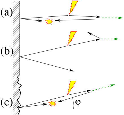
Figure 2: (Color on-line) Real-space representation of the scattering process responsible for the D-peak near graphene edges. The lightning represents the incoming photon which generates the electron-hole pair. The solid black arrows represent the quasi-classical trajectories of the electron and the hole. The dashed arrow represents the emitted phonon. The flash represents the radiative recombination of the electron-hole pair producing the scattered photon. (a) Backscattering off a translationally invariant edge is possible only at normal incidence (up to the quantum uncertainty). (b) For oblique incidence on a translationally invariant edge the reflection is specular, so the electron and the hole will not be able to meet at the same point. (c) For a rough edge backscattering is possible even at oblique incidence.

In the quasiclassical picture, the electron and the hole have to travel the same distance between creation and annihilation, as their velocities are equal. Then the process in Fig. 3 (a) has more phase space satisfying this restriction, and this process gives the main contribution to the Raman matrix element. This will be also shown by an explicit estimate in Sec. VI.2. Note that the three processes shown in Fig. 3, can be considered in the momentum space, as shown in Fig. 4. According to the abovesaid, the processes (b) and (c), often shown in the literature as an illustration of the double resonance,ThomsenReich2000 are in fact weaker than the process (a) by a factor $\sim\omega_{\mathrm{ph}}/\omega_{in}$.

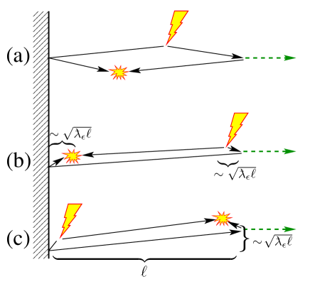
Figure 3: (Color on-line.) Real space representation of different contributions to the matrix element of the scattering process responsible for the D-peak at an ideal armchair edge, placed at $x=0$. The solid black arrows represent the quasi-classical trajectories of the electron and the hole corresponding to the three Green’s functions in Eqs. (32c), (32d). Trajectories (a), (b), (c) correspond to decomposition of each of the three Green’s functions in Eq. (32c). $\ell$ is the overall spatial extent of the process, and $\lambdabar_{\epsilon}=v/\epsilon$ is the electron wavelength divided by 2$\pi$.

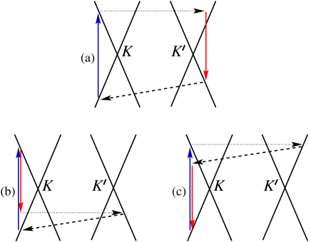
Figure 4: (Color on-line.) Momentum space representation of different contributions to the matrix element of the scattering process responsible for the D-peak at an armchair graphene edge, corresponding to the real space picture shown in Fig. 3. Solid lines represent the Dirac cones around $K$ and $K^{\prime}$ points of the first Brillouin zone. Vertical solid arrows represent interband electronic transitions accompanied by photon absorption or emission (photon wave vector is neglected), dashed arrows represent phonon emission, the horisontal dotted arrow represents the scattering from the edge.

II.3 Polarization dependence

The backscattering condition has immediate consequences for the polarization dependence of the Raman scattering intensity. Indeed, the matrix element of creation/annihilation of an electron and a hole pair with momenta ${\rm\bf p},-{\rm\bf p}$ (counted from the Dirac point) by a photon with the polarization ${\rm\bf e}$, is proportional to $[{\rm\bf e}\times{\rm\bf p}]_{z}$, reaching its maximum when ${\rm\bf e}\perp{\rm\bf p}$. Since a perfect edge conserves the component of momentum along the edge, the backscattering is possible only at normal incidence, as seen from Fig. 2).singularity This gives the polarization dependence of the D peak intensity as $I_{D}\propto\sin^{2}\varphi_{in}\sin^{2}\varphi_{out}$, where $\varphi_{in}$ and $\varphi_{out}$ are the angles between the polarizations of the incident and scattered photons and the normal to the edge. If one does not use the analyzer to fix the polarization of the scattered photons, the dependence is $I_{D}\propto\sin^{2}\varphi_{in}$. In experiments, however, the intensity never goes exactly to zero for the polarizations perpendicular to the edge, but remains a finite fraction $\varepsilon$ of the intensity in the maximum.Cancado2004 ; Gupta2009 ; Casiraghi2009 What determines this residual intensity in the minimum?

For an ideal edge the finite value of the intensity in the minimum is entirely due to the quantum uncertainty. Namely, the momenta of the electron and the hole upon their creation are not exactly opposite, but up to an uncertainty $\sim{1}/\delta{l}$; the annihilation occurs not exactly at the same spatial point, but within the spatial uncertainty $\delta{l}$. If the spatial extent of the process is $\ell$, the uncertaintly is estimated as $\delta{l}\sim\sqrt{\lambdabar_{\epsilon}\ell}$, and the ratio $\varepsilon$ of the intensities in the minimum and in the maximum (i. e., for polarizations perpendicular and parallel to the edge, respectively) should be small as a power of the small parameter quasiclassical parameter $\lambdabar_{\epsilon}/\ell$. The calculation is performed in Sec. VI.2, the result is given by Eqs. (42b) and (42c) for the detection without and with the analyzer, respectively. Up to logaritmic factors, the ratio $\varepsilon\sim\omega_{\mathrm{ph}}^{2}/\omega_{in}^{2}\sim(\lambdabar_{\epsilon}/\ell_{\mathrm{ph}})^{2}$. This corresponds to $\ell_{\mathrm{ph}}\sim\ell$, in accordance with the energy-time uncertainty principle, as discussed in the previous subsection.

For rough edges the intensity in the minimum is determined by the ability of the edge to backscatter electrons at oblique incidence, as shown in Fig. 2(c). If the edge is rough at the atomic scale, oblique backscattering is nearly as efficient as normal backscattering. Still, such oblique trajectories are longer than those corresponding to the normal incidence, so they are expected to have a smaller weight since the virtual electron-hole pair lives only for a restricted time. So one still can expect a minimum of intensity for perpendicular polarization, but it is of a purely geometrical origin, so one does not expect a parametric smallness of the ratio $\varepsilon$. The calculation using the model Sec. IV.2 for an atomically rough, is performed in Sec. VII.1, and the result is given by Eqs. (53b) and (LABEL:IDdisordc=) for the detection without and with the analyzer, respectively. In the former case the ratio $\varepsilon=1/3$, and the minimum is indeed for the polarization of the incident light perpendicular to the edge. With the analyzer, the absolute minimum is $\varepsilon={1}/10$, reached when the polarizer and the analyzer are oriented at the angle $\pi/3$ with respect to the edge and to each other. When the polarizer and the analyzer are both rotated parallel to each other, the minimum is $\varepsilon=1/5$.

For an edge consisiting of segments longer than electronic wavelength, $d_{e}\gg\lambdabar_{\epsilon}$, we first analyze the contribution of a single armchair segment. It is calculated in Sec. VIII, and given by Eqs. (LABEL:IDfragma=) and (LABEL:IDfragmb=) for the detection without and with the analyzer, respectively. The minimum is reached for the polarization, perpendicular to the armchair direction (which does not have to coincide with the average direction of the edge!), and is determined by the quantum diffraction of the electron on the segment, $\varepsilon\sim\lambdabar_{\epsilon}/d_{e}$ (provided that $\lambdabar_{\epsilon}/d_{e}\gtrsim\omega_{\mathrm{ph}}^{2}/\omega_{in}^{2}$, the ratio for the infinite armchair edge, which is the case when $d_{e}\lesssim{50}\>\mbox{nm}$ for $\omega_{in}=2\>\mbox{eV}$). To obtain contribution of the whole edge, it is sufficient to multiply these expression by the total number of such segments and replace $d_{e}$ by its average, provided that all armchair segments have the same orientation.

It is crucial, however, that up to three different orientations of armchair segments are possible, at the angle $\pi/3$ to each other. When contributions corresponding to several different orientations are added together, the polarization dependence may change quite dramatically, as was briefly discussed by the author and coworkers in Ref. Casiraghi2009, and is considered in more detail in Sec. VIII. Note that if the average direction of the edge is armchair or zigzag, the possible orientations of armchair segments are symmetric with respect to the average direction: three orientetaions at angles 0 and $\pm\pi/3$ for an armchair edge, and two at angles $\pm\pi/6$ for a zigzag edge. Most likely, the number of segments corresponding to “$+$” and “$-$” signs will be equal on the average. Then, by symmetry, the maximum of intensity in both cases will be reached for the polarization along the average direction of the edge, in agreement with recent experimental observations.Gupta2009 ; Casiraghi2009

When the average direction is armchair, the ratio between the minimum and the maximum of intensity is determined by the relative fraction of segments oriented at $\pm\pi/3$ with respect to those oriented along the average direction. When the average direction is zigzag, the polarization dependence is fully determined by the symmetry (on the average) between the two armchair directions, and is given by Eq. (LABEL:IDzigzag=). The ratio between the minimum and the maximum is $\varepsilon=1/3$ for detection without analyzer, and $\varepsilon=1/9$ for detection with an analyzer parallel to the polarizer of the incident light, again, in agreement with Refs. Gupta2009, ; Casiraghi2009, . Thus, quantum diffraction effects appear to be masked by the purely geometrical effects.

Remarkably, the quantum diffraction limit is still accessible if only two orientations of armchair segments are present (which is the case when the average direction is zigzag or close to it). It is sufficient to put the polarizer perpendicular to one of the armchair directions, and the analyzer perpendicular to the other one, thereby killing the leading specular contribution for both segments. In this polarization configuration the absolute minimum of the intensity is reached, and it is indeed determined by the quantum diffraction, as given by Eq. (66a).

II.4 Excitation position dependence

In Ref. Novotny, , confocal Raman spectroscopy was suggested and used as a way to probe the length scale $\ell$ which restricts the $D$ peak to be in the vicinity of the edge (the spatial extent of the Raman process). The idea is to focus the incident light beam as tightly as possible, so that its electric field $\mathcal{E}_{in}({\rm\bf r})$ has the shape $\mathcal{E}_{in}({\rm\bf r})\propto{e}^{-|{\rm\bf r}-{\rm\bf r}_{0}|^{2}/(2L^{2})}$, where the width $L$ can be measured independently, and the spot center position ${\rm\bf r}_{0}$ can be varied experimentally. Then, given that the intensity of the $D$ peak is proportional to

$$I_{D}\propto\int\mathcal{K}({\rm\bf r},{\rm\bf r}^{\prime})\,\mathcal{E}_{in}({\rm\bf r})\,\mathcal{E}_{in}^{*}({\rm\bf r}^{\prime})\,d^{2}{\rm\bf r}\,d^{2}{\rm\bf r}^{\prime},$$ (2)

where $\mathcal{K}({\rm\bf r},{\rm\bf r}^{\prime})$ is a certain kernel, decaying away from the edge with a characteristic length scale $\ell$, a measurement of the dependence $I_{D}({\rm\bf r}_{0})$ would give information on the kernel. The measurement would be especialy simple in the case $L\ll\ell$. In reality, however, the relation is the opposite: in Ref. Novotny, $L=186.5\>\mbox{nm}$, and $\ell$ is a few tens of nanometers at most.citeGupta

In this situation the dependence of the Raman intensity $I_{D}({\rm\bf r}_{0})$ is very close to the excitation intensity profile $|\mathcal{E}_{in}({\rm\bf r})|^{2}$, and the nonlocality of the kernel $\mathcal{K}({\rm\bf r},{\rm\bf r}^{\prime})$ manifests itself only in a slight change of shape of$I_{D}({\rm\bf r}_{0})$ with respect to $|\mathcal{E}_{in}({\rm\bf r})|^{2}$. In the first approximation it can be viewed just as small shift and broadening. When the signal-to-noise ratio is not sufficiently high to perform the full functional deconvolution, one has to assume a specific functional form for the kernel and do a few-parameter fit. It is clear that different functional forms will give values of $\ell$, differing by a factor of the order of 1. In Ref. Novotny, the form $\mathcal{K}({\rm\bf r},{\rm\bf r}^{\prime})=\theta(x)\,\theta(x^{\prime})\,e^{-2\gamma(x+x^{\prime})/\ell_{\gamma}}$ was assumed, where $x$ is the distance from the edge, $\theta(x)$ is the step function, and $\ell_{\gamma}=v/(2\gamma)$ is the electron inelastic scattering length [$2\gamma$ is the electron inelastic scattering rate, see Eq. (1)]. This assumption seems to contradict the fact that the lifetime of the virtual electron-hole pair is $\sim{1}/\omega_{\mathrm{ph}}$, discussed in Sec. II.2, as it was pointed out in Refs. megapaper, ; Casiraghi2009, .

The explicit form of the kernel $\mathcal{K}({\rm\bf r},{\rm\bf r}^{\prime})$ for an ideal armchair edge is calculated in Sec. VI.3, it is given by Eq. (44c), and it turns out to be more complicated than a simple exponential. In fact, it depends on both length scales, $\ell_{\mathrm{ph}}$ and $\ell_{\gamma}$. The length $\ell_{\mathrm{ph}}$ is shorter, but the spatial cutoff it provides is only power-law. The longer length $\ell_{\gamma}$ is responsible for the strong exponential cutoff. Which of the two lengths plays the dominant role in the Raman process, turns out to depend on the specific observable to be measured. The total integrated intensity for $\mathcal{E}_{in}({\rm\bf r})=\mathrm{const}$ is proportional to the integral $\int\mathcal{K}({\rm\bf r},{\rm\bf r}^{\prime})\,d^{2}{\rm\bf r}\,d^{2}{\rm\bf r}^{\prime}$, which is determined mainly by $\ell_{\mathrm{ph}}$, while $\ell_{\gamma}$ enters only in a logarithmic factor. The same can be said about the polarization dependence and diffraction corrections, discussed in the previous subsection. However, the change in the shape of $I_{D}({\rm\bf r}_{0})$, compared to the excitation intensity profile $|\mathcal{E}_{in}({\rm\bf r})|^{2}$, is determined by the second and higher moments of the kernel, $\int{x}^{n}(x^{\prime})^{n^{\prime}}\,\mathcal{K}({\rm\bf r},{\rm\bf r}^{\prime})\,d^{2}{\rm\bf r}\,d^{2}{\rm\bf r}^{\prime}$, with $n+n^{\prime}\geq{2}$. These moments turn out to be determined by the longer scale $\ell_{\gamma}$. Thus, the interpretation by the authors of Ref. Novotny, of their experiment is qualitatively correct.

Analysis of the experimental data of Ref. Novotny, using kernel (44c) gives $\ell_{\gamma}=66\>\mbox{nm}$, corresponding to $2\gamma\approx{11}\>\mbox{meV}$. Analogous analysis was done for the case of strongly disordered edge in Sec. VII.2, and in this model one obtains $\ell_{\gamma}=120\>\mbox{nm}$. Indeed, as the disordered edge gives more weight to oblique trajectories, as shown in Fig. 2(c), the effective distance from the edge at which the kernel decays, is shorter than for the normal incidence, so a larger value of $\ell_{\gamma}$ is required to fit the data.

The inelastic scattering rate for an electron with the energy $\epsilon$ due to phonon emission can be written as $2\gamma=(\lambda_{\Gamma}+\lambda_{K})\epsilon/2$,shortraman ; megapaper where $\lambda_{\Gamma}$ and $\lambda_{K}$ are dimensionless electron-phonon coupling constants [$\lambda_{K}$ is defined in Eq. (30), and $\lambda_{\Gamma}$ is defined analogously, but the optical phonons at the $\Gamma$ point should be considered]. The value of the constant $\lambda_{\Gamma}$ can be reliably taken to be about $\lambda_{\Gamma}\approx{0}.03$. Indeed, a DFT calculationPiscanec2004 gives $\lambda_{\Gamma}\approx{0}.028$; measurements of the dependence of the $G$-peak frequency $\omega_{G}$ on the electronic Fermi energy $\epsilon_{F}$, $d\omega_{G}/d|\epsilon_{F}|\approx\lambda_{\Gamma}/2\pi$ give $\lambda_{\Gamma}\approx{0}.034$Yan2007 and $\lambda_{\Gamma}\approx{0}.027$;Pisana2007 the value of $\lambda_{\Gamma}$ is not renormalized by the Coulomb interaction.BaskoAleiner The value of $\lambda_{K}$ has been debated recently.Calandra2007 ; BaskoAleiner ; Lazzeri2008 The measurements of the phonon group velocity (see Ref. Lazzeri2008, for the summary of the experimental data) give $\lambda_{K}\approx{0}.04$. The ratio between the two coupling constants can be also extracted from the experimental ratio of the two-phonon peak intensities,megapaper $2(\lambda_{K}/\lambda_{\Gamma})^{2}\approx{20}$,Ferrari2006 which gives $\lambda_{K}\approx{0}.10$.

Thus, $\lambda_{\Gamma}+\lambda_{K}\approx{0}.1\pm{0.03}$, seems to be a reasonable estimate. This estimate gives $2\gamma\approx{50}\>\mbox{meV}$ for electrons with the energy $\omega_{in}/2=0.98\>\mbox{eV}$, which translates into a value of $\ell_{\gamma}$ several times shorter than that following from the results of Ref. Novotny, .

II.5 On the Tuinstra-König relation

For a sample of a finite size $L_{a}$ the total $D$ peak intensity is proportional to the total length of the edge, i. e., the sample perimeter, so that $I_{D}\propto{L}_{a}$. At the same time, the intensity of the $G$ peak at 1581 cm^-1 is propotional to the area of the sample, i. e., $I_{G}\propto{L}_{a}^{2}$. These simple facts result in the so-called Tuinstra-König relation, established in experiments on graphite nanocrystallites long ago,Tuinstra1970 ; Knight1989 and confirmed experimentally many times afterwards:Dresselhaus1999 ; Cancado2006 ; Cancado2007 ; Sato2006 $I_{D}/I_{G}\propto{1}/L_{a}$. The proportionality coefficient cannot be determined universally; it clearly depends on the character of the edge (as an extreme case, one can imagine a hexagonal flake with entirely zigzag edges which do not give any $D$ peak at all, except at the junctions between them; then $I_{D}$ is not even proportional to $L_{a}$).

What is the boundary of validity of the Tuinstra-König relation on the small-size side? At the same time, it was noted in Ref. Ferrari2000, that since the atomic dispacement pattern corresponding to the $D$ peak must involve at least one aromatic ring, the size of the ring, a few angstroms, represents an absolute lower bound. From the results of the present work it follows that the dependence $I_{D}\propto{L}_{a}$ becomes logarithmically sensitive to the presence of the opposite edge, $I_{D}\propto{L}_{a}\ln(\omega_{\mathrm{ph}}{L}_{a}/v)$ if the size is smaller the electron inelastic length $L_{a}<v/(2\gamma)$, and the whole approach becomes invalid when $L_{a}\sim{v}/\omega_{\mathrm{ph}}\approx{4}\>\mbox{nm}$. The breakdown of the $1/L_{a}$ dependence has indeed been observed for $L_{a}$ smaller than a few nanometers.Zickler2006

III Free Dirac electrons

Figure 5: Honeycomb lattice with the $A$ and $B$ sublattices and the elementarty translation vectors.

$C_{6v}$	$E$	$C_{2}$	$2C_{3}$	$2C_{6}$	$\sigma_{a,b,c}$	$\sigma_{a,b,c}^{\prime}$
$A_{1}$	1	1	1	1	1	1
$A_{2}$	1	1	1	1	$-1$	$-1$
$B_{2}$	1	$-1$	1	$-1$	$1$	$-1$
$B_{1}$	1	$-1$	1	$-1$	$-1$	$1$
$E_{1}$	2	$-2$	$-1$	$1$	0	0
$E_{2}$	2	2	$-1$	$-1$	0	0

Table 1: Irreducible representations of the group $C_{6v}$ and their characters.

irrep	$A_{1}$	$B_{1}$	$A_{2}$	$B_{2}$	$E_{1}$	$E_{2}$
valley-diagonal matrices
matrix	$\openone$	$\Lambda_{z}$	$\Sigma_{z}$	$\Lambda_{z}\Sigma_{z}$	$\Sigma_{x},\,\Sigma_{y}$	$-\Lambda_{z}\Sigma_{y},\Lambda_{z}\Sigma_{x}$
valley-off-diagonal matrices
matrix	$\Lambda_{x}\Sigma_{z}$	$\Lambda_{y}\Sigma_{z}$	$\Lambda_{x}$	$\Lambda_{y}$	$\Lambda_{x}\Sigma_{y},-\Lambda_{x}\Sigma_{x}$	$\Lambda_{y}\Sigma_{x},\Lambda_{y}\Sigma_{y}$

Table 2: Classification of $4\times{4}$ hermitian matrices according to irreducible representations (irreps) of the $C_{6v}$ group.

In this section we summarize the model for the bulk graphene only, which is fully analogous to that of Ref. megapaper, . Properties of the edge are discussed in the next section.

We measure the single-electron energy $\epsilon$ from the Fermi level of the undoped (half-filled) graphene. The Fermi surface of undoped graphene consists of two points, called $K$ and $K^{\prime}$. Graphene unit cell contains two atoms, labeled $A$ and $B$ (see Fig. 5), each of them has one $\pi$-orbital, so there are two electronic states for each point of the first Brillouin zone (we disregard the electron spin). Thus, there are exactly four electronic states with zero energy. An arbitrary linear combination of them is represented by a 4-component column vector $\psi$. States with low energy are obtained by including a smooth position dependence $\psi({\rm\bf r})$, ${\rm\bf r}\equiv(x,y)$. The low-energy hamiltonian has the Dirac form:

$$\hat{H}_{0}=\int{d}^{2}{\rm\bf r}\,\hat{\psi}^{\dagger}({\rm\bf r})\,(-iv{\rm\bf\Sigma}\cdot{\rm\bf\nabla})\,\hat{\psi}({\rm\bf r}).$$ (3)

Here we used the second-quantized notation and introduced the electronic $\psi$-operators $\hat{\psi}({\rm\bf r}),\hat{\psi}^{\dagger}({\rm\bf r})$.

It is convenient to define the $4\times{4}$ isospin matrices ${\rm\bf\Sigma}\equiv(\Sigma_{x},\Sigma_{y})$, not through their explicit form, which depends on the choice of the basis (specific arrangement of the components in the column $\psi$), but through their transformation properties. Namely, all 16 generators of the $SU(4)$ group, forming the basis in the space of $4\times{4}$ hermitian matrices, can be classified according to the irreducible representations of $C_{6v}$, the point group of the graphene crystal (Tables 1 and 2). They can be represented as products of two mutually commuting algebras of Pauli matrices $\Sigma_{x},\Sigma_{y},\Sigma_{z}$ and $\Lambda_{x},\Lambda_{y},\Lambda_{z}$,McCann2006 ; AleinerEfetov which fixes their algebraic relations. By definition, $\Sigma_{x},\Sigma_{y}$ are the matrices, diagonal in the $K,K^{\prime}$ subspace, and transforming according to the $E_{1}$ representation of $C_{6v}$.

In the following we will take advantage of the symmetry with respect to time reversal. The action of the time-reversal operation on the four-component envelope function $\psi({\rm\bf r})$ is defined as

$$\psi({\rm\bf r})\mapsto U_{t}\psi^{*}({\rm\bf r}),$$ (4)

where $U_{t}$ is a unitary $4\times{4}$ matrix. when applied twice, the time reversal operation should give an identity, which results in an additional requirement $U_{t}U_{t}^{*}=\openone$. The explicit form of $U_{t}$ depends on the choice of the basis.

In those rare cases when a specific representation has to be chosen, we use that of Ref. AleinerEfetov, ,

$$\psi=\left[\begin{array}[]{c}\psi_{AK}\\ \psi_{BK}\\ \psi_{BK^{\prime}}\\ -\psi_{AK^{\prime}}\end{array}\right],$$ (5)

where the first subscript labels the sublattice ($A,B$), and the second one labels the valley ($K,K^{\prime}$). In this basis $\Sigma_{i}$ are the Pauli matrices acting within upper and lower 2-blocks of the column (the sublattice subspace), while $\Lambda_{i}$ are the Pauli matrices acting in the “external” subspace of the 2-blocks (the valley subspace). The time reversal matrix in this representation is given by $U_{t}=\Sigma_{y}\Lambda_{y}$.

The electron Green’s function, corresponding to the hamiltonian (3), is given by

$$G_{0}({\rm\bf p},\epsilon)=\frac{\epsilon+v{\rm\bf p}\cdot{\rm\bf\Sigma}}{\epsilon^{2}-(vp-i\gamma_{\epsilon})^{2}},$$ (6)

where ${\rm\bf p}$ and $\epsilon$ are electronic momentum and energy, counted from the Dirac point. The inelastic broadening $\gamma_{\epsilon}\ll|\epsilon|$ is introduced phenomenologically. In the coordinate representation the Green’s function is given by

$$G_{0}({\rm\bf r},\epsilon) = \frac{\epsilon+i\gamma_{\epsilon}\mathop{\mathrm{sgn}}\epsilon-iv{\rm\bf\Sigma}\cdot{\rm\bf\nabla}}{4iv^{2}}\,H_{0}^{(1)}(\zeta),$$ (7)

where $H_{0}^{(1)}(\zeta)$ is the Hankel function and $\zeta\equiv(|\epsilon|+i\gamma_{\epsilon})r/v$. We will mostly need the asymptotic form valid at distances $r\gg|\epsilon|/v$,

$$G_{0}({\rm\bf r},\epsilon)=-\sqrt{\frac{i\zeta}{2\pi}}\,\frac{e^{i\zeta}}{vr}\left[\frac{\mathop{\mathrm{sgn}}\epsilon+{\rm\bf\Sigma}\cdot{\rm\bf r}/r}{2}\left(1+\frac{i}{8\zeta}\right)\right.$$

$$-\left.\frac{\mathop{\mathrm{sgn}}\epsilon-{\rm\bf\Sigma}\cdot{\rm\bf r}/r}{2}\,\frac{i}{4\zeta}+O(\zeta^{-2})\right].$$ (8)

Any wave function $\psi({\rm\bf r})$ satisfying the Dirac equation, $(\epsilon+i\gamma_{\epsilon}\mathop{\mathrm{sgn}}\epsilon+iv{\rm\bf\Sigma}\cdot{\rm\bf\nabla})\psi({\rm\bf r})=0$, in some region $\mathcal{O}$ of space, satisfies also the Huygens-Fresnel principle. Namely, the value of $\psi({\rm\bf r})$ at an arbitrary point ${\rm\bf r}\in\mathcal{O}$ can be written as an integral over the boundary $\partial\mathcal{O}$,

$$\psi({\rm\bf r})=iv\oint\limits_{\partial\mathcal{O}}{\rm\bf n}\cdot\left[G_{0}({\rm\bf r}-{\rm\bf r}_{e},\epsilon)\,{\rm\bf\Sigma}\,\psi({\rm\bf r}_{e})\right]d{\rm\bf r}_{e}.$$ (9)

Here ${\rm\bf r}_{e}$ is the distance along the boundary, ${\rm\bf n}$ is the inner normal to the boundary. This relation follows from the Gauss theorem and the fact that $(p^{2}+\nabla^{2})H_{0}^{(1)}(pr)=4i\delta({\rm\bf r})$ for any $p$.

IV Models for electrons near the edge

IV.1 Translationally invariant edge

The main assumption of this subsection is that the component of the electronic momentum ${\rm\bf p}$ along the edge is conserved upon reflection, so that a plane wave is reflected as a plane wave. The most studied ideal zigzag and armchair edges fall into this category. Here we do not restrict ourselves just to zigzag or armchair edges, requiring only that the spatial period $d_{e}$ of the edge is smaller than half the electron wavelength, $d_{e}<\pi\lambdabar_{\epsilon}$. For $d_{e}\ll\lambdabar_{\epsilon}$ the reflection of electrons from the edge can be described by an effective boundary condition for the electronic wave function.McCann2004 ; Akhmerov2008

The edge is assumed to be a straight line determined by its normal unit vector ${\rm\bf n}$, so that graphene occupies the half-plane ${\rm\bf n}\cdot{\rm\bf r}>0$. The microscopic Schrödinger equation determines the effective boundary condition on the wave function $\psi({\rm\bf r})$, which for smooth functions (on the scale $d_{e}$) can be simply written as $\left.B\psi\right|_{\mathrm{edge}}=0$, where $B$ is a $4\times{4}$ hermitian matrix. The rank of $B$ is equal to 2 since the linear space of incident states at fixed energy is two-dimensional due to the valley degeneracy. Thus, it has two zero eigenvalues, while the other two can be set to 1 without the loss of generality (only the zero subspace of $B$ matters). Thus, one can impose the condition $B^{2}=B$. Equivalently, one can write $B=(\openone-M)/2$, where $M$ has the same eigenvectors as $B$, but its eigenvalues are equal to $\pm{1}$, hence $M^{2}=\openone$. To ensure current conservation, the condition $\left.B\psi\right|_{\mathrm{edge}}=0$ must automatically yield $\psi^{\dagger}({\rm\bf n}\cdot{\rm\bf\Sigma})\psi=0$; this means that $M({\rm\bf n}\cdot{\rm\bf\Sigma})+({\rm\bf n}\cdot{\rm\bf\Sigma})M=0$. Finally, the time reversal symmetry requires that the conditions $B\psi=0$ and $BU_{t}\psi^{*}=0$ must be equivalent, which yields $M^{*}=U_{t}^{\dagger}{M}U_{t}$. To summarize all the above arguments, the general energy-independent boundary condition has the form

$$\left.(\openone-M)\psi\right|_{\mathrm{edge}}=0,$$ (10)

where the $4\times{4}$ hermitian matrix $M$ satisfies the following conditions, which result to be the same as obtained in Ref. McCann2004, :

$$M^{2}=\openone,\quad M({\rm\bf n}\cdot{\rm\bf\Sigma})+({\rm\bf n}\cdot{\rm\bf\Sigma})M=0,\quad M=U_{t}M^{*}U_{t}^{\dagger}.$$ (11)

Matrices satisfying these constraints can be parametrized by an angle $\chi$ and a three-dimensional unit vector $(m_{x},m_{y},m_{z})$:Akhmerov2008

$$M = \left(\Sigma_{z}\cos\chi+[{\rm\bf n}\times{\rm\bf\Sigma}]_{z}\sin\chi\right)M_{\Lambda},$$ (12a)

$$M_{\Lambda} = \sum_{i=x,y,z}m_{i}\Lambda_{i},\;\;\;m_{i}\in\mathbb{R},\;\;\;\sum_{i=x,y,z}m_{i}^{2}=1.$$ (12b)

Without loss of generality we can assume $\cos\chi\geq{0}$ (the negative sign can always be incorporated in $M_{\Lambda}$).

Explicit expressions for the matrix $M$, corresponding to the edges shown in Fig. 1, can be obtained in the tight-binding model on the terminated honeycomb latticeBrey2006 [it is convenient to use representation (5)]. For the zigzag edge with ${\rm\bf n}=-{\rm\bf e}_{y}$ [Fig. 1(a)] the boundary condition is $\psi_{BK}=\psi_{BK^{\prime}}=0$, which gives $M=\Sigma_{z}\Lambda_{z}$. This agrees with the prediction of Ref. Cancado2004, that upon reflection from a zigzag edge the electron cannot scatter between the valleys, which corresponds to a valley-diagonal matrix $M$. For the armchair edge with ${\rm\bf n}={\rm\bf e}_{x}$ [Fig. 1(a) rotated by $2\pi/3$ counterclockwise] we have $\psi_{AK}+\psi_{AK^{\prime}}=\psi_{BK}+\psi_{BK^{\prime}}=0$, and $M=-\Sigma_{y}\Lambda_{y}$. It can be shown that in the nearest-neigbor tight-binding model on a terminated honeycomb lattice only zigzag and armchair boundary conditions can be obtained, the latter occurring only if the edge direction is armchair, while to obtain the full form of Eq. (12a), one has to include an on-site potential in the vicinity of the edge.Akhmerov2008

It is known for quite some time that a perfect zigzag edge supports states, confined to the edge.Stein1987 ; Tanaka1987 ; Fujita1996-1 ; Fujita1996-2 ; Dresselhaus1996 Let us see what class of boundary conditions is compatible with existence of such states. The wave function of an edge state must have the form

$$\psi({\rm\bf r})=\psi_{0}e^{-\kappa({\rm\bf n}\cdot{\rm\bf r})+ip_{\|}[{\rm\bf n}\times{\rm\bf r}]_{z}},\quad\kappa>0,$$ (13)

where the vector $\psi_{0}$ is such that the solution satisfies both the Dirac equation in the bulk with some energy $\epsilon$, as well as the boundary condition at the edge. It is convenient to make a unitary substitution $\psi_{0}=e^{i\Sigma_{x}\chi/2}e^{-i\Sigma_{z}\varphi_{\rm\bf n}/2}\tilde{\psi}_{0}$, where $\varphi_{\rm\bf n}$ is the polar angle of the direction ${\rm\bf n}$. Then the two conditions have the following form:

$$\left(i\kappa\Sigma_{x}+p_{\|}\cos\chi\Sigma_{y}+p_{\|}\sin\chi\Sigma_{z}\right)\tilde{\psi}_{0}=\frac{\epsilon}{v}\,\tilde{\psi}_{0},$$ (14a)

$$\Sigma_{z}M_{\Lambda}\tilde{\psi}_{0}=\tilde{\psi}_{0}.$$ (14b)

The boundary condition is satisfied by two linearly independent vectors $\tilde{\psi}_{\pm}$ which can be chosen to satisfy $\Sigma_{z}\tilde{\psi}_{\pm}=\pm\tilde{\psi}_{\pm}$ (to find them it is sufficient to diagonalize the matrix $M_{\Lambda}$). Each of them satisfies the first condition if and only if $\epsilon=\pm{v}p_{\|}\sin\chi$, $\kappa=\mp{p}_{\|}\cos\chi$. The requirement $\kappa>0$ leaves only one of them, $\tilde{\psi}_{-\mathop{\mathrm{sgn}}{p}_{\|}}$, and the energy of the edge state is $\epsilon=-v|p_{\|}|\sin\chi$. Thus, it seems that almost any edge can support a bound state, the exception being the case $\cos\chi=0$ (armchair-like edge), which thus seems to be a special rather than a general case.

Now we turn to the scattering (reflecting) states, which are the ones responsible for the edge-assisted Raman scattering. Even though the component $p_{\|}$ of the electron momentum ${\rm\bf p}$, parallel to the edge, is conserved, reflection can change the valley structure of the electron wave function. The general form of such solution is

$$\psi({\rm\bf r})=\psi_{\rm\bf p}e^{ip_{\perp}({\rm\bf n}\cdot{\rm\bf r})+ip_{\|}[{\rm\bf n}\times{\rm\bf r}]_{z}}+$$

$$\qquad{}+S_{\Lambda}[{\rm\bf n}\times{\rm\bf\Sigma}]_{z}\psi_{\rm\bf p}e^{-ip_{\perp}({\rm\bf n}\cdot{\rm\bf r})+ip_{\|}[{\rm\bf n}\times{\rm\bf r}]_{z}},$$ (15)

where $p_{\perp}=({\rm\bf n}\cdot{\rm\bf p})<0$, $p_{\|}=[{\rm\bf n}\times{\rm\bf p}]_{z}$, and $\psi_{\rm\bf p}$ is an eigenvector of $({\rm\bf p}\cdot{\rm\bf\Sigma})\psi_{\rm\bf p}=\pm|{\rm\bf p}|\psi_{\rm\bf p}$. The first term represents the wave incident on the edge, the second one is the reflected wave. The matrix $[{\rm\bf n}\times{\rm\bf\Sigma}]_{z}$ simply aligns the isospin of the reflected particle with the new direction of momentum. The unitary matrix $S_{\Lambda}$ represents a rotation in the valley subspace. It should be found from the boundary condition (10) (this is conveniently done in the basis of the eigenvectors of $M_{\Lambda}$), which gives

$$S_{\Lambda}=\zeta\,\frac{\Lambda_{0}+M_{\Lambda}(\cos\chi+\zeta^{*}\sin\chi)}{\Lambda_{0}+M_{\Lambda}(\cos\chi+\zeta\sin\chi)},$$ (16a)

$$\zeta=\pm\frac{1}{p}\left\{-[{\rm\bf n}\times{\rm\bf p}]_{z}+i({\rm\bf n}\cdot{\rm\bf p})\right\},\quad|\zeta|=1.$$ (16b)

For $\sin\chi=0$ (zigzag edge) we have $S_{\Lambda}=\zeta$. For $\cos\chi=0$ (armchair edge) we have $S_{\Lambda}=M_{\Lambda}$, independent of the direction of ${\rm\bf p}$. The reflected part of Eq. (15) can be identically rewritten using the Huygens-Fresnel principle, Eq. (9), as

$$\psi({\rm\bf r})=\psi_{\rm\bf p}e^{i{\rm\bf p}{\rm\bf r}}-\int\limits_{\mathrm{edge}}d{\rm\bf r}_{e}\,G_{0}({\rm\bf r}-{\rm\bf r}_{e},\epsilon)\,v\Sigma_{z}S_{\Lambda}\psi_{\rm\bf p}e^{i{\rm\bf p}{\rm\bf r}_{e}},$$ (17)

so that $-v\Sigma_{z}S_{\Lambda}$ can be viewed as the $T$-matix of the edge.

When $S_{\Lambda}$ does not depend on the direction of ${\rm\bf p}$ (armchair edge), it is easy to write down the exact explicit expression for the single-particle Green’s function:

$$G({\rm\bf r},{\rm\bf r}^{\prime};\epsilon) = G_{0}({\rm\bf r}-{\rm\bf r}^{\prime},\epsilon)$$

$${}+G_{0}({\rm\bf r}-{\rm\bf r}^{\prime}+2{\rm\bf n}({\rm\bf n}\cdot{\rm\bf r}^{\prime}),\epsilon)\,[{\rm\bf n}\times{\rm\bf\Sigma}]_{z}S_{\Lambda}.$$

The second term represents nothing but the contribution of a fictitious image source of particles, appropriately rotated, and placed at the point ${\rm\bf r}^{\prime}-2{\rm\bf n}({\rm\bf n}\cdot{\rm\bf r}^{\prime})$ obtained from ${\rm\bf r}^{\prime}$ by the reflection with respect to the edge. In the quasiclassical approximation (analogous to geometric optics), Eq. (LABEL:imagesource=) is also valid for a general edge at large distances $r,r^{\prime}\gg{v}/|\epsilon|$, provided that position-dependent $S_{\Lambda}$ is taken, determined by

$$\zeta=-\mathop{\mathrm{sgn}}\epsilon\,\frac{i({\rm\bf n}\cdot({\rm\bf r}+{\rm\bf r}^{\prime}))+[{\rm\bf n}\times({\rm\bf r}-{\rm\bf r}^{\prime})]_{z}}{\sqrt{({\rm\bf n}\cdot({\rm\bf r}+{\rm\bf r}^{\prime}))^{2}+[{\rm\bf n}\times({\rm\bf r}-{\rm\bf r}^{\prime})]_{z}^{2}}}.$$ (19)

Again, using the Huygens-Fresnel principle, we can rewrite Eq. (LABEL:imagesource=) identically as

$$G({\rm\bf r},{\rm\bf r}^{\prime};\epsilon)=G_{0}({\rm\bf r}-{\rm\bf r}^{\prime},\epsilon)$$

$$\qquad{}-\int\limits_{\mathrm{edge}}d{\rm\bf r}_{e}\,G_{0}({\rm\bf r}-{\rm\bf r}_{e},\epsilon)\,v\Sigma_{z}S_{\Lambda}\,G_{0}({\rm\bf r}_{e}-{\rm\bf r}^{\prime},\epsilon).$$

(20)

IV.2 Atomically rough edge

As discussed in Sec. II.1, when the edge is rough on the atomic length scale, electron scattering is random both in all directions and between the two valleys. This case will be of main interest for us, as it (i) represents the opposite limiting case to that of an ordered edge, and (ii) can be described by a simple model proposed below. The main assumption is that each point of an atomically rough edge acts as an independent point scatterer, independent from other segments. Associating thus a $T$-matrix to each point of the edge, we write the scattered wave function in the form

$$\psi({\rm\bf r})=\psi_{\rm\bf p}e^{i{\rm\bf p}{\rm\bf r}}$$

$$\qquad{}+\int\limits_{\mathrm{edge}}d{\rm\bf r}_{e}\,G_{0}({\rm\bf r}-{\rm\bf r}_{e},\epsilon)\,T({\rm\bf s},{\rm\bf e}_{\rm\bf p};{\rm\bf r}_{e})\,\psi_{\rm\bf p}e^{i{\rm\bf p}{\rm\bf r}_{e}},$$ (21)

$${\rm\bf s}=\frac{{\rm\bf r}-{\rm\bf r}_{e}}{|{\rm\bf r}-{\rm\bf r}_{e}|},\quad{\rm\bf e}_{\rm\bf p}=\frac{{\rm\bf p}}{|{\rm\bf p}|},$$

where energy argument of the Green’s function $\epsilon=\pm{v}p$ for electrons and holes, respectively. The (one-dimensional) integration is performed along the edge, which is assumed to be a straight line determined, as in the previous subsection, by the condition $({\rm\bf n}\cdot{\rm\bf r}_{e})=0$, where the unit vector ${\rm\bf n}$ is the normal to the edge. The unit vectors ${\rm\bf e}_{\rm\bf p}$ and ${\rm\bf s}$ indicate the incident and scattering directions.

The $T$-matrix must satisfy (i) the particle conservation condition (unitarity), and (ii) the time reversal symmetry (reciprocity),

$$T({\rm\bf s},{\rm\bf e}_{\rm\bf p};{\rm\bf r}_{e})=U_{t}\,T^{T}(-{\rm\bf e}_{\rm\bf p},-{\rm\bf s};{\rm\bf r}_{e})\,U_{t}^{\dagger}.$$ (22)

Here $T^{T}$ stands for the $4\times{4}$ matrix transpose. Unitarity and reciprocity are discussed in Appendix A in the context of a general scattering theory, similar to that for light scattering on a rough surface.Brown1984 We propose the following form of the $T$-matrix:

$$T(p{\rm\bf s},{\rm\bf p};{\rm\bf r}_{e})=-\sqrt{\rho({\rm\bf s},{\rm\bf e}_{\rm\bf p})}\,v\Sigma_{z}S_{\Lambda}({\rm\bf r}_{e}).$$ (23a)

The angular factor $$\rho({\rm\bf s},{\rm\bf e}_{\rm\bf p})$$ ensures the particle conservation (unitarity of the edge scattering, see Appendix A for details),

$$\rho({\rm\bf s},{\rm\bf e}_{\rm\bf p})=\frac{-2({\rm\bf n}\cdot{\rm\bf e}_{\rm\bf p})({\rm\bf n}\cdot{\rm\bf s})}{1-({\rm\bf n}\cdot{\rm\bf e}_{\rm\bf p})({\rm\bf n}\cdot{\rm\bf s})-[{\rm\bf n}\times{\rm\bf e}_{\rm\bf p}]_{z}[{\rm\bf n}\times{\rm\bf s}]_{z}}.$$ (23b)

If we introduce the angles of incidence and scattering by $$({\rm\bf n}\cdot{\rm\bf e}_{\rm\bf p})=-\cos\varphi_{i} ({\rm\bf n}\cdot{\rm\bf s})=\cos\varphi_{s} [{\rm\bf n}\times{\rm\bf e}_{\rm\bf p}]_{z}=\sin\varphi_{i} [{\rm\bf n}\times{\rm\bf s}]_{z}=\sin\varphi_{s} \varphi_{s}=\varphi_{i} \rho=2\cos\varphi_{i}\cos\varphi_{s}/[1+\cos(\varphi_{i}+\varphi_{s})] \Sigma T \Sigma_{z} i[{\rm\bf n}\times{\rm\bf\Sigma}]_{z}$$, , , , the specular direction corresponding to , then . Note that since the structure of the wave functions in the -subspace is fixed by the direction of momentum, one may suggest slightly different forms of Eq. (23b) which would be equivalent. For example, the -matrix obtained by from Eq. (23b) by replacement of by and by changing the sign of the third term in the denominator in Eq. (23b) would have the same matrix elements between Dirac eigenstates of the same energy.

For a coordinate-independent $S_{\Lambda}$ the ${\rm\bf r}_{e}$ integration eliminates all directions ${\rm\bf s}$ different from the specular one. Since for the latter $\rho=1$, Eq. (23a) reduces to Eq. (17). In this case $S_{\Lambda}$ can be identified with the scattering matrix. For the short-range disorder such identification is not possible, since scattering process is necessarily non-local on the length scale of at least $\sim{1}/p$. The connection between the $T$-matrix in Eq. (21) and the scattering matrix is more complicated, and is discuss in detail in Appendix A. Here we only mention that it would make absolutely no sense to require the unitarity of $S_{\Lambda}({\rm\bf r}_{e})$ at each given point. Instead, we use the following form:

$$S_{\Lambda}({\rm\bf r}_{e})=\varpi({\rm\bf r}_{e})\sum_{i=x,y,z}m_{i}({\rm\bf r}_{e})\,\Lambda_{i},\quad\sum_{i=x,y,z}m_{i}^{2}({\rm\bf r}_{e})=1.$$ (23c)

Here $\varpi({\rm\bf r}_{e})$ is a complex gaussian random variable whose real and imaginary parts are distributed independently and identically (so its phase is uniformly distributed between 0 and $2\pi$). The numbers $m_{x},m_{y},m_{z}$, which can be viewed as components of a unit three-dimensional vector, must be real to ensure the time-reversal symmetry. One may assume them to be constant or taking just few definite values, which would correspond the edge to be composed of segments with $a\ll{d}_{e}\lesssim{1}/p$ of definite types (e. g., zigzag or armchair). For $d_{e}\sim{a}$, when the scattering between the valleys is completely random, the vector $(m_{x},m_{y},m_{z})$ can be taken uniformly distributed over the unit sphere. We assume the matrices $S_{\Lambda}({\rm\bf r}_{e})$ to be uncorrelated at different points on the edge, distant by more than $d_{e}$, by writing

$$\overline{\varpi({\rm\bf r}_{e})\,\varpi^{*}({\rm\bf r}_{e}^{\prime})}=\frac{\pi{v}}{|\epsilon|}\,\delta({\rm\bf r}_{e}-{\rm\bf r}_{e}^{\prime}).$$ (23d)

Here the overline denotes the ensemble averaging. However, we assume that this product is self-averaging upon spatial integration, i. e., that Eq. (23d) holds even in the absence of the ensemble averaging when integrated over a sufficiently long segment of the edge (namely, longer than $d_{e}$). The prefactor $\pi{v}/|\epsilon|$ at the $\delta$-function ensures the unitarity of scattering, see Appendix A.

Eq. (21) for the wave function yields an analogous expression for the Green’s function, valid sufficiently far from the edge, $({\rm\bf n}\cdot{\rm\bf r})\gg{v}/|\epsilon|$, $({\rm\bf n}\cdot{\rm\bf r}^{\prime})\gg{v}/|\epsilon|$:

$$G({\rm\bf r},{\rm\bf r}^{\prime};\epsilon)=G_{0}({\rm\bf r}-{\rm\bf r}^{\prime},\epsilon)+$$

$$\qquad{}+\int\limits_{\mathrm{edge}}d{\rm\bf r}_{e}\,G_{0}({\rm\bf r}-{\rm\bf r}_{e},\epsilon)\,T({\rm\bf s},{\rm\bf s}^{\prime};{\rm\bf r}_{e})\,G_{0}({\rm\bf r}_{e}-{\rm\bf r}^{\prime},\epsilon),$$ (24)

$${\rm\bf s}=\frac{{\rm\bf r}-{\rm\bf r}_{e}}{|{\rm\bf r}-{\rm\bf r}_{e}|},\quad{\rm\bf s}^{\prime}=-\frac{{\rm\bf r}^{\prime}-{\rm\bf r}_{e}}{|{\rm\bf r}^{\prime}-{\rm\bf r}_{e}|}.$$ (25)

V Phonons and Raman scattering

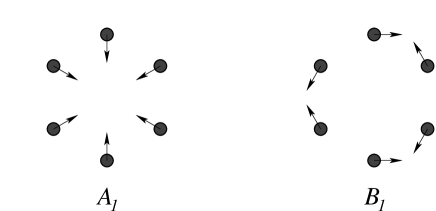
Figure 6: Phonon modes responsible for the Raman $D$ peak.

We restrict our attention to scalar phonons with wave vectors close to $K$ and $K^{\prime}$ points – those responsible for the Raman $D$ peak. The two real linear combinations of the modes at $K$ and $K^{\prime}$ points transform according to $A_{1}$ and $B_{1}$ representations of $C_{6v}$ and are shown in Fig. 6. We take the magnitude of the carbon atom displacement as the normal coordinate for each mode, denoted by $u_{a}$ and $u_{b}$, respectively. Upon quantization of the phonon field, the displacement operators $\hat{u}_{a},\hat{u}_{b}$ and the lattice hamiltonian $\hat{H}_{\mathrm{ph}}$ are expressed in terms of the phonon creation and annihilation operators $\hat{b}^{\dagger}_{{\rm\bf q}\mu},\hat{b}_{{\rm\bf q}\mu}$, $\mu=a,b$, as

$$\hat{u}_{\mu}({\rm\bf r})=L_{x}L_{y}\int\frac{d^{2}{\rm\bf q}}{(2\pi)^{2}}\frac{\hat{b}_{{\rm\bf q}\mu}e^{i{\rm\bf q}{\rm\bf r}}+\hat{b}_{{\rm\bf q}\mu}^{\dagger}e^{-i{\rm\bf q}{\rm\bf r}}}{\sqrt{2NM\omega_{\mathrm{ph}}}},$$ (26a)

$$\hat{H}_{\mathrm{ph}}=L_{x}L_{y}\int\frac{d^{2}{\rm\bf q}}{(2\pi)^{2}}\sum_{\mu=a,b}\omega_{\mathrm{ph}}\left(\hat{b}_{{\rm\bf q}\mu}^{\dagger}\hat{b}_{{\rm\bf q}\mu}+\frac{1}{2}\right).$$ (26b)

The crystal is assumed to have the area $L_{x}L_{y}$, and to contain $N$ carbon atoms of mass $M$. The area per carbon atom is $L_{x}L_{y}/N=\sqrt{27}a^{2}/4$.

The phonon frequency $\omega_{\mathrm{ph}}\approx{1350}\>\mbox{cm}^{-1}$, standing in Eq. (26b), is assumed to be independent of the phonon momentum. To check the validity of this assumption one should compare the corresponding energy scale (the spread of the phonon momenta $\Delta{q}$ multiplied by the phonon group velocity $v_{\mathrm{ph}}$) with the electronic energy uncertainty. The latter is given by $\omega_{\mathrm{ph}}$ itself. Recalling that phonon emission corresponds to the backscattering of the electron (hole), $\Delta{q}$ is given by the uncertainty of the electronic momentum, $\Delta{q}\sim\omega_{\mathrm{ph}}/v$. Since $v_{\mathrm{ph}}/v\approx{7}\cdot{10}^{-3}\ll{1}$, the phonon dispersion can be safely neglected.

If we neglect the phonon dispersion, the normal modes and the phonon hamiltonian can be rewritten in the coordinate representation by introducing the creation and annihilation operators for a phonon in a given point of the sample:

$$\hat{\Phi}_{\mu}({\rm\bf r})=\sum_{\rm\bf q}\frac{\hat{b}_{{\rm\bf q},\mu}e^{i{\rm\bf q}{\rm\bf r}}}{\sqrt{L_{x}L_{y}}},$$ (27a)

$$\hat{u}_{\mu}({\rm\bf r})=\sqrt{\frac{L_{x}L_{y}}{2NM\omega_{\mathrm{ph}}}}\left[\hat{\Phi}_{\mu}({\rm\bf r})+\hat{\Phi}_{\mu}^{\dagger}({\rm\bf r})\right],$$ (27b)

$$\hat{H}_{\mathrm{ph}}=\sum_{\mu}\omega_{\mathrm{ph}}\int{d}^{2}{\rm\bf r}\left[\hat{\Phi}_{\mu}({\rm\bf r})\hat{\Phi}_{\mu}^{\dagger}({\rm\bf r})+\frac{N}{2L_{x}L_{y}}\right].$$ (27c)

Then it is convenient to define the phonon Green’s function as the time-ordered average of the $\Phi$-operators,

$$D_{\mu}^{(+)}({\rm\bf r},\omega)=-i\int\langle\mathrm{T}\hat{\Phi}_{\mu}({\rm\bf r},t)\,\hat{\Phi}^{\dagger}_{\mu}({\rm\bf 0},0)\rangle e^{i\omega{t}}d^{2}{\rm\bf r}\,dt=$$

$$\qquad=\frac{\delta({\rm\bf r})}{\omega-\omega_{\mathrm{ph}}+io}.$$ (28)

By symmetry, in the electron-phonon interaction hamiltonian the normal mode displacements $u_{\mu}$ couple to the corresponding valley-off-diagonal $4\times{4}$ matrices from Table 2:megapaper

$$\hat{H}_{\mathrm{int}}=F_{K}\int{d}^{2}{\rm\bf r}\,\hat{\psi}^{\dagger}({\rm\bf r})\left[\hat{u}_{a}({\rm\bf r})\Lambda_{x}\Sigma_{z}+\hat{u}_{b}({\rm\bf r})\Lambda_{y}\Sigma_{z}\right]\hat{\psi}({\rm\bf r}).$$ (29)

Here $F_{K}$ is the coupling constant having the dimensionality of a force. It is more convenient to use the dimensionless coupling constant

$$\lambda_{K}=\frac{F_{K}^{2}}{M\omega_{\mathrm{ph}}v^{2}}\frac{\sqrt{27}a^{2}}{4}.$$ (30)

The value of $\lambda_{K}$ was discussed in Sec. II.4.

The hamiltonian describing interaction of electrons with light is obtained from the Dirac hamiltonian (3) by replacement ${\rm\bf\nabla}\to{\rm\bf\nabla}-i(e/c)\hat{{\rm\bf A}}$, where the vector potential $\hat{{\rm\bf A}}$ is expressed in terms of creation and annihilation operators $\hat{a}^{\dagger}_{{\rm\bf Q},\ell},\hat{a}_{{\rm\bf Q},\ell}$ of three-dimensional photons in the quantization volume $V=L_{x}L_{y}L_{z}$, labeled by the three-dimensional wave vector ${\rm\bf Q}$ and two transverse polarizations $\ell=1,2$ with unit vectors ${\rm\bf e}_{{\rm\bf Q},\ell}$:

$$\hat{{\rm\bf A}}({\rm\bf r})=\sum_{{\rm\bf Q},\ell}\sqrt{\frac{2\pi{c}}{VQ}}\left({\rm\bf e}_{{\rm\bf Q},\ell}\hat{a}_{{\rm\bf Q},\ell}e^{i{\rm\bf Q}{\rm\bf r}}+\mathrm{h.c.}\right).$$ (31)

The derivation of the formal expression for the Raman scattering probability is fully analogous to that given in Ref. megapaper, . The only difference is that the calculation is done in the coordinate representation. As a result, we obtain the following expression for the probability for an incident photon with wave vector ${\rm\bf Q}_{in}$ and polarization ${\rm\bf e}_{in}$ to be scattered with emission of a single phonon within an elementary area $d^{2}{\rm\bf R}$ around a given point ${\rm\bf R}$:

$$\frac{dI_{D}}{d^{2}{\rm\bf R}} = \frac{1}{cL_{x}L_{y}}\sum_{{\rm\bf e}_{out}}\int\frac{d^{3}{\rm\bf Q}_{out}}{(2\pi)^{3}}\,2\pi\delta(c|{\rm\bf Q}_{out}|-\omega_{out})$$ (32a)

$${}\times\sum_{\mu=a,b}|2\mathcal{M}_{\mu}|^{2},$$

$$\mathcal{M}_{\mu} = \sqrt{\frac{\lambda_{K}}{2}}\frac{2\pi{e}^{2}v^{3}}{\sqrt{\omega_{in}\omega_{out}}}\int\frac{d\epsilon}{2\pi}\,{d}^{2}{\rm\bf r}_{in}\,{d}^{2}{\rm\bf r}_{out}$$ (32b)

$${}\times e^{i{\rm\bf Q}_{in}{\rm\bf r}_{in}-i{\rm\bf Q}_{out}{\rm\bf r}_{out}}\mathop{\mathrm{Tr}}\left\{\mathcal{D}_{\mu}+\bar{\mathcal{D}}_{\mu}\right\},$$

$$\mathcal{D}_{a,b} = G({\rm\bf r}_{out},{\rm\bf r}_{in};\epsilon)({\rm\bf e}_{in}\cdot{\rm\bf\Sigma})\,G({\rm\bf r}_{in},{\rm\bf R};\epsilon-\omega_{in})\,$$ (32c)

$${}\times\Lambda_{x,y}\Sigma_{z}\,G({\rm\bf R},{\rm\bf r}_{out};\epsilon-\omega_{out})({\rm\bf e}_{out}^{*}\cdot{\rm\bf\Sigma}),$$

$$\bar{\mathcal{D}}_{a,b} = G({\rm\bf r}_{in},{\rm\bf r}_{out};\epsilon)\,({\rm\bf e}_{out}^{*}\cdot{\rm\bf\Sigma})\,G({\rm\bf r}_{out},{\rm\bf R};\epsilon+\omega_{out})\,$$ (32d)

$${}\times\Lambda_{x,y}\Sigma_{z}\,G({\rm\bf R},{\rm\bf r}_{in};\epsilon+\omega_{in})({\rm\bf e}_{in}\cdot{\rm\bf\Sigma}).$$

Here $G({\rm\bf r},{\rm\bf r}^{\prime};\epsilon)$ is the electronic Green’s function corresponding to the full single-particle part of the hamiltonian (i. e., including not only the Dirac term, but the edge as well). It can be represented in terms of the exact single-electron eigenfunctions $\psi_{s}({\rm\bf r})$ and energies $\epsilon_{s}$ as a sum over the eigenstates $s$:

$$G({\rm\bf r},{\rm\bf r}^{\prime};\epsilon)=\sum_{s}\frac{\psi_{s}({\rm\bf r})\,\psi^{\dagger}_{s}({\rm\bf r})}{\epsilon-\epsilon_{s}+i\gamma_{\epsilon}\mathop{\mathrm{sgn}}\epsilon}.$$ (33)

Using this representation, integrating over the energy and the coordinates one obtains Eq. (1). The summation in Eq. (32a) is performed over the wave vectors ${\rm\bf Q}_{out}$ and the polarizations ${\rm\bf e}_{out}$ of the scatered photon. When integrated over the area of the crystal, Eq. (32a) gives the absolute dimensionless probability of the one-phonon Raman scattering for a single incident photon.

The matrix element $\mathcal{M}_{\mu}$ can always be represented in the form

$$\mathcal{M}_{\mu}=\mathcal{M}_{\mu}^{x}(e_{out}^{x})^{*}+\mathcal{M}_{\mu}^{y}(e_{out}^{y})^{*}.$$ (34)

If one collects all the light scattered in the full solid angle $4\pi$, without analyzing the polarization, the integration over the angles of ${\rm\bf Q}_{out}$ is straightforward. It gives

$$\frac{dI_{D}}{d^{2}{\rm\bf R}}=\frac{8}{3\pi}\,\frac{\omega_{out}^{2}}{c^{4}L_{x}L_{y}}\,\sum_{\mu=a,b}\left(|\mathcal{M}_{\mu}^{x}|^{2}+|\mathcal{M}_{\mu}^{y}|^{2}\right).$$ (35a)

The dependence on the polarization of the scattered light is obtained most easily when the light is collected in a small solid angle $$o_{out}\ll{4\pi} \varphi_{out} x$$ around the normal (the case of an arbitrary solid angle was considered in Ref. megapaper, ). If the analyzer is oriented at an angle to the  axis, the polarization-dependent intensity is given by

$$\frac{dI_{D}}{d^{2}{\rm\bf R}}=\frac{o_{out}}{\pi^{2}}\frac{\omega_{out}^{2}}{c^{4}L_{x}L_{y}}\sum_{\mu=a,b}\left|\mathcal{M}_{\mu}^{x}\cos\varphi_{out}+\mathcal{M}_{\mu}^{y}\sin\varphi_{out}\right|^{2}.$$ (35b)

Eq. (31) corresponds to the free-space quantization of the electromagnetic field whose normal modes are plane waves. In the case of a spatially resolved experiment as in Ref. Novotny, , Eqs. (32a), (32b) in order to account for the spatial profile of the electric field, induced by the focusing lens. Namely, the electric field, corresponding to a single photon with a wave vector ${\rm\bf Q}_{in}$, incident from vacuum, should be replaced by the field $\mathcal{E}_{in}({\rm\bf r}_{in})$ of the focused laser beam,

$$i\sqrt{\frac{2\pi\omega_{in}}{L_{x}L_{y}L_{z}}}\,{\rm\bf e}_{in}e^{i{\rm\bf Q}_{in}{\rm\bf r}_{in}}\to{\rm\bf e}_{in}\mathcal{E}_{in}({\rm\bf r}_{in}).$$ (36)

As long as the distance between the lens and the sample is much larger than the light wavelegth, the summation over the continuum of the final states of the scattered photon can still be performed using the vacuum mode structure. Finally, dividing the resulting probability by the photon attempt period $L_{z}/c$, we obtain the number of photons emitted per unit time, $dI_{D}/dt$ (which is more appropriate when the incident light is characterized by its electric field strength). As a result, Eqs. (32a), (32b) are modified as follows:

$$\frac{dI_{D}}{d^{2}{\rm\bf R}\,dt} = \frac{1}{2\pi\omega_{in}}\sum_{{\rm\bf e}_{out}}\int\frac{d^{3}{\rm\bf Q}_{out}}{(2\pi)^{3}}\,2\pi\delta(c|{\rm\bf Q}_{out}|-\omega_{out})$$ (37a)

$${}\times\sum_{\mu=a,b}|2\mathcal{M}_{\mu}|^{2},$$

$$\mathcal{M}_{\mu} = \sqrt{\frac{\lambda_{K}}{2}}\frac{2\pi{e}^{2}v^{3}}{\sqrt{\omega_{in}\omega_{out}}}\int\frac{d\epsilon}{2\pi}\,{d}^{2}{\rm\bf r}_{in}\,{d}^{2}{\rm\bf r}_{out}$$ (37b)

$${}\times\mathcal{E}_{in}({\rm\bf r}_{in})\,e^{-i{\rm\bf Q}_{out}{\rm\bf r}_{out}}\mathop{\mathrm{Tr}}\left\{\mathcal{D}_{\mu}+\bar{\mathcal{D}}_{\mu}\right\}.$$

VI Raman scattering on a translationally invariant edge

VI.1 General considerations

For simplicity we consider an armchair edge characterized by ${\rm\bf n}={\rm\bf e}_{x}$, $M=-\Sigma_{y}\Lambda_{y}$, as discussed in the previous section. Due to the translational invariance in the $y$ direction, it is sufficient to calculate the probability of phonon emission at the point ${\rm\bf R}=X{\rm\bf e}_{x}$. As we will see below, the main contribution to the signal comes from $X\gg\lambdabar_{\epsilon}=2v/\omega_{in}$. In this regime the motion of the photoexcited electron-hole pair can be described quasiclassically, and the asymptotic large-distance expansion for the Green’s functions, Eq. (8), can be used. Namely, the electron and the hole can be viewed as wave packets of the size $\sim\sqrt{\lambdabar_{\epsilon}{X}}$, propagating across the crystal along classical trajectories. Initially, they are created in the same region of space of the size $\sim\sqrt{\lambdabar_{\epsilon}{X}}$ with opposite momenta and opposite velocities. As they undergo scattering processes (emission of a phonon or reflection from the edge), they change the directions of their momenta. In order to recombine radiatively and contribute to Raman signal, the electron and the hole should meet again within a spatial region of the size $\sim\sqrt{\lambdabar_{\epsilon}{X}}$. Clearly, these conditions can be fulfilled if all momenta are almost perpendicular to the edge. Small deviations by an angle $\sim\sqrt{\lambdabar_{\epsilon}/X}$ are allowed by quantum uncertainty. These considerations are illustrated by Fig. 3.

Emission of one of the phonons shown in Fig. 6 corresponds to intervalley scattering of the photoexcited electron or the hole, as represented formally by one of the valley-off-diagonal matrices $\Lambda_{x}$ or $\Lambda_{y}$ in the matrix element, see Eqs. (32b)–(32d). For the process to be allowed, another act of intervalley scattering is required, so one of the three electronic Green’s functions in Eqs. (32c), (32d) must contain another $\Lambda_{x}$ or $\Lambda_{y}$ matrix from the decomposition (LABEL:imagesource=). Otherwise, the trace in Eq. (32b) vanishes. Thus, for an armchair edge with $M=-\Lambda_{y}\Sigma_{y}$ only the $B_{1}$ phonon can be emitted, so $\mathcal{M}_{a}=0$, $\mathcal{M}_{b}=\mathcal{M}$. Trajectories, corresponding to decomposition of each of the three Green’s functions in Eq. (32c) are shown in Fig. 3 (a), (b), (c), respectively. According to the quasiclassical picture, the electron and the hole have to travel the same distance between creation and annihilation, as their velocities are equal. Then the process in Fig. 3 (a) has more phase space satisfying this restriction, and this process gives the main contribution to the Raman matrix element. This will be also shown explicitly below.

The general polarization structure of the matrix element, compatible with the reflection symmetry $y\to{-}y$ possessed by the armchair edge, is

$$\mathcal{M} = \mathcal{M}_{\|}e_{in}^{y}(e_{out}^{y})^{*}+\mathcal{M}_{\perp}e_{in}^{x}(e_{out}^{x})^{*}$$ (38)

$$= \mathcal{M}_{\|}\sin\varphi_{in}\sin\varphi_{out}+\mathcal{M}_{\perp}\cos\varphi_{in}\cos\varphi_{out}$$

(we introduced $\varphi_{in},\varphi_{out}$, the polar angles of the polarization vectors). Since the interband transition dipole moment is perpendicular to the electronic momentum, and for a regular edge the momentum is (almost) perpendincular to the edge, $\mathcal{M}_{\perp}$ is entirely due to quantum diffraction. Thus, $\mathcal{M}_{\perp}$ is smaller than $\mathcal{M}_{\|}$ by the parameter $\lambdabar_{\epsilon}/X\ll{1}$ (it is this parameter that governs the quantum diffraction, as discussed above). Nevertheless, in a polarization-resolved experiment the two intensities can be measured independently, so below we calculate both $\mathcal{M}_{\|}$ and $\mathcal{M}_{\perp}$, each to the leading order in $\lambdabar_{\epsilon}/X$.

VI.2 Spatially integrated intensity and polarization dependence

In this subsection the electric field of the excitation wave is assumed to be spatially homogeneous. As displacements along the edge are expected to be parametrically smaller than those away from the edge, $|y|\sim\sqrt{x\lambdabar_{\epsilon}}$, we use the paraxial approximation, $|{\rm\bf r}|\approx|x|+y^{2}/(2|x|)$. The Green’s function can be approximated as

$$G_{0}({\rm\bf r},\epsilon) \approx -\sqrt{\frac{i|\epsilon|}{2\pi{v}^{3}|x|}}\,e^{(i|\epsilon|-\gamma)|x|/v+i|\epsilon|y^{2}/(2v|x|)}$$

$${}\times\left[\frac{\mathop{\mathrm{sgn}}\epsilon+\Sigma_{x}\mathop{\mathrm{sgn}}{x}}{2}\right.$$

$$\;\;{}+\left.\frac{y\Sigma_{y}}{2|x|}+\frac{\mathop{\mathrm{sgn}}\epsilon-\Sigma_{x}\mathop{\mathrm{sgn}}{x}}{8}\left(\frac{y^{2}}{x^{2}}-\frac{iv}{|\epsilon{x}|}\right)\right],$$

where the coefficient at each matrix is taken in the leading order. Taking the first term in the square brackets in Eq. (LABEL:G0parax=) and evaluating the matrix traces, we obtain the following expression for $\mathcal{M}_{\|}$, corresponding to the process in Fig. 3 (a):

$$\mathcal{M}_{\|} = \sqrt{\frac{i\lambda_{K}}{\pi^{3}v}}\,\frac{e^{2}}{\omega_{in}}$$ (40a)

$${}\times\int\limits_{-\infty}^{\infty}\frac{d\epsilon}{v}\int\limits_{0}^{X}dx_{in}dx_{out}\int\limits_{-\infty}^{\infty}{d}y_{in}dy_{out}\,e^{i\Phi-2\gamma{X}/v}$$

$${}\times\sqrt{\frac{|(\omega_{in}-\epsilon)(\omega_{out}-\epsilon)\epsilon|}{(X-x_{in})(X-x_{out})(x_{in}+x_{out})}},$$

$$\Phi = \frac{|\epsilon|({x}_{in}+x_{out})}{v}+\frac{|\epsilon|(y_{in}-y_{out})^{2}}{2v(x_{in}+x_{out})}+$$ (40b)

$${}+\frac{|\omega_{out}-\epsilon|(X-x_{out})}{v}+\frac{|\omega_{out}-\epsilon|y_{out}^{2}}{2v(X-{x}_{out})}+$$

$${}+\frac{|\omega_{in}-\epsilon|(X-x_{in})}{v}+\frac{|\omega_{in}-\epsilon|y_{in}^{2}}{2v(X-{x}_{in})}.$$

For the calculation of $\mathcal{M}_{\perp}$ we need the rest of the terms in the square brackets in Eq. (LABEL:G0parax=). As a result, $\mathcal{M}_{\perp}$ is given by an analogous integral, but with an extra factor in the integrand,

$$\begin{split}&\left[\frac{1}{4}\left(\frac{y_{out}-y_{in}}{x_{in}+x_{out}}+\frac{y_{in}}{X-x_{in}}\right)\left(\frac{y_{in}-y_{out}}{x_{in}+x_{out}}+\frac{y_{out}}{X-x_{out}}\right)\right.\\ &+\left.\frac{iv}{4|\epsilon|(x_{in}+x_{out})}\right].\end{split}$$

The details of integration are given in Appendix B. First, we integrate over $y_{in}$ and $y_{out}$. The subsequent integration over $\epsilon$ fixes $x_{in}/v+x_{out}/v\approx(X-x_{in})/v+(X-x_{out})/v$ [the difference is allowed to be $\sim\sqrt{X/(v\omega_{in})}\ll{X}$], which has the meaning of the time spent by the electron and the hole in traveling from the creation point $x_{in}$ to the annihilation point $x_{out}$. At the same time, $x$-integration fixes $\epsilon\approx\omega_{in}/2$ with the precision $\sim\sqrt{\omega_{in}v/X}\ll\omega_{in}$. Performing all the integrations, we obtain the matrix element,

$$\mathcal{M}_{\|} = e^{2}\sqrt{\frac{\pi\lambda_{K}}{i\omega_{in}X/v}}\,\frac{\sin[\omega_{\mathrm{ph}}{X}/(2v)]}{\omega_{\mathrm{ph}}/(2v)}\times$$ (41a)

$${}\times{e}^{i(\omega_{in}+\omega_{out})X/(2v)-2\gamma{X}/v},$$

$$\mathcal{M}_{\perp} = \frac{i\mathcal{M}_{\|}}{\omega_{in}X/v}.$$ (41b)

According to Eq. (35a), the integrated intensity into the full solid angle $4\pi$, summed over two polarizations of the emitted photon, is given by

$$\frac{d^{2}I_{D}}{d^{2}{\rm\bf R}} = \frac{8\lambda_{K}}{3}\,\frac{(e^{2}/c)^{2}}{{L}_{x}L_{y}}\,\frac{\omega_{in}^{2}}{c^{2}}\,\frac{\sin^{2}[\omega_{\mathrm{ph}}{X}/(2v)]}{[\omega_{\mathrm{ph}}/(2v)]^{2}}\,\frac{e^{-4\gamma{X}/v}}{\omega_{in}X/v}\times$$ (42a)

$${}\times\left[\sin^{2}\varphi_{in}+{(\omega_{in}X/v)^{2}}\,\cos^{2}\varphi_{in}\right],$$

$$I_{D} = \frac{8\lambda_{K}}{3}\left(\frac{e^{2}}{c}\right)^{2}\frac{v^{2}}{c^{2}}\,\frac{v}{\omega_{in}L_{x}}\,\frac{\omega_{in}^{2}}{\omega_{\mathrm{ph}}^{2}}\times$$ (42b)

$${}\times\left[\sin^{2}\varphi_{in}\ln\frac{\omega_{\mathrm{ph}}^{2}+(4\gamma)^{2}}{(4\gamma)^{2}}\right.+$$

$${}\qquad+\left.\cos^{2}\varphi_{in}\,\frac{\omega_{\mathrm{ph}}^{2}}{\omega_{in}^{2}}\ln\frac{\omega_{in}}{\omega_{\mathrm{ph}}}\right].$$

The second term in the square brackets is written with logarithmic precision, since the short-distance cutoff $$\sim{v}/\omega_{in} o_{out}$$ is known only up to a factor of the order of 1. If we use Eq. (35b) for the intensity in a solid angle in the presence of an analyzer, we obtain

$$I_{D} = 4\lambda_{K}\,\frac{o_{out}}{4\pi}\left(\frac{e^{2}}{c}\right)^{2}\frac{v^{2}}{c^{2}}\,\frac{v}{\omega_{in}L_{x}}\,\frac{\omega_{in}^{2}}{\omega_{\mathrm{ph}}^{2}}\times$$ (42c)

$${}\times\left[\sin^{2}\varphi_{in}\sin^{2}\varphi_{out}\ln\frac{\omega_{\mathrm{ph}}^{2}+(4\gamma)^{2}}{(4\gamma)^{2}}\right.+$$

$${}\qquad+\left.\cos^{2}\varphi_{in}\cos^{2}\varphi_{out}\,\frac{\omega_{\mathrm{ph}}^{2}}{\omega_{in}^{2}}\ln\frac{\omega_{in}}{\omega_{\mathrm{ph}}}\right].$$

Let us estimate the contribution to the matrix element $\mathcal{M}^{\prime}$ corresponding to Fig. 3 (b), i. e., when decomposition (LABEL:imagesource=) is applied to $G({\rm\bf R},{\rm\bf r}_{out};\epsilon-\omega_{out})$. Eq. (38) remains valid, as it is based on symmetry only. The expression for $\mathcal{M}_{\|}^{\prime}$ looks analogous to Eqs. (40a), (40b):

$$\mathcal{M}_{\|}^{\prime} = \frac{e^{2}}{\omega_{in}}\,\sqrt{\frac{i\lambda_{K}}{\pi^{3}v}}\int\limits_{-\infty}^{\infty}\frac{d\epsilon}{v}\times$$ (43a)

$${}\times\int\limits_{0}^{X}dx_{in}\int\limits_{0}^{x_{in}}dx_{out}\int\limits_{-\infty}^{\infty}{d}y_{in}dy_{out}\,e^{i\Phi^{\prime}-2\gamma{X}/v}\times$$

$${}\times\sqrt{\frac{|(\omega_{in}-\epsilon)(\omega_{out}-\epsilon)\epsilon|}{(X-x_{in})(X+x_{out})(x_{in}-x_{out})}},$$

$$\Phi^{\prime} = \frac{|\epsilon|({x}_{in}-x_{out})}{v}+\frac{|\epsilon|(y_{in}-y_{out})^{2}}{2v(x_{in}-x_{out})}+$$ (43b)

$${}+\frac{|\omega_{out}-\epsilon|(X+x_{out})}{v}+\frac{|\omega_{out}-\epsilon|y_{out}^{2}}{2v(X+{x}_{out})}+$$

$${}+\frac{|\omega_{in}-\epsilon|(X-x_{in})}{v}+\frac{|\omega_{in}-\epsilon|y_{in}^{2}}{2v(X-{x}_{in})}.$$

However, here integration over $\epsilon$ fixes $x_{in}-x_{out}\approx{x}_{out}+X+(X-x_{in})$, which is compatible with the limits of the spatial integration only when $x_{out}\sim{v}/\omega_{in}$, $X-x_{in}\sim{v}/\omega_{in}$, as shown in Fig 3 (b). This restriction results in suppression $\mathcal{M}_{\|}^{\prime}/\mathcal{M}_{\|}\sim\omega_{\mathrm{ph}}/\omega_{in}\ll{1}$.

If $x_{out},|X-x_{in}|\sim{v}/\omega_{in}$, the asymptotic form, Eq. (LABEL:G0parax=), cannot be used for $G({\rm\bf r}_{in},{\rm\bf R};\omega_{in}-\epsilon)$ [thus, Eqs. (43a), (43b) represent only an estimate of $\mathcal{M}_{\|}^{\prime}$ by the order of magnitude], but it can be used for $G({\rm\bf R},{\rm\bf r}_{out};\omega_{out}-\epsilon)$, and $G({\rm\bf r}_{out},{\rm\bf r}_{in};\epsilon)$. This fact results in an additional smallness for the matrix element $\mathcal{M}_{\perp}^{\prime}$: assuming the typical value $X\sim{v}/\omega_{\mathrm{ph}}$, we can write $|\mathcal{M}_{\perp}^{\prime}|\sim|\mathcal{M}_{\|}^{\prime}|(\omega_{\mathrm{ph}}/\omega_{in})\sim|\mathcal{M}_{\perp}|(\omega_{\mathrm{ph}}/\omega_{in})$. Thus, $\mathcal{M}_{\perp}^{\prime}$ produces only a small correction to the $\cos^{2}\varphi_{in}$ term in Eqs. (42a), (42b), and to the $\cos^{2}\varphi_{in}\cos^{2}\varphi_{out}$ term in Eq. (42c).

Finally, the intensity in Eq. (42c) has an interference contribution $\propto\mathop{\mathrm{Re}}(\mathcal{M}_{\|}^{*}\mathcal{M}_{\perp}^{\prime})$, which produces a term $\propto\sin\varphi_{in}\cos\varphi_{in}\sin\varphi_{out}\cos\varphi_{out}$. Note that the interference term $\mathop{\mathrm{Re}}(\mathcal{M}_{\|}^{*}\mathcal{M}_{\perp})$ is absent because of the factor $i$ in Eq. (41b). We have not been able to calculate $\mathcal{M}_{\perp}^{\prime}$ explicitly or to establish a phase relationsip between $\mathcal{M}_{\|}$ and $\mathcal{M}_{\perp}^{\prime}$ in any other way. However, it is hard to imagine that the inteference of two strongly oscillating amplitudes, corresponding to two different processes, would survive the integration over $X$.

VI.3 Excitation position dependence

This subsection aims at describing a spatially resolved experiment like that of Ref. Novotny, and clarifying the role of different length scales in the dependence of the Raman intensity on the position of the excitation spot. Consequently, we use Eqs. (37a), (37b), and repeat the calculation of Sec. VI.2 with an arbitrary dependence of $\mathcal{E}_{in}({\rm\bf r})$, smooth on the length scale $v/\omega_{in}$ (we assume detection without analyzer and sum over the polarizations of the scattered photon). The result is

$$\frac{dI_{D}}{dt}=\frac{4\lambda_{K}}{3\pi}\left(\frac{e^{2}}{c}\right)^{2}\frac{v}{c}\,\sin^{2}\varphi_{in}\int\limits_{-\infty}^{\infty}{d}y\,\mathcal{I}\!\left(\frac{v}{\omega_{\mathrm{ph}}},\frac{v}{2\gamma}\right),$$ (44a)

$$\mathcal{I}(\ell_{\mathrm{ph}},\ell_{\gamma})=\int\limits_{0}^{\infty}\mathcal{E}_{in}(x,y)\,\mathcal{E}_{in}^{*}(x^{\prime},y)\,\mathcal{K}(x,x^{\prime})\,dx\,dx^{\prime},$$ (44b)

$$\mathcal{K}(x,x^{\prime})=-e^{-i(x-x^{\prime})/\ell_{\mathrm{ph}}}\mathop{\mathrm{Ei}}(-2\max\{x,x^{\prime}\}/\ell_{\gamma}),$$ (44c)

where the exponential integral $$\mathop{\mathrm{Ei}}(z)$$ is defined as

$$-\mathop{\mathrm{Ei}}(-z)=\int\limits_{z}^{\infty}\frac{e^{-t}\,dt}{t}.$$ (44d)

Let us assume the excitation intensity to have the form $|\mathcal{E}_{in}(x)|^{2}=w(x-x_{0})$, where $w(x)$ is some smooth bell-shaped function centered at $x=0$, and $x_{0}$ is the position of the focus, which serves as the experimental control parameter. In the following we also assume that the phase of $\mathcal{E}_{in}(x)$ does not depend on $x$, then $\mathcal{E}_{in}(x)$ can be taken real without loss of generality. The integral in Eq. (44b) is determined by three length scales. The width $L$ of the excitation profile $w(x)$ is assumed to be much longer than $\ell_{\mathrm{ph}}=v/\omega_{\mathrm{ph}}$ and the electron inelastic scattering length $\ell_{\gamma}=v/(2\gamma)$: $\ell_{\mathrm{ph}},\ell_{\gamma}\ll{L}$. In all above expressions of this section no assumption was made about the relative magnitude of $\ell_{\mathrm{ph}}$ and $\ell_{\gamma}$. However, it is reasonable to assume $\ell_{\mathrm{ph}}\lesssim\ell_{\gamma}$; also, the final expressions become more compact in this limit.

In the zeroth approximation in $1/L$ one can assume $w(x)=\mathrm{const}$ in the effective region of integration in Eq. (44b), i. e. replace the kernel by a $\delta$-function. This gives the result of Sec. VI.2,

$$\mathcal{I}_{x_{0}}=l_{0}^{2}w(-x_{0})+O(\ell/L),$$ (45a)

$$l_{0}^{2}=\int\limits_{0}^{\infty}\mathcal{K}(x,x^{\prime})\,dx\,dx^{\prime}=\ell_{\mathrm{ph}}^{2}\ln\frac{\ell_{\gamma}^{2}+4\ell_{\mathrm{ph}}^{2}}{4\ell_{\mathrm{ph}}^{2}}.$$ (45b)

The length scale $l_{0}$, appearing here, may be viewed as the effective range of integration in Eq. (44b), which determines the magnitude of the signal. As we see, this length is mainly determined by $\ell_{\mathrm{ph}}$ and is only logarithmically sensitive to the electron inelastic scattering.

What is detected experimentally in Ref. Novotny, is the difference in the profiles of $w(-x_{0})$ and $\mathcal{I}_{x_{0}}$, appearing because of the non-locality of the kernel. This difference appears in the second order of the expansion of Eq. (44b) in the spatial derivatives of $\mathcal{E}_{in}(x)$ (i. e, in the order $1/L^{2}$):

$$\mathcal{I}_{x_{0}}=l_{0}^{2}w(l_{1}-x_{0})+\frac{l_{0}^{2}l_{2}^{2}}{2}\,w^{\prime\prime}(l_{1}-x_{0})+O(\ell^{3}/L^{3}).$$ (46)

Here the length $l_{1}$ [the “center of mass” of the kernel in Eq. (44c)] is given by

$$l_{1} = \mathop{\mathrm{Re}}\int\limits_{0}^{\infty}{x}\,\mathcal{K}(x,x^{\prime})\,\frac{dx\,dx^{\prime}}{l_{0}^{2}}$$ (47)

$$= \frac{\ell_{\gamma}^{3}/8}{\ell_{\gamma}^{2}/4+\ell_{\mathrm{ph}}^{2}}\left(\ln\frac{\ell_{\gamma}^{2}/4+\ell_{\mathrm{ph}}^{2}}{\ell_{\mathrm{ph}}^{2}}\right)^{-1}.$$

It describes the overall shift of the profile, which may be difficult to detect experimentally, unless the precise location of the edge is known. The length $l_{2}$, appearing in Eq. (46), determines the broadening of the signal profile $\mathcal{I}_{x_{0}}$ with respect to the excitation profile $w(-x_{0})$, proportional to $w^{\prime\prime}(x)$ (the second derivative). In the limit $\ell_{\gamma}\gg\ell_{\mathrm{ph}}$ it is given by (see Appendix C for the full expression and other details):

$$l_{2}^{2}=\ell_{\gamma}^{2}\frac{2\ln(\ell_{\gamma}/\ell_{\mathrm{ph}})-1}{16\ln^{2}(\ell_{\gamma}/\ell_{\mathrm{ph}})}+O(\ell_{\mathrm{ph}}^{2}).$$ (48)

Note that this length is indeed determined by the electronic inelastic length (up to logarithmic corrections), in qualitative agreement with the assumption of Ref. Novotny, .

Instead of Eq. (44c), Cançado, Beams and NovotnyNovotny fitted the experimental profile $\mathcal{I}_{x_{0}}$ using the following expression:

$$\mathcal{I}_{x_{0}}\propto\left|\int\limits_{x_{e}}^{\infty}e^{-(x-x_{e})/x_{D}}\mathcal{E}_{in}(x-x_{0})\,dx\right|^{2},$$ (49)

where the excitation profile was independently determined to be gaussian: $|\mathcal{E}_{in}(x)|^{2}\propto{e}^{-x^{2}/L^{2}}$. The effective position of the edge $x_{e}$, the width $x_{D}$, as well as the overall proportionality coefficient were used as fitting parameters, and the value $x_{D}=20$ nm was obtained. Expanding Eq. (49) to the order $1/L^{2}$ and comparing it to Eq. (91a), we obtain

$$\begin{split}&Ae^{-\frac{(x_{0}-x_{e}-x_{D})^{2}}{L^{2}}}\left[1+\frac{x_{D}^{2}}{L^{2}}\left(\frac{(x_{0}-x_{e}-x_{D})^{2}}{L^{2}}-1\right)\right]=\\ &=e^{-\frac{(x_{0}-l_{1})^{2}}{L^{2}}}\left[1+\frac{l_{2}^{2}}{L^{2}}\left(\frac{2(x_{0}-l_{1})^{2}}{L^{2}}-1\right)\right]+O(L^{-3}).\end{split}$$ (50)

This equation is satisfied for all $x_{0}$ provided that $x_{e}+x_{D}=l_{1}$, $A=1+l_{2}^{2}/L^{2}$, $x_{D}^{2}=2l_{2}^{2}$. Thus, in spite of the fact that in Ref. Novotny, a wrong kernel was used, we still can take the experimentally found $l_{2}$ and use it with the correct kernel. Namely, the experimentally measured $x_{D}=20$ nm yields $l_{2}=14$ nm. Using Eq. (48) and taking $\ell_{\mathrm{ph}}=4$ nm, we obtain $\ell_{\gamma}=66$ nm, which gives $2\gamma=11$ meV. As discussed in Sec. II.4 and in Ref. Casiraghi2009, , this value is significantly smaller than an estimate obtained using other sources of information.

VII Raman scattering on an atomically rough edge

In this section we calculate the Raman intensity for an edge rough on atomic scale, and described by the model of Sec. IV.2. The general arguments of Sec.VI.1 mostly remain valid, except for that of the symmetry $y\to-y$, not possessed by any given realization of the disorder. This symmetry is restored upon averaging of the intensity over the realizations of disorder, but the matrix element $\mathcal{M}_{\mu}$ must be taken in the general form.

VII.1 Spatially integrated intensity and polarization dependence

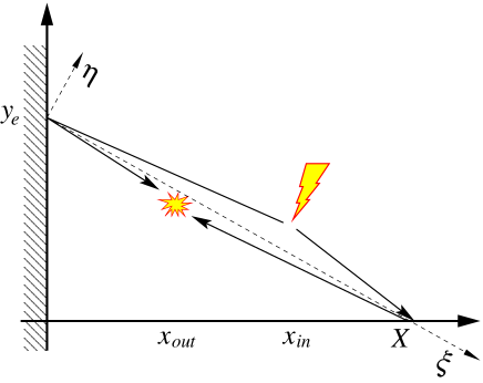
Figure 7: (Color on-line.) Electron trajectories corresponding to Raman scattering on a disordered edge. Notations are the same as in Fig. 3.

Since the edge can scatter an electron by an arbitrary angle, it is convenient to use the rotated coordinates $(\xi,\eta)$, as shown in Fig. 7. Taking the first Green’s function in Eqs. (32c), (32d) as given by Eq. (24), and taking the free Green’s functions in the paraxial approximation (i. e., assuming $|\eta|\ll\xi$), we arrive at the following expression for the Raman matrix element:

$$\mathcal{M}_{\mu} = \sqrt{\frac{\lambda_{K}}{2}}\,\frac{e^{2}v}{4\pi^{2}\omega_{in}}\times$$ (51a)

$${}\times\int\limits_{-\infty}^{\infty}{dy}_{e}\,e^{-2(\gamma/v)\sqrt{X^{2}+y_{e}^{2}}}\mathop{\mathrm{Tr}}_{2\times{2}}\{\Lambda_{\mu}{S}_{\Lambda}(y_{e})\}\times$$

$${}\times\frac{X(Xe_{in}^{y}+y_{e}e_{in}^{x})(Xe_{out}^{y}+y_{e}e_{out}^{x})^{*}}{(X^{2}+y_{e}^{2})^{3/2}}\times$$

$${}\times\int\limits_{-\infty}^{\infty}\frac{d\epsilon}{v}\int\limits_{0}^{\sqrt{X^{2}+y_{e}^{2}}}d\xi_{in}d\xi_{out}\int\limits_{-\infty}^{\infty}{d}\eta_{in}d\eta_{out}\times$$

$${}\times\sqrt{\frac{|\omega_{in}-\epsilon||\omega_{out}-\epsilon||\epsilon|^{2}}{v^{4}\xi_{in}\xi_{out}\xi_{in}^{\prime}\xi_{out}^{\prime}}}\,e^{i\Phi_{in}+i\Phi_{out}},$$

$$\Phi_{a} = \frac{|\epsilon|}{v}\left(\xi_{a}+\frac{\eta_{a}^{2}}{2\xi_{a}}\right)+\frac{|\omega_{a}-\epsilon|}{v}\left(\xi_{a}^{\prime}+\frac{\eta_{a}^{2}}{2\xi_{a}^{\prime}}\right),$$ (51b)

$$\xi_{a}^{\prime} = \sqrt{X^{2}+y_{a}^{2}}-\xi_{a},$$ (51c)

where $a$ is either “$in$” or “$out$”. Analogously to the case of the regular edge, we first integrate over $\eta_{in},\eta_{out}$, and subsequent integration over $\epsilon$ and $\xi_{in,out}$ fixes $\xi_{in}+\xi_{out}\approx\sqrt{X^{2}+y_{e}^{2}}$, $\epsilon\approx\omega_{in}/2$. As a result, we obtain

$$\mathcal{M}_{\mu} = \frac{ie^{2}}{4}\sqrt{\frac{\lambda_{K}}{2}}\int\limits_{-\infty}^{\infty}{dy}_{e}\,\mathop{\mathrm{Tr}}_{2\times{2}}\{\Lambda_{\mu}{S}_{\Lambda}(y_{e})\}\times$$ (52)

$${}\times e^{(i\omega_{in}/2+i\omega_{out}/2-2\gamma)\sqrt{X^{2}+y_{e}^{2}}/v}\times$$

$${}\times\frac{X(Xe_{in}^{y}+y_{e}e_{in}^{x})(Xe_{out}^{y}+y_{e}e_{out}^{x})^{*}}{(X^{2}+y_{e}^{2})^{2}}\times$$

$${}\times\frac{\sin[\omega_{\mathrm{ph}}\sqrt{X^{2}+y_{e}^{2}}/(2v)]}{\omega_{\mathrm{ph}}/(2v)}.$$

To calculate the intensity, we use Eqs. (23c), (23d) to average the square of the matrix element, and sum over the two phonon modes. Angular integration and summation over the two detector polarizations according to Eq. (35a) gives

$$\frac{dI_{D}}{d^{2}{\rm\bf R}} = \frac{2\lambda_{K}}{9}\left(\frac{e^{2}}{c}\right)^{2}\frac{v^{2}}{c^{2}}\,\frac{\omega_{in}/v}{L_{x}L_{y}}\int\limits_{-\infty}^{\infty}{d}y_{e}\,e^{-4\gamma\sqrt{X^{2}+y_{e}^{2}}/v}\times$$ (53a)

$${}\times\frac{\sin^{2}[\omega_{\mathrm{ph}}\sqrt{X^{2}+y_{e}^{2}}/(2v)]}{[\omega_{\mathrm{ph}}/(2v)]^{2}}\times$$

$${}\times\frac{X^{2}(X^{2}\sin^{2}\varphi_{in}+y_{e}^{2}\cos^{2}\varphi_{in})}{(X^{2}+y_{e}^{2})^{3}},$$

$$I_{D} = \frac{\pi\lambda_{K}}{36}\left(\frac{e^{2}}{c}\right)^{2}\frac{v^{2}}{c^{2}}\,\frac{\omega_{in}}{vL_{x}}\,\frac{v^{2}}{\omega_{\mathrm{ph}}^{2}}\ln\frac{\omega_{\mathrm{ph}}^{2}+(4\gamma)^{2}}{(4\gamma)^{2}}\times$$ (53b)

$${}\times\left(3\sin^{2}\varphi_{in}+\cos^{2}\varphi_{in}\right).$$

Eq. (35b) for the intensity emitted into a solid angle $$o_{out}$$ in the presence of an analyzer gives

$$I_{D} = \frac{\pi\lambda_{K}}{24}\frac{o_{out}}{4\pi}\left(\frac{e^{2}}{c}\right)^{2}\frac{v^{2}}{c^{2}}\,\frac{\omega_{in}}{vL_{x}}\,\frac{v^{2}}{\omega_{\mathrm{ph}}^{2}}\ln\frac{\omega_{\mathrm{ph}}^{2}+(4\gamma)^{2}}{(4\gamma)^{2}}\times$$

$${}\times\left[\sin^{2}\varphi_{in}+\sin^{2}\varphi_{out}+\frac{1}{2}\cos(2\varphi_{in}-2\varphi_{out})\right].$$

The trigonometric expression in the square brackets can be identically rewritten as $\sin^{2}\varphi_{in}+\sin(2\varphi_{out}-\varphi_{in})\sin\varphi_{in}+1/2$, so its absolute minimum is 1/4, reached at $\varphi_{out}=-\varphi_{in}=\pm\pi/6$.

VII.2 Excitation position dependence

Here we follow the same logic as in Sec. VI.3, but instead of Eqs. (44a)–(44c) we have

$$\frac{dI_{D}}{dt} = \frac{\lambda_{K}}{9\pi}\left(\frac{e^{2}}{c}\right)^{2}\frac{v}{c}$$ (54)

$${}\times\int\limits_{-\infty}^{\infty}dY\,dX\,dy_{e}\,e^{-4(\gamma/v)\sqrt{X^{2}+y_{e}^{2}}}\,$$

$${}\times\frac{X^{2}(X\sin\varphi_{in}+y_{e}\cos\varphi_{in})^{2}}{(X^{2}+y_{e}^{2})^{3}}$$

$${}\times\int\limits_{0}^{\sqrt{X^{2}+y_{e}^{2}}}d\xi_{in}\,d\xi_{in}^{\prime}\,e^{-i(\omega_{\mathrm{ph}}/v)(\xi_{in}-\xi_{in}^{\prime})}$$

$${}\times\mathcal{E}_{in}\!\left(\frac{\xi_{in}X}{\sqrt{X^{2}+y_{e}^{2}}},Y+y_{e}-\frac{\xi_{in}y_{e}}{\sqrt{X^{2}+y_{e}^{2}}}\right)$$

$${}\times\mathcal{E}_{in}^{*}\!\left(\frac{\xi_{in}^{\prime}X}{\sqrt{X^{2}+y_{e}^{2}}},Y+y_{e}-\frac{\xi_{in}^{\prime}y_{e}}{\sqrt{X^{2}+y_{e}^{2}}}\right),$$

where $(X,Y)$ is the point where the phonon is emitted. As in Sec. VI.3, we expand in the spatial derivatives of $\mathcal{E}_{in}({\rm\bf r})$, and obtain Eq. (46) with $l_{2}$ given by (actually, the result depends slightly on the polarization; here we choose unpolarized detection and excitation polarization along the edge, $\varphi_{in}=\pi/2$):

$$l_{2}^{2}=\ell_{\gamma}^{2}\frac{5\ln(\ell_{\gamma}/\ell_{\mathrm{ph}})-3\cdot{2}^{14}/(45\pi)^{2}}{48\ln^{2}(\ell_{\gamma}/\ell_{\mathrm{ph}})}+O(\ell_{\mathrm{ph}}^{2}).$$ (55)

This expression reproduces the experimental value $l_{2}=14\>\mbox{nm}$ if $\ell_{\gamma}=120\>\mbox{nm}$ (again, $\ell_{\mathrm{ph}}=4\>\mbox{nm}$ is taken).

VIII Raman scattering on a fragmented edge

In this section we consider the Raman scattering on an edge consisitng of armchair and zigzag segments whose typical length $d_{e}$ significantly exceeds the electronic wavelength, $d_{e}\gg\lambdabar_{\epsilon}$, where $\lambdabar_{\epsilon}=2v/\omega_{in}$. This is an intermediate case between the two limiting cases considered in the previous two sections.

Only armchair segments contribute to the Raman process.Cancado2004 Moreover, contributions from different segments add up incoherently. Thus, we first focus on the contribution of a single armchair segment, placed at $x=0$, $-d_{e}/2\leq{y}\leq{d}_{e}/2$ (as before, graphene is assumed to occupy the half-space $x>0$). The electronic Green’s function corresponding to the reflection from a single armchair segment can be easily written from the Huygens-Fresnel principle, Eq. (9) if one approximates its value on the boundary by that for an infinite perfect armchair edge:

$${G}({\rm\bf r},{\rm\bf r}^{\prime};\epsilon)=G_{0}({\rm\bf r}-{\rm\bf r}^{\prime},\epsilon)-iv\int\limits_{-d_{e}/2}^{d_{e}/2}dy_{e}$$

$$\qquad\qquad{}\times G_{0}(x,y-y_{e};\epsilon)\,\Sigma_{x}\,G_{0}(x^{\prime},y_{e}-y^{\prime};\epsilon)\,\Sigma_{y}\Lambda_{y}.$$

This approximation ignores the change of the exact wave function within the distance $\sim\lambdabar_{\epsilon}$ from the ends of the segment, which gives a small error if $d_{e}\gg\lambdabar_{\epsilon}$. In fact, it is the standard approximation for the study of diffraction in optics.BornWolf

Using this Green’s function, we obtain the following expression for the matrix element corresponding to emission of a phonon in an arbitrary point $(X,Y)$:

$$\mathcal{M}=-\sqrt{\frac{\lambda_{K}}{2}}\,\frac{e^{2}v}{\pi^{2}\omega_{in}}\int\limits_{-\infty}^{\infty}\frac{d\epsilon}{v}\int{d}^{2}{\rm\bf r}_{in}\,d^{2}{\rm\bf r}_{out}\int\limits_{-d_{e}/2}^{d_{e}/2}dy_{e}$$

$$\qquad{}\times\sqrt{\frac{|\omega_{in}-\epsilon||\omega_{out}-\epsilon|\epsilon^{2}}{v^{4}\rho_{in}\rho_{out}\rho_{in}^{\prime}\rho_{out}^{\prime}}}\,e^{i\Phi_{in}+i\Phi_{out}}$$

$$\qquad{}\times\cos\frac{\phi_{in}-\phi_{out}}{2}\sin\frac{2\varphi_{out}+\phi_{out}^{\prime}-\phi_{out}}{2}$$

$$\qquad{}\times\cos\frac{\phi_{in}^{\prime}-\phi_{out}^{\prime}}{2}\sin\frac{2\varphi_{in}+\phi_{in}^{\prime}-\phi_{in}}{2},$$ (57a)

$$\rho_{a}=\sqrt{x_{a}^{2}+(y_{a}-y_{e})^{2}},$$ (57b)

$$\rho_{a}^{\prime}=\sqrt{(X-x_{a})^{2}+(y_{a}-Y)^{2}},$$ (57c)

$$\phi_{a}=\arctan\frac{y_{a}-y_{e}}{x_{a}},\quad\phi_{a}^{\prime}=\arctan\frac{y_{a}-Y}{X-x_{a}},$$ (57d)

$$\Phi_{a}=\frac{|\epsilon|+i\gamma}{v}\,\rho_{a}+\frac{|\omega_{a}-\epsilon|+i\gamma}{v}\,\rho_{a}^{\prime},$$ (57e)

where $a$ is either “$in$” or “$out$”. It is convenient to use the paraxial approximation with respect to the axis connecting the points $(0,y_{e})$ and $(X,Y)$. In this approximation we expand

$$\rho_{a}+\rho_{a}^{\prime}\approx\frac{X}{\cos\phi_{0}}+\frac{X\cos^{3}\phi_{0}}{x_{a}(X-x_{a})}\,\frac{(y_{a}-y_{a0})^{2}}{2},$$ (58a)

$$\phi_{a}\approx\phi_{0}+\frac{y_{a}-y_{a0}}{x_{a}}\,\cos^{2}\phi_{0},$$ (58b)

$$\phi_{a}^{\prime}\approx-\phi_{0}+\frac{y_{a}-y_{a0}}{X-x_{a}}\,\cos^{2}\phi_{0},$$ (58c)

$$y_{a0}=x_{a}\tan\phi_{0},\quad\tan\phi_{0}=\frac{Y-y_{e}}{X}.$$ (58d)

Integrating over ${\rm\bf r}_{in},{\rm\bf r}_{out}$ in the usual way, we obtain

$$\mathcal{M} = -ie^{2}\sqrt{\frac{\lambda_{K}}{2}}\int\limits_{-d_{e}/2}^{d_{e}/2}dy_{e}\,\frac{\sin[\omega_{\mathrm{ph}}{X}/(2v\cos\phi_{0})]}{\omega_{\mathrm{ph}}{X}/(2v\cos\phi_{0})}$$ (59)

$${}\times\exp\left[\left(i\,\frac{\omega_{in}+\omega_{out}}{2}-2\gamma\right)\frac{X}{v\cos\phi_{0}}\right]$$

$${}\times\sin(\varphi_{in}-\phi_{0})\sin(\varphi_{out}-\phi_{0}).$$

This integral can be calculated analogously to the standard diffraction integral in optics.BornWolf According to Eq. (35a), the integrated intensity into the full solid angle $4\pi$, summed over two polarizations of the emitted photon, and integrated over ${\rm\bf R}$, is given by

$$I_{D} = \frac{8\lambda_{K}}{3}\left(\frac{e^{2}}{c}\right)^{2}\frac{v^{2}}{c^{2}}\,\frac{v}{\omega_{in}L_{x}}\,\frac{d_{e}}{L_{y}}\,\frac{\omega_{in}^{2}}{\omega_{\mathrm{ph}}^{2}}\times$$

$${}\times\left\{\sin^{2}\varphi_{in}\ln\frac{\omega_{\mathrm{ph}}^{2}+(4\gamma)^{2}}{(4\gamma)^{2}}+\cos^{2}\varphi_{in}\right.$$

$${}\qquad\times\left.\left[\frac{\omega_{\mathrm{ph}}^{2}}{\omega_{in}^{2}}\ln\frac{\omega_{in}}{\omega_{\mathrm{ph}}}+\frac{2v}{\omega_{in}d_{e}}\ln\frac{\omega_{\mathrm{ph}}^{2}+(4\gamma)^{2}}{(4\gamma)^{2}}\right]\right\}.$$

This expression is analogous to Eq. (42b), weighted by the factor $$d_{e}/L_{y} \propto\cos^{2}\varphi_{in} \varphi_{in}=0 d_{e}\gtrsim(v/\omega_{in})(\omega_{in}/\omega_{\mathrm{ph}})^{2}\approx{50}\>\mbox{nm} \omega_{in}=2\>\mbox{eV} \omega_{in}d_{e}/v\gg{1} o_{out}$$. The coefficient at the last term, , determines the minimum of the intensity at and has two contributions: the one corresponding to the infinite edge, and the one due to the finite size of the segment. The latter one is dominant unless for . Still, as long as , the ratio between the intensities for the parallel and perpendicular polarizations is large. If we use Eq. (35b) for the intensity in a solid angle in the presence of an analyzer, we obtain

$$I_{D} = 4\lambda_{K}\,\frac{o_{out}}{4\pi}\left(\frac{e^{2}}{c}\right)^{2}\frac{v^{2}}{c^{2}}\,\frac{v}{\omega_{in}L_{x}}\,\frac{d_{e}}{L_{y}}\,\frac{\omega_{in}^{2}}{\omega_{\mathrm{ph}}^{2}}\times$$

$${}\times\left\{\sin^{2}\varphi_{in}\sin^{2}\varphi_{out}\ln\frac{\omega_{\mathrm{ph}}^{2}+(4\gamma)^{2}}{(4\gamma)^{2}}\right.+$$

$${}\qquad+\left.\left[\sin^{2}(\varphi_{in}+\varphi_{out})+\frac{1}{2}\sin{2}\varphi_{in}\sin{2}\varphi_{out}\right]\right.$$

$${}\qquad\;\;\times\left.\frac{v}{\omega_{in}d_{e}}\ln\frac{\omega_{\mathrm{ph}}^{2}+(4\gamma)^{2}}{(4\gamma)^{2}}\right.+$$

$${}\qquad+\left.\cos^{2}\varphi_{in}\cos^{2}\varphi_{out}\right.$$

$${}\qquad\;\;\times\left.\left[\frac{\omega_{\mathrm{ph}}^{2}}{\omega_{in}^{2}}\ln\frac{\omega_{in}}{\omega_{\mathrm{ph}}}+\frac{v}{\omega_{in}d_{e}}\ln\frac{\omega_{\mathrm{ph}}^{2}+(4\gamma)^{2}}{(4\gamma)^{2}}\right]\right\}.$$

Eqs. (LABEL:IDfragma=), (LABEL:IDfragmb=) describe the contribution of a single armchair segment to the Raman intensity. To obtain the contribution of the whole edge, it is sufficient to multiply these expression by the total number of such segments and replace $d_{e}$ by its average, if all segments have the same orientation. It is crucial, however, that up to three different orientations of armchair segments are possible, at the angle $\pi/3$ to each other, as discussed by the author and coworkers in Ref. Casiraghi2009, .

Let us first consider a measurement in the absence of an analyzer. Since the intensity is a biliniear form of the polarization vector ${\rm\bf e}_{in}$, it can always be written in the form

$$I(\varphi_{in}) \propto \cos^{2}(\varphi_{in}-\varphi_{max})+\varepsilon\sin^{2}(\varphi_{in}-\varphi_{max})$$ (61)

$$= \frac{1+\varepsilon}{2}+\frac{1-\varepsilon}{2}\,\cos(2\varphi_{in}-2\varphi_{max}),$$

where $\varphi_{max}$ is the angle where the intensity is maximum and $\varepsilon$ is the ratio between the intensities in the minimum and in the maximum. Eq. (LABEL:IDfragma=) corresponds to $\varphi_{max}=\pi/2$ and small $\varepsilon\ll{1}$ due to the quantum diffraction.

Let the edge have $N_{0}$ armchair segments oriented along the $y$ direction, such as the one considered above, and $N_{\pm}$ segments oriented at $\pm\pi/3$ to the $y$ axis. Note that the average direction of the edge may still be arbitrary, as it depends on the distribution of zigzag segments too. Let each segment be charaterized by the same values of $\varepsilon$ and $\varphi_{max}$, when the latter is measured with respect to the corresponding normal. Adding the contributions, we again obtain an expression of the form of Eq. (61), but with different values of parameters:

$$N_{0}I(\varphi_{in})+N_{+}I(\varphi_{in}-\pi/3)+N_{-}I(\varphi_{in}+\pi/3)$$

$$\propto\cos^{2}(\varphi_{in}-\tilde{\varphi}_{max})+\tilde{\varepsilon}\sin^{2}(\varphi_{in}-\tilde{\varphi}_{max}),$$ (62a)

$$\tilde{\varphi}_{max}=\varphi_{max}+\frac{1}{2}\arctan\frac{\sqrt{3}(N_{+}-N_{-})}{2N_{0}-N_{+}-N_{-}},$$ (62b)

$$\tilde{\varepsilon}=\frac{(1+\varepsilon)N_{tot}-(1-\varepsilon)\tilde{N}}{(1+\varepsilon)N_{tot}+(1-\varepsilon)\tilde{N}},$$ (62c)

$$\tilde{N}\equiv\sqrt{N_{tot}^{2}-3(N_{+}N_{-}+N_{0}N_{+}+N_{0}N_{-})},$$ (62d)

$$N_{tot}\equiv N_{0}+N_{+}+N_{-}.$$ (62e)

Inspection of Eq. (62b) shows that $\tilde{\varepsilon}\ll{1}$ if and only if (i) $\varepsilon\ll{1}$ and (ii) $N_{tot}-\tilde{N}\ll{N}_{tot}$. The latter condition is equivalent to having one of $N_{0},N_{+},N_{-}$ to be much larger than the others. If these conditions hold, we can write (assuming that $N_{0}\gg{N}_{+},N_{-}$ for concreteness)

$$\tilde{\varepsilon}\approx\varepsilon+\frac{3}{4}\frac{N_{+}+N_{-}}{N_{0}}.$$ (63)

In the opposite case $N_{0}=N_{+}=N_{-}$ we have $\tilde{\varepsilon}=1$, so that isotropy is fully restored and no signatures of quantum diffraction are left.

An analogous summation can be performed in the presence of an analyzer in the general case, but the final expressions are very bulky and not very informative. The qualitative conclusion is the same: the terms which were small compared to the leading term $\sin^{2}\varphi_{in}\sin^{2}\varphi_{out}$ grow as one adds segments with different orientations. At $N_{0}=N_{+}=N_{-}$ the isotropy is restored,

$$\sin^{2}\varphi_{in}\sin^{2}\varphi_{out}+\sin^{2}(\varphi_{in}-\pi/3)\sin^{2}(\varphi_{out}-\pi/3)$$

$${}+\sin^{2}(\varphi_{in}+\pi/3)\sin^{2}(\varphi_{out}+\pi/3)$$

$${}=\frac{3}{8}\sin^{2}(\varphi_{in}-\varphi_{out})+\frac{9}{8}\cos^{2}(\varphi_{in}-\varphi_{out}),$$ (64)

and signatures of the quantum diffraction are lost.

Let us focus on the special case when the average direction of edge is zigzag, and it is symmetric on the average, $N_{+}=N_{0}$, $N_{-}=0$. Then we have

$$I_{D} \propto \sin^{2}\varphi_{in}\sin^{2}\varphi_{out}$$

$${}+\sin^{2}\!\left(\varphi_{in}-\frac{\pi}{3}\right)\sin^{2}\!\left(\varphi_{out}-\frac{\pi}{3}\right)+O(\varepsilon)$$

$$= \frac{3}{8}+\frac{3}{4}\cos^{2}(\varphi_{in}-\varphi_{out})$$

$${}-\cos^{2}\!\left(\varphi_{in}-\frac{\pi}{6}\right)\cos^{2}\!\left(\varphi_{out}-\frac{\pi}{6}\right)+O(\varepsilon).$$

The maximum of intensity is reached when both polarizations are along the average direction of edge. For the unpolarized detection, we add the contributions with $\varphi_{out}=0$ and $\varphi_{out}=\pi/2$ and obtain the ratio between the minimum and the maximum intensity to be $1/3+O(\varepsilon)$; if an analyzer is used and $\varphi_{in}=\varphi_{out}$, we obtain $\tilde{\varepsilon}=1/9+O(\varepsilon)$. These findings agree with the available experimental data.Gupta2009 ; Casiraghi2009

The dependence of Eq. (LABEL:IDzigzag=) has a remarkable property: at $\varphi_{in}=0$, $\varphi_{out}=\pi/3$ (or vice versa) the leading term vanishes and $I_{D}=O(\varepsilon)$, i. e. the quantum limit is still accessible. In fact, the same will be true for any edge with only two orientations of the segments (i. e, for $N_{-}=0$, but $N_{0}\neq{N}_{+}$, generally speaking). The ratio of intensity in this minimum to the maximum without analyzer is given by

$$\tilde{\varepsilon}=\frac{2}{Z}\left[\frac{v}{\omega_{in}d_{e}}+\frac{\omega_{\mathrm{ph}}^{2}}{4\omega_{in}^{2}}\,\ln\frac{\omega_{\mathrm{ph}}}{\omega_{in}}\left(\ln\frac{\omega_{\mathrm{ph}}^{2}+(4\gamma)^{2}}{(4\gamma)^{2}}\right)^{-1}\right],$$

(66a)

$$Z\equiv{1}+\frac{\sqrt{N_{0}^{2}+N_{+}^{2}-N_{0}N_{+}}}{N_{0}+N_{+}}.$$ (66b)

IX Conclusions

We have studied scattering of Dirac electrons on a graphene edge. For a translationally invariant edge (such as zigzag or armchair or another edge with a certain spatial period) the reflection can be described by an effective low-energy boundary condition for the electronic wave function.McCann2004 ; Akhmerov2008 For edges which are rough on the atomic scale we have proposed a random-matrix model which describes random scattering of electrons on the edge, respecting the particle conservation and time-reversal symmetry. Essentially, each point of the edge acts as an independent point scatterer with a random rotation of the valley state. We have also considered edges consisting of zigzag and armchair distinct segments longer than the electron wavelength, each segment can be treated as a piece of an ideal edge, while the small corrections due to quantum diffraction, can be found using the Huygens-Fresnel principle for Dirac electrons, analogously to the standard treatment of diffraction in the classical optics.

Next, we have calculated the intensity of the edge-induced $D$ peak in the Raman scattering spectrum of graphene. It is shown how the quasiclassical character of the electron motion manifests itself in the polarization dependence of the intensity. For an ideal armchair edge the maximum of intensity corresponds to the case when both the polarizer and the analyzer are along the edge, and the large ratio of intensities in the maximum and the minimum turns out to be determined by the quantum corrections to the quasiclassical motion of the photoexcited electron and the hole. For an edge consisting of randomly distributed zigzag and armchair segments of the length significantly exceeding the electron wavelength, the effect of quantum diffraction can be masked by the presence of armchair segments of different orientations. The maximum and the minimum of the intensity are determined by the number of the armchair segments with different orientations, rather than the average direction of the edge. If only two orientations of armchair segments are present in the edge, the quantum diffraction limit can still be probed by a careful choce of the polarizer and the analyzer (the polarizer should be oriented perpendicularly to one of the armchair directions, the analyzer perpendicularly to the other one). For an edge, rough at the atomic scale, no segments can be identified, and the intensity reaches its maximum for the polarization along the average direction of the edge. The ratio of the maximum and the minimum intensity is determined by the ability of the edge to scatter electrons at oblique angles.

As the whole Raman process is edge-assisted, one can pose the question about the characteristic length scale which restricts the process to the vicinity of the edge. We find that the answer is not unique, and the length scale depends on the specific observable under study. If one is interested in the total intensity or its polarization dependence, the effective length scale is $v/\omega_{\mathrm{ph}}$ ($v$ being the electronic velocity and $\omega_{\mathrm{ph}}$ the phonon frequency). However, if one makes a spatially resolved experiment, measuring the dependence of the intensity on the position of the excitation spot, the relevant length scale is the electron inelastic scattering length $v/(2\gamma)$. We have thus found a qualitative agreement with the interpretation of Ref. Novotny, , but we argued the inelastic scattering length found in that work is too large to be consistent with other available information on electron inelastic scattering in graphene.

X Acknowledgements

The author is grateful to A. C. Ferrari, S. Piscanec, and M. M. Fogler for stimulating discussions.

Appendix A Scattering matrix for an edge

The representation of the 4-column vector $\psi$, natural for scattering problems, is that of Ref. AleinerEfetov, , Eq. (5). For 4-column vectors which can be represented as a direct product

$$\left[\begin{array}[]{c}x_{1}y_{1}\\ x_{2}y_{1}\\ x_{1}y_{2}\\ x_{2}y_{2}\end{array}\right]\equiv\left[\begin{array}[]{c}x_{1}\\ x_{2}\end{array}\right]\otimes\left[\begin{array}[]{c}y_{1}\\ y_{2}\end{array}\right]\equiv\left[\begin{array}[]{c}x_{1}\\ x_{2}\end{array}\right]\otimes(y_{1}\phi_{K}+y_{2}\phi_{K^{\prime}}),$$ (67)

the $\Sigma$  matrices act on the $x$ variables, while the $\Lambda$ matrices act on the $y$ variables. The basis in the valley subspace is denoted by $\phi_{K},\phi_{K^{\prime}}$ for future convenience.

To keep the formulas compact we assume that the edge is along the $y$ direction and graphene is occupying the half-space $x>0$, i. e., ${\rm\bf n}={\rm\bf e}_{x}$. The average orientation of a disordered edge with $d_{e}\sim{a}$ does not have to be correlated with any cristallographic direction, so the description is equivalent for all orientations. Thus, expressions for a general orientation of the edge are obtained by replacing the coordinates by $x\to{\rm\bf n}\cdot{\rm\bf r}$, $y\to[{\rm\bf n}\times{\rm\bf r}]_{z}$, and the polar angles by $\varphi\to\varphi+\varphi_{\rm\bf n}$.

Let us label the eigenstates of the problem by three quantum numbers: (i) $\epsilon$, the energy of the electron; (ii) $p_{y}$, the $y$-component of the momentum of the incident plane wave (obviously, $|p_{y}|<|\epsilon|/v$), (iii) $\kappa$, the valley index (we write $\kappa=\pm{1}$ for $K$ and $K^{\prime}$, respectively). The most general wave function of such an eigenstate has the form

$$\psi_{\epsilon,{p}_{y},\kappa}(x,y)=\frac{e^{ip_{y}y-ip_{x}x}}{\sqrt{L_{x}L_{y}}}\,\sqrt{\frac{|\epsilon|}{vp_{x}}}\,\overleftarrow{\psi}_{\epsilon,{p}_{y},\kappa}+$$

$$\qquad\qquad{}+\sum_{p_{y}^{\prime}}S_{p_{y}^{\prime}p_{y}}^{\,\kappa^{\prime}\kappa}\,\frac{e^{ip_{y}^{\prime}y+ip_{x}^{\prime}x}}{\sqrt{L_{x}L_{y}}}\,\sqrt{\frac{|\epsilon|}{vp_{x}^{\prime}}}\,\overrightarrow{\psi}_{\epsilon,{p}_{y}^{\prime},\kappa^{\prime}},$$ (68a)

$$p_{x}\equiv\sqrt{(\epsilon/v)^{2}-p_{y}^{2}},\quad p_{x}^{\prime}\equiv\sqrt{(\epsilon/v)^{2}-(p_{y}^{\prime})^{2}},$$ (68b)

$$\sum_{p_{y}^{\prime}}\equiv\int\limits_{-|\epsilon|/v}^{|\epsilon|/v}\frac{L_{y}\,dp_{y}^{\prime}}{2\pi},\quad\delta_{p_{y}p_{y}^{\prime}}=\frac{2\pi}{L_{y}}\,\delta(p_{y}-p_{y}^{\prime})$$ (68c)

$$\overleftarrow{\psi}_{\epsilon,{p}_{y},\kappa}=\frac{1}{\sqrt{2}}\left[\begin{array}[]{c}e^{i(\varphi_{p_{y}}-\pi)/2}\\ e^{i(\pi-\varphi_{p_{y}})/2}\mathop{\mathrm{sgn}}\epsilon\end{array}\right]\otimes\phi_{\kappa},$$ (68f)

$$\overrightarrow{\psi}_{\epsilon,{p}_{y},\kappa}=\Sigma_{y}\overleftarrow{\psi}_{\epsilon,{p}_{y},\kappa}=\frac{1}{\sqrt{2}}\left[\begin{array}[]{c}e^{-i\varphi_{p_{y}}/2}\mathop{\mathrm{sgn}}\epsilon\\ e^{i\varphi_{p_{y}}/2}\end{array}\right]\otimes\phi_{\kappa},$$ (68i)

$$\varphi_{p_{y}}=\arctan\frac{p_{y}}{p_{x}},\quad-\frac{\pi}{2}\leq\varphi_{p_{y}}\leq\frac{\pi}{2}.$$ (68j)

The prefactor $\sqrt{|\epsilon|/(vp_{x})}$ in Eq. (68a) fixes the component of the probability current perpendicular to the boundary to be $j_{x}=-v\mathop{\mathrm{sgn}}\epsilon/(L_{x}L_{y})$ for the incident wave.holes Finally, ${S}_{p_{y}^{\prime}p_{y}}^{\,\kappa^{\prime}\kappa}$ are the scattering matrix elements, which may depend on $\epsilon$. Note that $\varphi_{p_{y}}=\varphi_{p_{y}^{\prime}}$ corresponds to the specular reflection. The wave functions $\psi_{\epsilon,{p}_{y},\kappa}(x,y)$ are orthogonal,

$$\int\limits_{-\infty}^{\infty}{d}y\int\limits_{0}^{\infty}{dx}\,\psi^{\dagger}_{\epsilon,p_{y},\kappa}(x,y)\,\psi_{\epsilon^{\prime}\!,p_{y}^{\prime},\kappa^{\prime}}(x,y)=$$

$$=\frac{2\pi{v}}{L_{x}}\,\delta(\epsilon-\epsilon^{\prime})\,\delta_{p_{y}p_{y}^{\prime}}\,\delta_{\kappa\kappa^{\prime}},$$ (69)

provided that the scattering matrix is unitary:

$$\sum_{p_{y}^{\prime},\kappa^{\prime}}\left({S}^{\,\kappa^{\prime}\kappa}_{p_{y}^{\prime}p_{y}}\right)^{*}{S}^{\,\kappa^{\prime}\kappa^{\prime\prime}}_{p_{y}^{\prime}p_{y}^{\prime\prime}}=\delta_{\kappa\kappa^{\prime\prime}}\,\delta_{p_{y}p_{y}^{\prime\prime}}.$$ (70)

The same condition ensures the conservation of the flux, i. e. that the current $j_{x}=v\mathop{\mathrm{sgn}}\epsilon/(L_{x}L_{y})$ for the scattered part of the wave function (68a). Reflection from a regular edge with wave function given by Eq. (15), corresponds to ${S}^{{\kappa^{\prime}\kappa}}_{p_{y}^{\prime}p_{y}}=\delta_{p_{y}^{\prime}p_{y}}\phi_{\kappa^{\prime}}^{\dagger}{S}_{\Lambda}\phi_{\kappa}$.

The time reversal symmetry imposes another condition on the scattering matrix (reciprocity condition). Namely, the time-reversed wave function $U_{t}\psi_{\epsilon,{p}_{y},\kappa}^{*}(x,y)$ describes an eigenstate of the problem, and thus it must be a linear combination of $\psi_{\epsilon,{p}_{y}^{\prime},\kappa^{\prime}}(x,y)$ with different $p_{y}^{\prime},\kappa^{\prime}$. Noting that

$$U_{t}\overleftarrow{\psi}^{*}_{\epsilon,-p_{y},-\kappa}=i\kappa\overrightarrow{\psi}_{\epsilon,p_{y},\kappa},$$ (71a)

$$U_{t}\overrightarrow{\psi}^{*}_{\epsilon,-p_{y},-\kappa}=-i\kappa\overleftarrow{\psi}_{\epsilon,p_{y},\kappa}.$$ (71b)

we obtain the reciprocity condition,

$$S^{\,\kappa^{\prime}\kappa}_{p_{y}^{\prime}p_{y}}=-\kappa\kappa^{\prime}\,S^{-\kappa,-\kappa^{\prime}}_{-p_{y},-p_{y}^{\prime}},$$ (72)

which can also be written in the matrix form as $S_{p_{y}^{\prime}p_{y}}=-\Lambda_{y}\,S^{T}_{-p_{y},-p_{y}^{\prime}}\Lambda_{y}$, where $S^{T}$ denotes the $2\times{2}$ matrix transpose.

To relate the scattering matrix to the $T$-matrix in Eq. (21), we compare the $x\gg{v}/|\epsilon|$ asymptotics of the corresponding wave functions. The Green’s function $G_{0}({\rm\bf r}-{\rm\bf r}_{e},\epsilon)$ entering Eq. (21) can be represented as follows:

$$\begin{split}&G_{0}(x,y-y_{e},\epsilon)=\\ &=\int\limits_{-\infty}^{\infty}\frac{d\epsilon^{\prime}}{2\pi{v}}\int\limits_{-|\epsilon^{\prime}|/v}^{|\epsilon^{\prime}|/v}\frac{dp_{y}}{2\pi}\,\frac{|\epsilon^{\prime}|}{vp_{x}}\,\frac{e^{ip_{y}(y-y_{e})}}{\epsilon-\epsilon^{\prime}+i0^{+}\mathop{\mathrm{sgn}}\epsilon}\\ &{}\times\sum_{\kappa}\left(\overrightarrow{\psi}_{\epsilon^{\prime},{p}_{y},\kappa}\overrightarrow{\psi}_{\epsilon^{\prime},{p}_{y},\kappa}^{\dagger}e^{ip_{x}x}+\overleftarrow{\psi}_{\epsilon^{\prime},{p}_{y},\kappa}\overleftarrow{\psi}_{\epsilon^{\prime},{p}_{y},\kappa}^{\dagger}e^{-ip_{x}x}\right),\end{split}$$ (73)

where we suppressed the damping $\gamma_{\epsilon}\to{0}^{+}$ and denoted $p_{x}\equiv\sqrt{(\epsilon^{\prime}/v)^{2}-p_{y}^{2}}$). To determine the $x\gg{v}/|\epsilon|$ asymptotics of the Green’s function, we shift the $\epsilon^{\prime}$ integration contour in the upper (lower) complex half-plane at $\epsilon^{\prime}>0$ ($\epsilon^{\prime}<0$) for the term $\propto{e}^{ip_{x}x}$, and in the lower (upper) half-plane at $\epsilon^{\prime}>0$ ($\epsilon^{\prime}<0$) for the term $\propto{e}^{-ip_{x}x}$. The magnitude $\epsilon^{\prime\prime}$ of the shift is such that $v/x\ll\epsilon^{\prime\prime}\ll|\epsilon^{\prime}|$ As a result, (i) the contribution from the term $\propto{e}^{-ip_{x}x}$ will be exponentially small except for the small region near zero, $|\epsilon^{\prime}|\sim{v}/x$; (ii) the contribution from the term $\propto{e}^{ip_{x}x}$ will be determined by the pole $\epsilon^{\prime}=\epsilon+i0^{+}\mathop{\mathrm{sgn}}\epsilon$, the rest of the contour contributing an exponentially small quantity; (iii) the contribution from $|\epsilon^{\prime}|\sim{v}/x$ will be small as $v/(|\epsilon|x)$. Thus, at $x\gg{v}/|\epsilon|$ we arrive at

$$G_{0}(x,y-y_{e},\epsilon) = \frac{i}{v}\int\limits_{-|\epsilon|/v}^{|\epsilon|/v}\frac{dp_{y}}{2\pi}\,\frac{\epsilon}{vp_{x}}\,{e}^{ip_{y}(y-y_{e})+ip_{x}x}$$ (74)

$${}\times\sum_{\kappa}\overrightarrow{\psi}_{\epsilon,{p}_{y},\kappa}\overrightarrow{\psi}_{\epsilon,{p}_{y},\kappa}^{\dagger}.$$

Substituting this expression and the first term of Eq. (15) into Eq. (24), and comparing the result with last term of Eq. (15), we obtain the relation

$$S_{p_{y}^{\prime}p_{y}}^{\,\kappa^{\prime}\kappa} = \frac{i\mathop{\mathrm{sgn}}\epsilon}{v}\int\frac{dy_{e}}{L_{y}}\,e^{-i(p_{y}^{\prime}-p_{y})y_{e}}$$ (75)

$${}\times\frac{\overrightarrow{\psi}_{\epsilon,{p}_{y}^{\prime},\kappa^{\prime}}^{\dagger}T(\varphi_{p_{y}^{\prime}},\pi-\varphi_{p_{y}};y_{e})\overleftarrow{\psi}_{\epsilon,{p}_{y},\kappa}}{\sqrt{\cos\varphi_{p_{y}^{\prime}}\,\cos\varphi_{p_{y}}}}.$$

Here $\varphi_{p_{y}^{\prime}}$ is the polar angle of the direction ${\rm\bf s}$, and $\pi-\varphi_{p_{y}}$ is the polar angle of the incident momentum ${\rm\bf p}$, directed towards the edge. Using Eqs. (71a), (71b), one can establish the equivalence between the reciprocity condition, Eq. (72), and Eq. (22). Using the unitarity condition, Eq. (70), one fixes the prefactor $\pi{v}/|\epsilon|$ in front of the $\delta$-function in Eq. (23d).

Appendix B Integrals of Sec. VI.2

First, let us focus on Eq. (40a) for $\mathcal{M}_{\|}$. Upon integration over $y_{in},y_{out}$, it takes the following form:

$$\mathcal{M}_{\|} = \frac{e^{2}}{\omega_{in}}\,\sqrt{\frac{4\lambda_{K}v}{i\pi}}\int\limits_{-\infty}^{\infty}\frac{d\epsilon}{v}\int\limits_{0}^{X}dx_{in}\,dx_{out}\,e^{i\Phi_{x}-2\gamma{X}/v}$$ (76a)

$${}\times\left(\frac{x_{in}+x_{out}}{|\epsilon|}+\frac{X-x_{in}}{|\omega_{in}-\epsilon|}+\frac{X-x_{out}}{|\omega_{out}-\epsilon|}\right)^{-1/2},$$

$$\Phi_{x} = \frac{|\epsilon|}{v}\,(x_{in}+x_{out})+\frac{|\omega_{in}-\epsilon|}{v}\,(X-x_{in})$$ (76b)

$${}+\frac{|\omega_{out}-\epsilon|}{v}\,(X-x_{out}).$$

If one neglects the square root and integrates first over $x_{in}$, the energy is constrained to be $\epsilon\approx\omega_{in}/2$ with the precision $\sim{v}/X$. If one integrates over $x_{out}$, then $\epsilon\approx\omega_{out}/2$ (which is not inconsistent with the previous condition as long as $X\sim{v}/\omega_{\mathrm{ph}}$). If one also removes the moduli and integrates over $\epsilon$, then $x_{in}+x_{out}\approx{X}$.

To implement these observations more rigorously, let us introduce new variables,

$$\tilde{x}=\frac{x_{in}+x_{out}-X}{2},\quad x_{0}=x_{in}-x_{out},$$ (77a)

$$\tilde{\epsilon}=\epsilon-\frac{\omega_{in}+\omega_{out}}{4},$$ (77b)

$$\Phi_{x}=4\,\frac{\tilde{\epsilon}\tilde{x}}{v}-\frac{\omega_{\mathrm{ph}}{x}_{0}}{2v}+\frac{\omega_{in}+\omega_{out}}{2v}\,X.$$ (77c)

Recalling that the typical scale of the $\tilde{\epsilon}$ dependence of the rest of the integrand is $\omega_{in}$, and that of the $\tilde{x}$ dependence is $X$, we rewrite

$$4\,\frac{\tilde{\epsilon}\tilde{x}}{v}=\frac{\omega_{in}X}{v}\left(\frac{\tilde{\epsilon}}{\omega_{in}}+\frac{\tilde{x}}{X}\right)^{2}-\frac{\omega_{in}X}{v}\left(\frac{\tilde{\epsilon}}{\omega_{in}}-\frac{\tilde{x}}{X}\right)^{2}.$$ (78)

Taking the two expressions in the brackets as new integration variables, we can use the stationary phase approximation justified by $\omega_{in}X/v\gg{1}$. As a result, the integral is contributed by $|\tilde{\epsilon}|\sim\sqrt{\omega_{in}v/X}\ll\omega_{in}$ and by $|\tilde{x}|\sim\sqrt{Xv/\omega_{in}}\ll{X}$. Thus, in the rest of the integrand they can be simply set to zero, i. e. we approximate $e^{4i\tilde{\epsilon}\tilde{x}/v}\approx(\pi{v}/2)\delta(\tilde{\epsilon})\delta(\tilde{x})$. The remaining integration over $x_{0}$ is elementary:

$$\int\limits_{-X}^{X}dx_{0}\int\limits_{-(X-|x_{0}|)/2}^{(X-|x_{0}|)/2}d\tilde{x}\int\limits_{|\tilde{\epsilon}|\lesssim\omega_{in}/2}\frac{d\tilde{\epsilon}}{v}\,e^{i\Phi_{x}}$$

$$\approx\pi{e}^{i(\omega_{in}+\omega_{out})X/(2v)}\,\frac{\sin[\omega_{\mathrm{ph}}{X}/(2v)]}{\omega_{\mathrm{ph}}/(2v)}.$$ (79)

For the integral in Eqs. (43a), (43b) we have:

$$\tilde{x}=\frac{x_{in}-x_{out}-X}{2},\quad x_{0}=\frac{x_{in}+x_{out}-X}{2},$$ (80a)

$$\tilde{\epsilon}=\epsilon-\frac{\omega_{in}+\omega_{out}}{4},$$ (80b)

$$\Phi_{x}^{\prime}=-2\,\frac{\tilde{\epsilon}\tilde{x}}{v}+\frac{\omega_{\mathrm{ph}}{x}_{0}}{v}+\frac{\omega_{in}X}{v}.$$ (80c)

$$\int\limits_{|\tilde{\epsilon}|\lesssim\omega_{in}/2}\frac{d\tilde{\epsilon}}{v}\,\int\limits_{0}^{X}d\tilde{x}\int\limits_{-\tilde{x}/2}^{\tilde{x}/2}dx_{0}\,e^{i\Phi_{x}^{\prime}}$$

$$=e^{i\omega_{in}X/v}\int\limits_{|\tilde{\epsilon}|\lesssim\omega_{in}/2}\frac{v\,d\tilde{\epsilon}}{2\omega_{\mathrm{ph}}}$$

$$\times\left[\frac{e^{-i(2\tilde{\epsilon}-\omega_{\mathrm{ph}}/2)X/v}-1}{2\tilde{\epsilon}-\omega_{\mathrm{ph}}/2}-(\omega_{\mathrm{ph}}\to-\omega_{\mathrm{ph}})\right].$$ (81)

If we extend the limits of the $\tilde{\epsilon}$ integration to infinity, the integral vanishes by analyticity. Thus, it is determined by the region $|\epsilon|\sim\omega_{in}$ and can be estimated as $\sim{v}/\omega_{in}$.

Now let us pass to the derivation of Eq. (41b) for $\mathcal{M}_{\perp}$. The difference from the previous case is that integration over $y_{in},y_{out}$ in the derivation is more subtle. Namely, we encounter oscillating integrals of the kind $\int{y}^{2}e^{i\alpha{y}^{2}}dy$. This integral is assigned the value $\sqrt{\pi/4}\,(-i\alpha)^{-3/2}$, which may be understood as the analytical continuation from the upper complex half-plane of $\alpha$. One may argue that since the integral is divergent for real $\alpha$, it is determined by $|y|\sim{1}/\sqrt{\mathop{\mathrm{Im}}\alpha}$ which are not small, so the expansion to $y^{2}$ both in the exponential and in the pre-exponential factor is not valid.

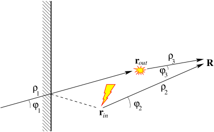
Figure 8: (Color on-line.) Geometry corresponding to Eq. (82). The solid black arrows show the vectors ${\rm\bf\rho}_{1},{\rm\bf\rho}_{2},{\rm\bf\rho}_{3}$.

Let us write down the expression for the matrix element without using the paraxial approximation [we omit the $1/\zeta$ terms of the expansion in Eq. (8) as they do not produce $y^{2}$ terms and do not represent any convergence problem],

$$\mathcal{M} = \sqrt{\frac{i\lambda_{K}}{\pi^{3}v}}\,\frac{e^{2}}{\omega_{in}}\int\limits_{-\infty}^{\infty}\frac{d\epsilon}{v}\int d^{2}{\rm\bf r}_{in}\,d^{2}{\rm\bf r}_{out}\,\cos\frac{\varphi_{2}-\varphi_{3}}{2}$$ (82)

$${}\times\sin\frac{2\varphi_{in}+\varphi_{1}-\varphi_{2}}{2}\sin\frac{2\varphi_{out}-\varphi_{1}-\varphi_{3}}{2}$$

$${}\times{e}^{(i|\epsilon|-\gamma)\rho_{1}/v+(i|\omega_{in}-\epsilon|-\gamma)\rho_{2}/v+(i|\omega_{out}-\epsilon|-\gamma)\rho_{3}/v}$$

$${}\times\sqrt{\frac{|(\omega_{in}-\epsilon)(\omega_{out}-\epsilon)\epsilon|}{\rho_{1}\rho_{2}\rho_{3}}}.$$

The distances $\rho_{1,2,3}$ and the angles $\varphi_{1,2,3}$ are shown in Fig. 8. Again, integration over $\epsilon/v$ gives effectively $\delta(\rho_{1}-\rho_{2}-\rho_{3})$, so the exponential in the integrand becomes $e^{(i\omega_{in}-2\gamma)\rho_{2}/v+(i\omega_{out}-2\gamma)\rho_{3}/v}$. The phase of this exponential is rapidly oscillating, and the stationary phase condition gives precisely $y_{in},y_{out}\to{0}$. The straightforward application of the stationary phase method for $\varphi_{in}=\varphi_{out}=0$ is impeded by the presence of two sine functions in front of the exponential.

First of all, let us check the convergence of the integral at large distances, i. e. assuming $r_{in},r_{out}\gg{X}$. Then it is convenient to use the polar coordinates for ${\rm\bf r}_{in},{\rm\bf r}_{out}$ whose polar angles are almost $\pi+\varphi_{2},\pi+\varphi_{3}$. The $\delta$-function fixes $\varphi_{2}=\pi-\varphi_{1}$, $\varphi_{3}=\pi+\varphi_{1}$. We can set $X=0$ everywhere except the Jacobian:

$$\rho_{1}\approx{r}_{in}r_{out}-\frac{r_{in}r_{out}}{2(r_{in}+r_{out})}\,(\varphi_{2}+\varphi_{3})^{2},$$ (83a)

$$\rho_{2,3}\approx{r}_{in,out}+X\cos\varphi_{2,3},$$ (83b)

$$\delta(\rho_{1}-\rho_{2}-\rho_{3})\approx\sqrt{\frac{r_{in}+r_{out}}{Xr_{in}r_{out}}}\,\delta(\varphi_{2}+\varphi_{3}).$$ (83c)

This gives a finite value,

$$\mathcal{M} = \sqrt{\frac{i\lambda_{K}}{\pi^{3}v}}\,\frac{e^{2}}{\omega_{in}}\int\limits_{-\pi/2}^{\pi/2}d\varphi_{1}\int r_{in}\,dr_{in}\,r_{out}\,dr_{out}$$ (84)

$${}\times\sqrt{\frac{r_{in}+r_{out}}{Xr_{in}r_{out}}}\,\sqrt{\frac{(\omega_{in}/2)^{3}}{(r_{in}+r_{out})r_{in}r_{out}}}$$

$${}\times{e}^{(i\omega_{in}-2\gamma)r_{in}/v+(i\omega_{out}-2\gamma)r_{out}/v}$$

$${}\times\cos\varphi_{1}\cos(\varphi_{in}+\varphi_{1})\cos(\varphi_{out}-\varphi_{1})$$

$$\approx \sqrt{\frac{i\lambda_{K}e^{4}}{8\pi^{3}}\frac{v}{\omega_{in}X}}\,\frac{v}{\omega_{in}}$$

$${}\times\left(\frac{2}{3}\,\sin\varphi_{in}\sin\varphi_{out}-\frac{4}{3}\,\cos\varphi_{in}\cos\varphi_{out}\right).$$

Note that for any polarization it is smaller than $\mathcal{M}_{\|}$ from Eq. (41a) by a factor $\omega_{\mathrm{ph}}/\omega_{in}$.

Thus, we are facing a situation of the kind

$$F(\alpha)=\int\limits_{-\infty}^{\infty}f(y)\,e^{i\alpha\Phi(y)}\,dy,$$ (85)

where (i) the function $\Phi(y)$ is growing as $|y|$ at $|y|\to\infty$ and has an extremum at $y=0$, where it can be expanded as $\Phi(y)=\Phi(0)+\Phi^{\prime\prime}(0)\,y^{2}/2+O(y^{4})$, (ii) $\alpha$ is large and is assumed to have a positive imaginary part, and (iii) $f(y)=f^{\prime\prime}(0)\,y^{2}/2+O(y^{3})$ at $y\to{0}$, while the behavior of the function $f(y)$ at $|y|\to\infty$ is such that the in the limit $\mathop{\mathrm{Im}}\alpha\to{0}$ the integral $F(\alpha)$ remains finite. Then $F(\alpha)$ is analytic in the upper complex half-plane of $\alpha$. Thus, the expansion

$$F(\alpha)=\frac{\sqrt{\pi/2}\,f^{\prime\prime}(0)}{[-i\alpha\Phi^{\prime\prime}(0)]^{3/2}}+O((-i\alpha)^{-5/2}),$$ (86)

established for large positive imaginary $\alpha$, holds in the whole upper half-plane, including the vicinity of the real axis. The two-dimensional integration over $y_{in},y_{out}$, leading to Eq. (41b) is fully analogous.

Appendix C Detailed expressions for Sec. VI.3

Note that length $l_{2}$ is not well defined in the general case. Namely, for an arbitrary kernel $\mathcal{K}(x,x^{\prime})$ and an arbitrary shape of $\mathcal{E}_{in}(x)$ the expansion in the derivatives of $\mathcal{E}_{in}(x)$ does not automatically “wrap” into the expansion in the derivatives of $w(x)$, Eq. (46). However, $l_{2}$ can be defined in two particular cases which are most important for us. It is convenient to introduce an auxiliary notation: for an arbitrary function $\mathcal{F}(x,x^{\prime})$ we define

$$\langle\langle\mathcal{F}(x,x^{\prime})\rangle\rangle\equiv\int\limits_{0}^{\infty}\mathcal{F}(x,x^{\prime})\,\mathcal{K}(x,x^{\prime})\,\frac{dx\,dx^{\prime}}{l_{0}^{2}}-\mathcal{F}(l_{1},l_{1}).$$ (87)

One case when the length $l_{2}$ can be defined is when the kernel $\mathcal{K}(x,x^{\prime})$ is such that

$$\langle\langle{x}^{2}\rangle\rangle+\langle\langle(x^{\prime})^{2}\rangle\rangle=2\langle\langle{xx^{\prime}}\rangle\rangle,$$ (88)

then one can set $l_{2}=\sqrt{\langle\langle{xx^{\prime}}\rangle\rangle}$. For the kernel given by Eq. (44c) this property holds in the limit $\ell_{\gamma}\gg\ell_{\mathrm{ph}}$:

$$\int\limits_{0}^{\infty}{x}^{2}\mathcal{K}(x,x^{\prime})\,dx\,dx^{\prime}=-2\ell_{\mathrm{ph}}^{4}\ln\frac{\ell_{\gamma}^{2}+4\ell_{\mathrm{ph}}^{2}}{4\ell_{\mathrm{ph}}^{2}}$$

$$\qquad{}+\ell_{\gamma}^{2}\ell_{\mathrm{ph}}^{2}\,\frac{\ell_{\gamma}^{4}-4i\ell_{\gamma}^{3}\ell_{\mathrm{ph}}+20\ell_{\gamma}^{2}\ell_{\mathrm{ph}}^{2}+32\ell_{\mathrm{ph}}^{4}}{4(\ell_{\gamma}^{2}+4\ell_{\mathrm{ph}}^{2})^{2}},$$ (89)

$$\int\limits_{0}^{\infty}{x}x^{\prime}\mathcal{K}(x,x^{\prime})\,dx\,dx^{\prime}=\ell_{\mathrm{ph}}^{4}\ln\frac{\ell_{\gamma}^{2}+4\ell_{\mathrm{ph}}^{2}}{4\ell_{\mathrm{ph}}^{2}}$$

$$\qquad{}+\frac{\ell_{\gamma}^{2}\ell_{\mathrm{ph}}^{2}}{4}\,\frac{\ell_{\gamma}^{2}-4\ell_{\mathrm{ph}}^{2}}{\ell_{\gamma}^{2}+4\ell_{\mathrm{ph}}^{2}},$$ (90)

The second case when $l_{2}$ can be defined is the gaussian profile $\mathcal{E}_{in}(x)\propto{e}^{-(x-x_{0})^{2}/(2L^{2})}$, which has a special property $\mathcal{E}_{in}^{\prime\prime}(x)\mathcal{E}_{in}(x)=[\mathcal{E}_{in}^{\prime}(x)]^{2}-[\mathcal{E}_{in}(x)]^{2}/L^{2}$. Then the difference between the left-hand and the right-hand sides of Eq. (88) can be absorbed in the overall coefficient, so that instead of Eq. (44c) we have its slightly modified version:

$$\mathcal{I}_{x_{0}}=Al_{0}^{2}\left[w(l_{1}-x_{0})+\frac{l_{2}^{2}}{2}\,w^{\prime\prime}(l_{1}-x_{0})\right]+O(\ell^{3}/L^{3}),$$

(91a)

$$A=1-\frac{\langle\langle{x}^{2}\rangle\rangle+\langle\langle(x^{\prime})^{2}\rangle\rangle-2\langle\langle{xx^{\prime}}\rangle\rangle}{4L^{2}},$$ (91b)

$$l_{2}^{2}=\frac{\langle\langle{x}^{2}\rangle\rangle+\langle\langle(x^{\prime})^{2}\rangle\rangle+2\langle\langle{xx^{\prime}}\rangle\rangle}{4}=$$

$$\quad=\frac{\ell_{\gamma}^{2}(\ell_{\gamma}^{4}+10\ell_{\gamma}^{2}\ell_{\mathrm{ph}}^{2}+8\ell_{\mathrm{ph}}^{4})}{4(\ell_{\gamma}^{2}+4\ell_{\mathrm{ph}}^{2})^{2}}\left(\ln\frac{\ell_{\gamma}^{2}+4\ell_{\mathrm{ph}}^{2}}{4\ell_{\mathrm{ph}}^{2}}\right)^{-1}$$

$$\qquad{}-\frac{\ell_{\gamma}^{6}}{4(\ell_{\gamma}^{2}+4\ell_{\mathrm{ph}}^{2})^{2}}\left(\ln\frac{\ell_{\gamma}^{2}+4\ell_{\mathrm{ph}}^{2}}{4\ell_{\mathrm{ph}}^{2}}\right)^{-2}-\frac{\ell_{\mathrm{ph}}^{2}}{2}.$$ (91c)

References

- (1) K. S. Novoselov, A. K. Geim, S. V. Morozov, D. Jiang, Y. Zhang, S. V. Dubonos, I. V. Grigorieva, and A. A. Firsov, Science 306, 666 (2004).
- (2) A. K. Geim and K. S. Novoselov, Nature Materials 6, 183 (2007).
- (3) X. Lu, H. Huang, N. Nemchuk, and R. S. Ruoff, Appl. Phys. Lett. 75, 193 (1999).
- (4) M. Y. Han, B. Özyilmaz, Y. Zhang, and P. Kim, Phys. Rev. Lett. 98, 206805 (2007).
- (5) Z. Chen, Y.-M. Lin, M. J. Rooks, and P. Avouris, Physica E 40, 228 (2007).
- (6) L. A. Ponomarenko, F. Schedin, M. I. Katsnelson, R. Yang, E. W. Hill, K. S. Novoselov, and A. K. Geim, Science 320, 356 (2008).
- (7) S. Schnez, F. Molitor, C. Stampfer, J. Güttinger, I. Shorubalko, T. Ihn, and K. Ensslin, Appl. Phys. Lett. 94, 012107 (2009).
- (8) K. Todd, H.-T. Chou, S. Amasha, and D. Goldhaber-Gordon, Nano Lett. 9, 416 (2009).
- (9) Z. Klusek, Z. Waqar, E. A. Denisov, T. N. Kompaniets, I. V. Makarenko, A. N. Titkov, and A. S. Bhatti, Appl. Surf. Sci. 161, 508 (2000).
- (10) Y. Kobayashi, K.-i. Fukui, T. Enoki, and K. Kusakabe, and Y. Kaburagi, Phys. Rev. B 71, 193406 (2005).
- (11) Y. Kobayashi, K.-i. Fukui, T. Enoki, and K. Kusakabe, Phys. Rev. B 73, 125415 (2006).
- (12) J. Campos-Delgado, J. M. Romo-Herrera, X. Jia, D. A. Cullen, H. Muramatsu, Y. A. Kim, T. Hayashi, Z. Ren, D. J. Smith, Y. Okuno, T. Ohba, H. Kanoh, K. Kaneko, M. Endo, H. Terrones, M. S. Dresselhaus, and M. Terrones, Nano Lett. 8, 2773 (2008).
- (13) Z. Liu, K. Suenaga, P. J. F. Harris, and S. Iijima, Phys. Rev. Lett. 102, 015501 (2009).
- (14) K. A. Ritter and J. W. Lyding, Nature Mat. 8, 235 (2009).
- (15) L. G. Cançado, M. A. Pimenta, B. R. A. Neves, M. S. S. Dantas, and A. Jorio, Phys. Rev. Lett. 93, 247401 (2004).
- (16) L. G. Cançado, R. Beams, and L. Novotny, arXiv:0802.3709.
- (17) Y. You, Z. Ni, T. Yu, and Z. Shen, Appl. Phys. Lett. 93, 163112 (2008).
- (18) A. K. Gupta, T. J. Russin, H. R. Gutièrrez, and P. C. Eklund, Nano Lett. 3, 45 (2009).
- (19) C. Casiraghi, A. Hartschuh, H. Qian, S. Piscanec, C. Georgi, K. S. Novoselov, D. M. Basko, and A. C. Ferrari, Nano Lett. (in press).
- (20) C. Thomsen and S. Reich, Phys. Rev. Lett. 85, 5214 (2000).
- (21) S. E. Stein and R. L. Brown, J. Am. Chem. Soc. 109, 3721 (1987).
- (22) K. Tanaka, S. Yamashita, H. Yamabe, and T. Yamabe, Synth. Met. 17, 143 (1987).
- (23) M. Fujita, M. Yoshida, and K. Nakada, Fullerene Sci. Technol. 4, 565 (1996).
- (24) M. Fujita, K. Wakabayashi, K. Nakada, and K. Kusakabe, J. Phys. Soc. Jpn. 65, 1920 (1996).
- (25) K. Nakada, M. Fujita, G. Dresselhaus, and M. S. Dresselhaus, Phys. Rev. B 54, 17954 (1996).
- (26) E. McCann and V. I. Fal’ko, J. Phys.: Condens. Matter 16, 2371 (2004).
- (27) A. R. Akhmerov and C. W. J. Beenakker, Phys. Rev. B 77, 085423 (2008).
- (28) D. A. Areshkin, D. Gunlycke, and C. T. White, Nano Lett. 7, 204 (2007).
- (29) E. Louis, J. A. Vergés, F. Guinea, and G. Chiappe, Phys. Rev. B 75, 085440 (2007).
- (30) D. Querlioz, Y. Apertet, A. Valentin, K. Huet, A. Bournel, S. Galdin-Retailleau, and P. Dollfus, Appl. Phys. Lett. 92, 042108 (2008).
- (31) M. Evaldsson, I. V. Zozoulenko, H. Xu and T. Heinzel, Phys. Rev. B 78, 161407(R) (2008).
- (32) T. Fang, A. Konar, H. Xing, and D. Jena, Phys. Rev. B 78, 205403 (2008).
- (33) G. Tkachov, Phys. Rev. B 79, 045429 (2009).
- (34) G. C. Brown, V. Celli, M. Haller, and A. Marvin, Surf. Sci. 136, 381 (1984).
- (35) A. R. McGurn, A. A. Maradudin, and V. Celli, Phys. Rev. B 31, 4866 (1985).
- (36) G. Brown, V. Celli, M. Haller, A. A. Maradudin, and A. Marvin, Phys. Rev. B 31, 4993 (1985).
- (37) N. Garcia and E. Stoll, J. Opt. Soc. Am. A 2, 2240 (1985).
- (38) P. Tran and V. Celli, J. Opt. Soc. Am. A 5, 1635 (1988).
- (39) A. A. Maradudin, E. R. Méndez, and T. Michel, Opt. Lett. 14, 151 (1989).
- (40) A. A. Maradudin, T. Michel, A. R. McGurn, and E. R. Méndez, Ann. Phys. (N.Y.) 203, 255 (1990).
- (41) M. Born and E. Wolf, Principles of Optics (Cambridge University Press, 1999).
- (42) D. M. Basko, Phys. Rev. B 76, 081405(R) (2007).
- (43) D. M. Basko, Phys. Rev. B 78, 125418 (2008).
- (44) Note that one does not need to invoke any singularity in the phonon density of states to explain the maximum intensity for the polarization along the edge, as it was done in the literature.Cancado2004 Moreover, such a singularity would not rule out trajectories like that shown in Fig. 2(b).
- (45) A less successful attempt of a similar measurement was also recently published in Ref. Gupta2009, . However, in this work even the excitation profile width was known only up to an uncertainty of 50 nm. In this case one cannot extract reliably quantitative information about smaller length scales.
- (46) S. Piscanec, M. Lazzeri, F. Mauri, A. C. Ferrari, and J. Robertson, Phys. Rev. Lett. 93, 185503 (2004).
- (47) J. Yan, Y. Zhang, P. Kim, and A. Pinczuk, Phys. Rev. Lett. 98 166802 (2007).
- (48) S. Pisana, M. Lazzeri, C. Casiraghi, K. S. Novoselov, A. K. Geim, A. C. Ferrari, and F. Mauri, Nature Mat. 6, 198 (2007).
- (49) D. M. Basko and I. L. Aleiner, Phys. Rev. B 77, 041409(R) (2008).
- (50) M. Calandra and F. Mauri, Phys. Rev. B 76, 205411 (2007).
- (51) M. Lazzeri, C. Attaccalite, L. Wirtz, and F. Mauri, Phys. Rev. B 78, 081406(R) (2008).
- (52) A. C. Ferrari, J. C. Meyer, V. Scardaci, C. Casiraghi, M. Lazzeri, F. Mauri, S. Piscanec, D. Jiang, K. S. Novoselov, S. Roth, and A. K. Geim, Phys. Rev. Lett. 97, 187401 (2006).
- (53) F. Tuinstra and J. L. Koenig, J. Chem. Phys. 53, 1126 (1970).
- (54) S. Knight and W. B. White, J. Mater. Res. 4, 385 (1989).
- (55) M. J. Matthews, M. A. Pimenta, G. Dresselhaus, M. S. Dresselhaus, and M. Endo, Phys. Rev. B 59, R6585 (1999).
- (56) L. G. Cançado, K. Takai, T. Enoki, M. Endo, Y. A. Kim, H. Mizusaki, A. Jorio, L. N. Coelho, R. Magalhães-Paniago, and M. A. Pimenta, Appl. Phys. Lett. 88, 163106 (2006).
- (57) L. G. Cançado, A. Jorio, and M. A. Pimenta, Phys. Rev. B 76, 064304 (2007).
- (58) The author is aware of only one past calculation of the Raman scattering intensity in graphene nanocrystallites [K. Sato, R. Saito, Y. Oyama, J. iang, L. G. Cançado, M. A. Pimenta, A. Jorio, Ge. G. Samsonidze, G. Dresselhaus, and M. S. Dresselhaus, Chem. Phys. Lett. 427, 117 (2006)]. However, it gave , failing to reproduce the experimental dependence.
- (59) A. C. Ferrari and J. Robertson, Phys. Rev. B 61, 14095 (2000).
- (60) G. A. Zickler, B. Smarsly, N. Gierlinger, H. Peterlik, and O. Paris, Carbon 44, 3239 (2006).
- (61) E. McCann, K. Kechedzhi, V. I. Fal’ko, H. Suzuura, T. Ando, and B. L. Altshuler, Phys. Rev. Lett. 97, 146805 (2006).
- (62) I. L. Aleiner and K. B. Efetov, Phys. Rev. Lett. 97, 236801 (2006).
- (63) L. Brey and H. A. Fertig, Phys. Rev. B 73, 235411 (2006).
- (64) For the states with the direction of the electron group velocity is opposite to that of momentum. Thus, for the first term of the wave function (68a) represents an outgoing flux of electrons, and the second term – to an incoming flux. However, we prefer to work with the chronologically ordered Green’s function , defined in Eq. (6), rather than for the retarded Green’s function , the analytical continuation of from the positive semiaxis of through the upper complex half-plane of . For this purpose we work with the solutions (68a) where the first term of the wave function (68a) represents an incoming flux for electrons if and for holes if .