A proposed testbed for detector tomography

Abstract

Measurement is the only part of a general quantum system that has yet to be characterized experimentally in a complete manner. Detector tomography provides a procedure for doing just this; an arbitrary measurement device can be fully characterized, and thus calibrated, in a systematic way without access to its components or its design. The result is a reconstructed POVM containing the measurement operators associated with each measurement outcome. We consider two detectors, a single-photon detector and a photon-number counter, and propose an easily realized experimental apparatus to perform detector tomography on them. We also present a method of visualizing the resulting measurement operators.

I Introduction

A quantum protocol or experiment can be divided into three stages: preparation, processing, and measurement. Quantum state tomography Smithey et al. (1993); Dunn et al. (1995); White et al. (1999) and process tomography Childs et al. (2001); Mitchell et al. (2003) respectively prescribe a procedure to completely characterize the first two stages, and have been successfully demonstrated experimentally. State tomography has played a crucial role in identifying and visualizing novel quantum states White et al. (2001); Lvovsky et al. (2001). Process tomography is critical for verifying the operation of quantum logic gates O’Brien et al. (2004) and characterizing decoherence processes Myrskog et al. (2005). Completing this triad, detector tomography is a procedure for determining the POVM (positive operator-valued measure) set of an arbitrary quantum detector Luis and Sánchez-Soto (1999). Thus, without any knowledge of the inner workings of the detector we could predict its response to any input. To the best of our knowledge, detector tomography has not been demonstrated. Here, we propose an experimental testbed capable of performing detector tomography on measurement devices acting in the Fock space of the optical mode (i.e., the photon number Hilbert space). Precise knowledge of the detection POVM set is beneficial for measurement driven quantum information processing, such as cluster-state computing Raussendorf and Briegel (2001). It is also critical for state and process tomography, which use the measurement as a reference. Recently, it has also been shown that one can perform enhanced measurements by projecting onto non-classical states with a detector Resch et al. (2007a, b). Without any need for a theoretical model of the detector, detector tomography can establish which states the detector projects onto, possibly establishing whether they are indeed non-classical.

We will begin by introducing the general experimental and theoretical requirements for performing detector tomography. We will then describe the detectors which we aim to characterize using our proposed testbed. Following this, we will provide a description of the testbed we have proposed to characterize the aforementioned detectors. Finally, we outline a method of visualizing the POVM elements in terms of Wigner quasi-probability distributions.

II Detector Tomography

Detector tomography is a method of experimentally determining the POVM associated with the detector. A theoretical description of detector tomography was introduced by Luis and Sánchez-Soto in Ref. Luis and Sánchez-Soto (1999) in 1999, a maximum-likelihood technique was applied in Ref. Fiurasek (2001) in 2001, ancilla-assisted detector tomography was considered in 2004 in Ref. D’Ariano et al. (2004), and an optimal processing scheme devised in 2007 in Ref. D’Ariano and Perinotti (2007).

In elementary quantum mechanics, a measurement is described by a Hermitian operator $\hat{A}$ which can be decomposed into a sum of projectors $\hat{\pi}_{i}$ with weights $\lambda_{i}$, where each projector corresponds to an outcome of the measurement:

$$\hat{A}=\sum_{i}\lambda_{i}\hat{\pi}_{i}.$$ (1)

These projectors $\hat{\pi}_{i}$ are often deduced by the action of the measuring device in the classical regime. For example, since a calcite crystal spatially separates the polarization components of a laser beam it is reasoned to act similarly at the quantum level on single photons (i.e., $\hat{\pi}_{1}=\left|H\right\rangle\left\langle H\right|$ and $\hat{\pi}_{2}=\left|V\right\rangle\left\langle V\right|$, horizontal and vertical polarization projectors aligned with the axes of the calcite). This example is justified by a theoretical model, namely quantum-electrodynamics, which shows the classical field reduces to field operators at the quantum level. However, some measurements, such as Bell-state measurement Mitchell et al. (2003) or single-photon detection, cannot be traced back to any classical device. These quantum detectors typically rely on an unsystematic combination of a theoretical model (e.g., semiconductor theory) and detector characterizations of limited scope (e.g., of the detector noise and efficiency). In contrast, detector tomography would provide a systematic method, with minimal assumptions, to characterize these quantum detectors and, thus, predict their action on an general input state.

The most general type of quantum measurement is described by a POVM, a set of positive-semidefinite operators $O_{\alpha}$ corresponding to the measurement outcomes. These generalized measurements are uniquely quantum in the sense that they have no analogue in the classical regime. For instance, any POVM can be implemented by coupling the measured system to an ancilla system and then performing projective measurements on the combined system Peres (1990); the coupling has the potential to create entanglement between the two systems, which is impossible in the classical regime.

In some ways, detector tomography is very similar to the established procedure of state tomography. In state tomography, one begins with an ensemble of systems prepared identically in state $\hat{\rho}$. A measurement $\hat{O}_{\alpha}$, is performed on a subset of the ensemble for the purpose of estimating the probability $p_{\alpha}$:

$$p_{\alpha}=\mathrm{Tr}(\hat{O}_{\alpha}\hat{\rho}).$$ (2)

This is repeated for a set of measurements $\{\hat{O}_{\alpha}\}$, producing a set of estimated probabilities $\{p_{{}_{\alpha}}\}$. Through Eq. (2) and the precise knowledge of the form of each measurement $\hat{O}_{\alpha}$, one can estimate $\hat{\rho}$. Significantly, the role of $\hat{O}_{\alpha}$ and $\hat{\rho}$ are symmetric in Eq. (2). This means that with a set of known input states $\{\hat{\rho}_{\alpha}\}$ one could instead estimate an unknown measurement $\hat{O}$ through Eq. (2), which is the goal of detector tomography.

Despite these similarities, state and detector tomography have some important differences. One obvious difference is that the former seeks to reconstruct a single operator, $\hat{\rho}$, whereas the latter seeks to reconstruct a set of operators $\{\hat{O}_{\gamma}\},\gamma=1,\ldots,D$, where $D$ is the number of measurement outcomes. Both the density matrices and the POVM elements must be positive-semidefinite and, hence, Hermitian. However, density matrices have a unit trace, whereas a POVM element does not. Instead, a POVM set $\{\hat{O}_{\gamma}\}$ must satisfy,

$$\sum_{\gamma=1}^{D}\hat{O}_{\gamma}=\hat{\mathbbm{1}},$$ (3)

where $\hat{\mathbbm{1}}$ is the identity, ensuring that the probabilities for all the measurement outcomes sum to one. This has implications for mathematical strategies for reconstruction, such as maximum likelihood, where Eqs. (2) and (3) must be included as constraints on the reconstructions.

Generally, in tomography one requires what is known as a “tomographically complete” set to reference against. In state tomography, this translates to a set of reference measurements $\{\hat{O}_{\alpha}\}$ that span the $d^{2}-1$ dimensional Hilbert-Schmidt space of the density matrix (the $-1$ term comes from the unit trace constraint). In detector tomography, the reference states $\{\hat{\rho}_{\alpha}\}$ must span the Hilbert-Schmidt space of the POVM set. A spanning set will necessarily have at least $d^{2}$ elements in it. To determine if a particular $d^{2}$ sized subset of the total set spans the space, one first vectorizes each element in the subset, then stacks these row vectors into a matrix, and then calculates the determinant. If the determinant is nonzero this subset is a spanning set and hence, the set of reference states (or reference measurements, in the case of state tomography) is tomographically complete. We shall consider an example later in the paper.

III The detectors

Before performing detector tomography, one needs to analyze the detectors in order to identify the Hilbert space they function in, and then find a suitable set of input states. We propose a testbed for two types of related detectors: the avalanche photodiode (APD), and the time-multiplexing detector (TMD).

APDs are photodiodes that use the avalanche effect (i.e., impact ionization leading to the exponential multiplication of carriers) to achieve sensitivity to single photons. These detectors have the remarkable ability to detect a single photon. Unfortunately, if more than one photon is detected this information is lost in the avalanche. Hence, this detector acts as a binary detector; the two possible detection outcomes are detection of at least one photon (click) and the detection of no photons (no click). For each photon impinging on the detector there is an intrinsic efficiency of the detector $\eta_{\text{APD}}$ that the photon will cause an avalanche. The probability of detecting at least one out of $n$ photons is given by

$$P(\text{{click}})_{n}=1-\left(1-\eta_{\text{APD}}\right)^{n},$$ (4)

and the probability of detecting none of the $n$ photons is,

$$P(\text{{no click}})_{n}=\left(1-\eta_{\text{APD}}\right)^{n}.$$ (5)

Thus, there is a non-zero probability of getting a no click event, even with photons hitting the detector. The detection can be approximated with the two POVM elements,

no click : $$\hat{O}_{0}=\sum_{n=0}^{\infty}\left(1-\eta_{\text{APD}}\right)^{n}\left|n\right\rangle\left\langle n\right|,$$ (6)

click $$: \hat{O}_{1}=\hat{\mathbbm{1}}-\sum_{n=0}^{\infty}\left(1-\eta_{\text{APD}}\right)^{n}\left|n\right\rangle\left\langle n\right|.$$ (7)

These approximate POVM elements do not include effects such as dark counts, afterpulsing, and detector saturation. The contributions from dark counts and afterpulsing can cause detection events without an actual photon being present. They will increase the values of the $\hat{O}_{1}$ matrix elements. However since dark counts are independent of the actual count rate they should predominantly affect the matrix elements at low photon numbers. Conversely, afterpulsing is dependent on a counting event happening before, and thus, would be more prominent for higher photon numbers. Detector saturation would manifest itself by a dependence of $\eta_{\text{APD}}$ on $n$. These effects would have to be included in a more complicated detector model if one desired to derive more realistic POVM elements. Previous experiments with APDs Coldenstrodt-Ronge and Silberhorn (2007) indicate that these approximate POVM elements will be a reasonable model on which to design a testbed.

Several schemes have been proposed to overcome the lack of photon number resolution with APDs Paul et al. (1996); Kok and Braunstein (2001); Banaszek and Walmsley (2003). In a time multiplexing detector, the pulse under investigation is split into several spatial and temporal bins and then detected with APDs Achilles et al. (2003); Coldenstrodt-Ronge and Silberhorn (2007); Fitch et al. (2003). The principle of operation of our implementation is depicted in Figure 1.

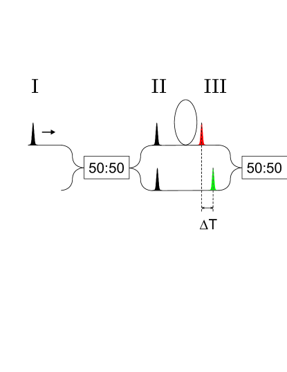
Figure 1: Schematic of a time multiplexed detector. The incoming pulse ($\mathbf{I}$) is split at a 50:50 beam splitter. The resulting pulses ($\mathbf{II}$) are partially delayed ($\mathbf{III}$) and then split again ($\mathbf{IV}$). The initial input pulse ($\mathbf{I}$) ends up in several temporal and spatial bins ($\mathbf{IV}$), which are then detected with APDs.

The pulse under investigation ($\mathbf{I}$) is split at a beamsplitter and one of the two spatial modes ($\mathbf{II}$) is delayed with respect to the other one ($\mathbf{III}$). The two spatial modes are then recombined at a beamsplitter, resulting in two temporal modes in each of the spatial outputs of the beamsplitter ($\mathbf{IV}$). Additional delay stages can be added to further increase the number of temporal modes. We propose to perform detector tomography on a TMD with two delay stages, resulting in a total of eight output bins. The advantage of splitting the incoming pulse into many bins is that if the pulse contains several photons these may be distributed into different bins and, thus, counted as individual photons by APDs. The measurement result of the TMD is the number of click events summed over all the bins. Thus, for our detector, with two stages, there are nine outcomes, 0 to 8 clicks. Unfortunately, $k$ clicks does not imply there were only $k$ photons at the TMD input. Photons may end up in the same bin and, thus, result in fewer clicks than the number of photons in the input pulse. Photons also suffer from losses in the TMD and the detection efficiency of the APDs. While this introduces an uncertainty in the measurement outcome on a shot-to-shot basis, for an ensemble measurement of the same quantum state the resulting click-statistics grasped in the vector ${p}$ can be related to the photon number statistics as a vector ${\sigma}$ of the input state by

$${p}=\mathbf{C}\cdot\mathbf{L}{\sigma},$$ (8)

where $\mathbf{L}$ represents the losses in the system and $\mathbf{C}$ is called the convolution matrix, which accounts for several photons ending up in the same bin after splitting. The loss matrix can be calculated by combining all losses in the system and modeling them as a single beam splitter with reflectivity $\eta_{\text{loss}}$ at the front of the fiber network Silberhorn et al. (2004); Achilles et al. (2006) as,

$$\mathbf{L}_{n\prime n}=\begin{cases}\binom{n}{n\prime}\left(1-\eta_{\text{loss}}\right)^{n\prime}\eta_{\text{loss}}^{n-n\prime}&\text{if:\ }n\geqslant n\prime\\ 0&\text{otherwise,}\end{cases}$$ (9)

with $n,n\prime\in 0,\dots,N$. This simply describes the probability of $n\prime$ out of $n$ photons being transmitted. For the convolution matrix one has to take into account all possible routes a photon could take through the fiber network Achilles et al. (2004) and the matrix elements can be calculated as follows:

$$\mathbf{C}_{k,n}=\begin{cases}0,&k>n,\\ \sum_{b}p_{b_{1}}p_{b_{2}}\cdots p_{b_{n}},&k=n,\\ \sum_{b}\left[\sum_{c}\frac{1}{{\operatorname{id}(c)!}}\prod_{j=1}^{k}\binom{n-\sum_{l=0}^{j-1}c_{l}}{c_{j}}p_{b_{1}}^{c_{1}}p_{b_{2}}^{c_{2}}\cdots p_{b_{k}}^{c_{k}}\right],&k<n.\end{cases}$$ (10)

In reality, the beamsplitters used in the TMD are never exactly 50% reflective due to variation in their manufacture. For a $N$-bin TMD, $p_{1},\ldots,p_{N}$ are the probabilities of a single photon exiting from the fiber network in a particular bin. While these probabilities would all be equal in the case of 50/50 beamsplitters, we set them by calibration measurements using an intense laser input pulse. The first two lines of Eq. (10) correspond to the straightforward cases of more photons being detected than entering the detector (for which the probability is zero, if dark counts and afterpulsing are negligible) and detecting all incoming photons respectively. In the third case, $k<n$, all possible combinations of distributing these $n$ photons into the bins have to be taken into account. These different combinations are represented by the $k$-tuples $b=\left(b_{1},b_{2},\cdots,b_{k}\right)$ with $b_{i}\in 1,\dots,N$ and $b_{1}\neq b_{2}\neq\cdots\neq b_{k}$. Some of the bins can be occupied by more than one photon. All possible distributions of the photons across the bins are described by the possible partitions of $n$ into $k$ parts. These can be represented by $k$-tuples $c=\left(c_{1},c_{2},\cdots,c_{k}\right)$ with $c_{i}\in\{1,\dots,n\},\text{and }c_{1}\geqslant c_{2}\geqslant\cdots\geqslant c_{k}$, $\sum_{k}c_{k}=n$, and the definition $c_{0}=0$. For each bin, one has to consider all possible ways in which the $c_{j}$ photons ending up in this particular bin can be choosen. With the photons remaining to be distributed given by $n-\sum_{l=0}^{j-1}c_{l}$, the binomial coefficient in Eq. (10) accounts for this. However, if some of the elements of the tuple $c$ are equal, the binomial coefficient will overestimate the number of distributions. Bins occupied with the same number of photons are not distinguishable, but are counted separately. This must be corrected for by dividing by the number of permutations these bins can form, i.e., the factorial of the number of bins with equal number of photons. We denote this by $\operatorname{id}(c)!$. For example for the tuple $c=\left(4;4;2;2;2;1\right)$, $\operatorname{id}(c)!=2!\cdot 3!$.

For the eight bin TMD that we plan to use in the proposed detector tomography scheme, the convolution matrix was calculated using classical measurements of the probabilities $p_{1},\ldots,p_{N}$ and reads:

$$\mathbf{C}=\begin{pmatrix}1&0&0&0&0&0&0&0&0\\ 0&1&0.128&0.017&0.000&0.000&0.000&0.000&0.000\\ 0&0&0.872&0.334&0.101&0.028&0.008&0.002&0.001\\ 0&0&0&0.649&0.496&0.265&0.123&0.053&0.022\\ 0&0&0&0&0.402&0.509&0.422&0.290&0.181\\ 0&0&0&0&0&0.198&0.375&0.444&0.423\\ 0&0&0&0&0&0&0.073&0.193&0.308\\ 0&0&0&0&0&0&0&0.018&0.063\\ 0&0&0&0&0&0&0&0&0.002\\ &&&&&&&&\end{pmatrix}.$$ (11)

The matrices developed above actually contain the POVM elements describing the TMD. We expect these POVM elements to be diagonal in the photon number basis since the TMD has no phase reference and, thus, no sensitivity to off-diagonal coherences. In Eq. (8), the matrix $\mathbf{C}\cdot\mathbf{L}$ represents the reaction of the detector to different numbers of incoming photons. When the matrix $\mathbf{CL}$ acts on a photon number distribution ${\sigma}$, the probability of a particular measurement outcome is found by taking an inner product of ${\sigma}$ with the corresponding row of the matrix. This action is similar to the action of the trace in Eq. (2), as we will demonstrate explicitly. This allows us to identify the rows of $\mathbf{C}\cdot\mathbf{L}$ as the diagonals of the TMD’s POVM:

$$\hat{O}_{j}=\begin{bmatrix}\left[\mathbf{C}\cdot\mathbf{L}\right]_{j,0}&0&0&0&0\\ 0&\ddots&0&0&0\\ 0&0&\left[\mathbf{C}\cdot\mathbf{L}\right]_{j,i}&0&0\\ 0&0&0&\ddots&0\\ 0&0&0&0&\left[\mathbf{C}\cdot\mathbf{L}\right]_{j,N}\end{bmatrix},$$ (12)

where $j$ is the $j$-clicks outcome, and $\left[\mathbf{C}\cdot\mathbf{L}\right]_{j,i}$ is the value in the $j$th row and $i$th column of $\mathbf{C}\cdot\mathbf{L}$. The density matrix of the incoming quantum state is related to ${\sigma}$ via,

$$\hat{\rho}=\begin{bmatrix}\sigma_{0}&\rho_{0,1}&\cdots&\rho_{0,N}\\ \rho_{1,0}&\sigma_{1}&\cdots&\rho_{1,N}\\ \vdots&\vdots&\ddots&\vdots\\ \rho_{N,0}&\rho_{N,1}&\cdots&\sigma_{N}\end{bmatrix},$$ (13)

expressed in the number basis, where the $i$th element of ${\sigma}$ is $\sigma_{i}$. We leave the off-diagonal elements of $\hat{\rho}$ as undetermined, since they do not contribute after the trace. Using this form we evaluate the trace in Eq. (2):

$$\mathrm{Tr}(\hat{O}_{j}\hat{\rho}) =\mathrm{Tr}\left(\begin{bmatrix}\left[\mathbf{C}\cdot\mathbf{L}\right]_{j,0}&0&0&0&0\\ 0&\ddots&0&0&0\\ 0&0&\left[\mathbf{C}\cdot\mathbf{L}\right]_{j,i}&0&0\\ 0&0&0&\ddots&0\\ 0&0&0&0&\left[\mathbf{C}\cdot\mathbf{L}\right]_{j,N}\end{bmatrix}\cdot\begin{bmatrix}\sigma_{0}&\rho_{0,1}&\cdots&\rho_{0,N}\\ \rho_{1,0}&\sigma_{1}&\cdots&\rho_{1,N}\\ \vdots&\vdots&\ddots&\vdots\\ \rho_{N,0}&\rho_{N,1}&\cdots&\sigma_{N}\end{bmatrix}\right)$$ (14)

$$=\mathrm{Tr}\left(\begin{bmatrix}\left[\mathbf{C}\cdot\mathbf{L}\right]_{j,0}\cdot\sigma_{0}&0&0&0&0\\ 0&\ddots&0&0&0\\ 0&0&\left[\mathbf{C}\cdot\mathbf{L}\right]_{j,i}\cdot\sigma_{i}&0&0\\ 0&0&0&\ddots&0\\ 0&0&0&0&\left[\mathbf{C}\cdot\mathbf{L}\right]_{j,N}\cdot\sigma_{N}\end{bmatrix}\right)$$ (15)

$$=\sum_{i=0}^{N}\left[\mathbf{C}\cdot\mathbf{L}\right]_{j,i}\cdot\sigma_{i}=p_{j}.$$ (16)

This last line is equivalent to Eq. (8), as we expected.

As we have shown, one can derive a theoretical POVM set to describe a time-multiplexed detector. However, as with the APD, this is a simplified description of the POVM and does not include afterpulsing (which can result in a click from one time bin triggering a click in the next), dark counts in the APDs at the outputs, as well as imperfections in the counting electronics (which can be considerably complicated).

In summary, the APD and the TMD perform their measurements in the Fock space of the optical mode. Furthermore, both detectors have POVMs that are expected to be diagonal in the photon-number basis. Since this confines their action to a subspace of the Fock space, it should allow us to simplify the tomography. For the APDs all photon numbers apart from zero photons are combined into a single detection event and, to a first approximation, the only detector parameter is the efficiency. This makes the APD a rather simple detector and a theoretical model of their POVM elements was easily calculated. Thus, APDs would be the first detector with which we propose to demonstrate a proof of principle detector tomography. The TMD, on the other hand, is non-trivial to describe, with both the loss and the convolution matrix having complicated forms. Incorporating realistic APDs into this model would be challenging, if not impossible. Consequently, the TMD is the second detector that we propose to perform detector tomography on. It is a suitable candidate for a serious test of the detector tomography procedure. We propose to compare the reconstructed POVM set to the theoretical ones derived above to check how accurate our detector models really are.

IV The proposed testbed

To perform tomography of these two detectors, we need probe states in the Fock space. We must also identify a set of states that span the space of the detector operators, i.e., a tomographically complete set. Since neither detector possesses a phase-reference (such as a local oscillator), we make the safe assumption for our proposed testbed that the off-diagonal components of $\{\hat{O}_{\gamma}\}$ for each detector are zero in the photon-number basis. It follows that each $\hat{O}_{\gamma}$ contains $d$ free parameters, one for each diagonal element, where $d$ is the the dimension of the Hilbert space. The tomographically complete set will then contain at least $d$ input states. Unfortunately, the photon number representation of the Hilbert space is infinite, and so we must truncate it at some point for our mathematical reconstruction. This truncation sets the $d$ we shall use in the tomography testbed we propose. A good point to set this truncation at is in the region in which the detector behavior has saturated to a constant. e.g. We expect the TMD’s response to 100 photons and 101 photons will be nearly identical (outcome 8-clicks with $\approx 100\%$ probability), making $d=100$ a good place to truncate. Since we do not require sensitivity to inter-photon coherences a naturally tomographically complete set of input states $\{\hat{\rho}_{\alpha}\}$ for our proposed testbed is the Fock states. Each input Fock state would allow us to determine the corresponding diagonal element in each of the TMD’s measurement operators $\{\hat{O}_{\gamma}\}.$ However, Fock states are difficult to produce with high fidelity. Fortunately, another candidate, the coherent state, is straightforward to produce with high-fidelity.

Apart from being the quantum state that most resembles a classical state, coherent states have a unique property under attenuation: in the photon-number basis, a coherent state $|\alpha\rangle$ can be written,

$$|\alpha\rangle=\sum_{n=0}^{\infty}{{\exp}\left({-\frac{|\alpha|^{2}}{2}}\right)\frac{\alpha^{n}}{\sqrt{n!}}|n\rangle,}$$ (17)

which results in a Poissonian photon-number distribution. With attenuation $1-\eta$, the coherent state transforms according to,

$$\hat{U}_{\eta}|\alpha\rangle=|\eta\alpha\rangle=\sum_{n=0}^{\infty}{{\exp}\left({-\frac{\eta|\alpha|^{2}}{2}}\right)\frac{\left(\sqrt{\eta}\alpha\right)^{n}}{\sqrt{n!}}|n\rangle.}$$ (18)

This is another coherent state with a lower mean number of photons. This property is important for the creation of known states in the low photon number regime, a necessity for tomography on single photon detectors. Specifically, the high-fidelity coherent states produced by a laser could be easily attenuated to power levels suitable for the tomography while still retaining their form. Attenuation also reduces the impact of technical noise in the laser. The fractional uncertainty in the photon number of a coherent state, ${\Delta{n}}/{\langle n\rangle}$, is - once it is attenuated to a low photon level - much higher than the pulse-to-pulse jitter of the pulse energy of our laser source (typical values around $2\%$). This suggests that the use of coherent states would also be reasonably robust against technical noise.

It is well known, that a continuous set of coherent probe state vectors $|\alpha\rangle$ form a basis for the Fock space,

$$|\psi\rangle=\int d\alpha|\alpha\rangle\langle\alpha|\psi\rangle.$$ (19)

However it is not as clear that they form a basis for the Hilbert-Schmidt space. The proof that they do lies in the existence of the P-function $P(\alpha)$:

$$\hat{\rho}=\int P(\alpha)|\alpha\rangle\langle\alpha|d^{2}\alpha.$$ (20)

However, we expect to use a discrete subset of coherent states $|\alpha\rangle_{i}$ rather than the full continuous basis for our proposed detector tomography testbed. We now attempt to find if this reduced set is tomographically complete. We vectorize $d$ coherent states density matrices $\left|\alpha_{i}\right\rangle\left\langle\alpha_{i}\right|,$ $i=1,\ldots,d$, keeping only the diagonals (since our detector POVM set is contained within this subspace). Stacking these row vectors into a matrix, we find,

$$\begin{bmatrix}\left|\left\langle 0|\alpha_{1}\right\rangle\right|^{2}&\left|\left\langle 1|\alpha_{1}\right\rangle\right|^{2}&\ldots&\left|\left\langle d|\alpha_{1}\right\rangle\right|^{2}\\ \left|\left\langle 0|\alpha_{i}\right\rangle\right|^{2}&\ddots&&\\ \vdots&&\ddots&\\ \left|\left\langle 0|\alpha_{d}\right\rangle\right|^{2}&&&\left|\left\langle d|\alpha_{d}\right\rangle\right|^{2}\end{bmatrix}.$$ (21)

The next step, finding the determinant, is difficult to do in general. Instead we consider a specific set of $d=10$ reference coherent states, in evenly spaced steps from $|\alpha_{1}|^{2}=1$ to $|\alpha_{10}|^{2}=10$. The determinant

$${\det}\left(\begin{bmatrix}0.37&0.37&0.18&0.06&0.02&0.00&0.00&0.00&0.00&0.00\\ 0.14&0.27&0.27&0.18&0.09&0.04&0.01&0.00&0.00&0.00\\ 0.05&0.15&0.22&0.22&0.17&0.10&0.05&0.02&0.01&0.00\\ 0.02&0.07&0.15&0.20&0.20&0.16&0.10&0.06&0.03&0.01\\ 0.01&0.03&0.08&0.14&0.18&0.18&0.15&0.10&0.07&0.04\\ 0.00&0.01&0.04&0.09&0.13&0.16&0.16&0.14&0.10&0.07\\ 0.00&0.01&0.02&0.05&0.09&0.13&0.15&0.15&0.13&0.10\\ 0.00&0.00&0.01&0.03&0.06&0.09&0.12&0.14&0.14&0.12\\ 0.00&0.00&0.01&0.02&0.03&0.06&0.09&0.12&0.13&0.13\\ 0.00&0.00&0.00&0.01&0.02&0.04&0.06&0.09&0.11&0.13\end{bmatrix}\right)\neq 0,$$ (22)

implying that this set is tomographically complete, for a space truncated at photon number basis state $n=d$. Consequently, it appears that a finite set of coherent states are a good set of reference states for our proposed detector tomography testbed.

An essential requirement for a tomography system is precise and accurate knowledge of the probe states. In the context of our proposed testbed, this translates to knowing $\alpha$ accurately. Keeping in mind that $|\alpha|^{2}$ will be less than $100$, a direct measurement is out of reach of commercial power meters. For a coherent state the mean number of photons $\langle n\rangle$ is connected to $\alpha$ via,

$$\langle n\rangle=|\alpha|^{2}.$$ (23)

For pulsed light of the wavelength $\lambda$ and the repetition frequency $f$ the time averaged power $P$ can be calculated by,

$$P=\frac{\langle n\rangle hcf}{\lambda},$$ (24)

which then enables a calculation of $|\alpha|^{2}$ from the measured power:

$$|\alpha|^{2}=\frac{P\lambda}{hcf}.$$ (25)

While $\lambda$ and $f$ can generally be determined accurately, P cannot. Systematic error in the power measurement would result in a global scaling of the detector response: the reconstructed “efficiency” of the detector would scale by the error, while the form of the POVM element would remain unchanged. We expect this $|\alpha|^{2}$ systematic error to be less than 5%. For $|\alpha|^{2}=1$, $\lambda=800$ nm and $f=100$ kHz (experimental parameters, we plan to run the proposed tomography on), $P=25$ attoWatts, a strikingly low average power. However, since coherent states are invariant under attenuation, a highly transmissive beamsplitter could be used to pick off a large portion of the incoming beam. If the ratio of power in the transmitted and reflected arms is well calibrated, the high power arm can be used to monitor the power in the low power arm. This can leverage the power into the microWatt range, accessible to power meters with calibrations that can be traced to a National Standards Institute. In our proposed testbed, this beamsplitter would be placed after a variable attenuator, used to set $\alpha$, as depicted in Figure 2. For phase-sensitive detectors, a tomographically complete set of input states could be generated simply by adding a variable path length for the coherent state in the testbed, to phase shift $\alpha$, i.e., $\alpha\mapsto\alpha e^{i\phi}$.

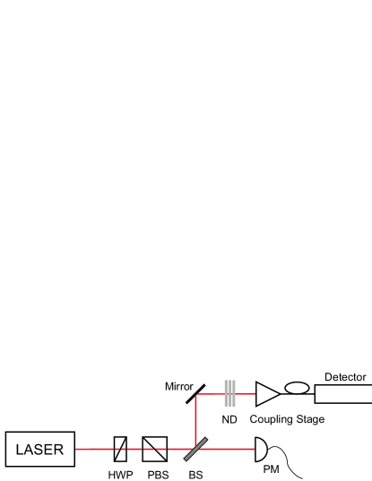
Figure 2: Schematic of our detector testbed. A probe beam undergoes variable attenuation realized with a half waveplate (HWP) and a polarizing beamsplitter (PBS). A large portion of the beam is split of at a beamsplitter (BS) and detected by a power meter (PM) to monitor the variable attenuation, while the smaller portion of the beam is further attenuated with neutral density filters (ND) and then coupled into the detector under investigation.

We simulated the tomography of a TMD with our proposed testbed by using the model given in Eq. (8). We used the convolution matrix for our TMD displayed in Eq. (11) and simulated a detector tomography using 400 different values of $|\alpha|^{2}$ for the reference states, ranging from $|\alpha|^{2}=0$ to $|\alpha|^{2}=40$. In Figure 3, we plot the probabilities of both the 1-click and 5-click outcomes against the $|\alpha|^{2}$ of the probe state. The curves for the 1-click and the 5-click outcomes have very different shapes with small overlap: while the 1-click exhibits a well defined peak for low $|\alpha|^{2}$, the 5-click peak is much broader and has a maximum at higher $|\alpha|^{2}$. This shows that different measurement outcomes are associated with easily distinguishable responses to a spanning set of input $\alpha,$ suggesting that the mathematical inversion from the estimated probabilities (e.g., with Eq. (2)) is practical.

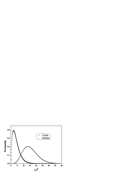
Figure 3: Simulation of a detector tomography for the TMD. 400 different values of $|\alpha|^{2}$ between $|\alpha|^{2}=0$ and $|\alpha|^{2}=40$ were simulated. A comparison between the 1-click and the 5click element shows a small overlap and smaller peak for the 1-click element, while the 5-click element is broader and peaked at higher photon number.

An analogous tomography device exists in the area of Homodyne State Tomography: the eight-port homodyne system. This device projects the unknown state onto a coherent state, much the same as our proposed testbed. It has been pointed out that reconstruction of the density matrix from the measured data in an eight-port homodyne system is an ill-conditioned problem Leonhardt (1997). Noise in the measured data causes the inversion of Eq. (3) to have large errors, indicating that while coherent states form a tomographically complete basis, they are still deficient for tomography. Considering noise from counting statistics, in detector tomography the data set size is limited only by the repetition rate of the laser, which can be as high as 80 MHz. Thus, we can quickly accumulate enough data such that counting errors for each outcome are insignificant. However, sources of noise, other than from counting, can hamper inversion. To counter the effect of these a common strategy is to introduce some amount of regularization to the inversion Boyd and Vandenberghe (2004). Often, this regularization is implicit in the reconstruction, as in the Radon Transformation or Pattern Functions used in two-port homodyne tomography, which introduce smoothing of the data Raymer and Beck (2004). Indeed, filtering of data is a common technique established in the origins of tomography in medical computer imaging. These techniques have yet to be used in detector tomography, but we expect their application will be fruitful.

V A phase-space representation of the POVM

A common complaint about quantum tomography is that the end result is difficult to interpret physically O’Brien et al. (2004); Lanyon et al. (2007); Rhode (2005); Mitchell et al. (2003). For example, in process tomography the reconstructed map for the process has $d^{2}\times d^{2}$ elements for a $d$ dimensional Hilbert space and thus quickly becomes too large to understand upon inspection. A reconstructed POVM set can similarly contain a large number of independent parameters, $(D-1)\times d^{2}$ if there are $D$ measurement outcomes. However, the measurement operators $\{\hat{O}_{\gamma}\}$ benefit from their mathematical similarities to density states, allowing us to apply many of the same representation methods. Our detectors operate in the Fock space, which can be represented in the $x$ and $p$ basis, where $x$ and $p$ are the normalized electric field quadratures. This points to a particularly appealing representation commonly used to represent the state of a field mode, the Wigner function.

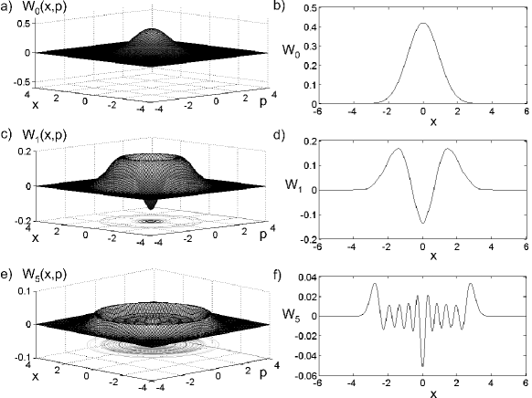
Figure 4: Wigner function representations of the a) 0-click, c) 1-click, and e) 5-clicks measurement outcomes of our eight-bin time-multiplexed detector. A cross-section of each Wigner function is shown in b), d), and f), respectively. The Wigner functions are derived from a theoretical model of the POVMs of our eight-bin time-multiplexed (TMD) detector.

The Wigner function $W_{\gamma}$ is calculated in the standard way from the POVM element $\hat{O}_{\gamma}$ Wigner (1932):

$$W_{\gamma}(x,p)=\frac{1}{\pi\hbar}\int_{-\infty}^{\infty}dy\,\langle x-y|\hat{O}_{\gamma}|x+y\rangle e^{2ipy/\hbar}.$$ (26)

Since the measurement operators $\{\hat{O}_{\gamma}\}$ do not have unit trace, this detector Wigner function is not normalized,

$$\int_{-\infty}^{\infty}dx\,\int_{-\infty}^{\infty}dpW_{\gamma}(x,p)<1,$$ (27)

and its marginals should not be interpreted as probability distributions. Nonetheless, it retains some appealing features. For example, the probability of measurement outcome $\gamma$ is,

$$p_{\gamma}=Tr(\hat{\rho}\hat{O}_{\gamma})=\int_{-\infty}^{\infty}dx\,\int_{-\infty}^{\infty}dpW(x,p)W_{\gamma}(x,p),~{}$$ (28)

where $W$ is the standard Wigner function of the input state $\hat{\rho}.$ Thus one can visualize the measurement as the overlap of the two Wigner functions.

We plot the Wigner functions of the theoretical measurement operators of the TMD in Figure 4. The TMD has no phase sensitivity and so the Wigner function for each measurement operator is rotationally symmetric around a vertical axis through the origin. Thus, on the right of Figure 4 we also present a cross-section of each Wigner function to show its form more clearly. The Wigner functions are found from the TMD POVM that was derived earlier, assuming a loss of 48%. We show three of the nine measurement operators, namely 0-click, 1-click and 5-click (in the figure, these are $W_{0}(x,p),$ $W_{1}(x,p)$ and, $W_{5}(x,p)$, respectively). Remarkably, the 0-click and 1-click Wigner functions look very similar to their state counterparts, the vacuum state and single-photon state. This is despite the fact that there are contributions from all incoming photon numbers to both (i.e., four incoming photons might all be lost and thus result in a 0-click event, or two incoming photons might end up in the same time bin and thus result in 1-click). The 0-click Wigner function has a Gaussian profile similar to the vacuum Wigner function, whereas the 1-click event goes negative at the origin just as the single-photon state does.

The Wigner functions for higher click numbers quickly diverge from their photonic equivalents though. The 5-click Wigner function is significantly different from the five photon Wigner function; the former has nine radial nodes, whereas the latter has five (the number of nodes equals the photon number for Fock states). Since there are only eight bins, there is a sizeable probability that six or seven incoming photons entered only five bins in total. Consequently, there will be significant contributions to the 5-click Wigner function from these higher photon numbers, distorting it from the ideal five photon Wigner function. In contrast, the probability that two or three incoming photons entered only one bin is relatively small, which explains why 1-click Wigner function contains much less distortion.

VI Conclusion

We have detailed a proposal for performing detector tomography on two detectors operating in the Fock space. The proposed testbed generates a sequence of calibrated weak coherent states against which to reference a detector. We have shown that these coherent states form a tomographically complete set for the two detectors, and thus, a tomographic reconstruction of all the POVM elements should be possible. In the near future, we plan to perform detector tomography on these two detectors. However, we envision that a reconstruction of the POVM elements in the high-dimensional photon number space will present substantial computational challenges. The reconstruction will also have to deal with noise and uncertainty in the input states. This is usually not considered in state tomography, where the measurements are considered to be close to ideal.

With the demonstration of detector tomography, experimentalists will have general procedures for characterizing all the parts of a general quantum device: the input states, the quantum circuit, and, now, the measurement. We expect this detector tomography to be particularly useful for devices that depend on generalized measurements for optimal functioning, such as state or process discriminators (i.e., unambiguous state discrimination Peres (1988); Mohseni et al. (2004)). Detector tomography should also be useful for devices where measurement drives logic such as in cluster-state computing or linear optics quantum computing.

References

- Smithey et al. (1993) D. T. Smithey, M. Beck, M. G. Raymer, and A. Faridani, Phys. Rev. Lett. 70, 1244 (1993).
- Dunn et al. (1995) T. J. Dunn, I. A. Walmsley, and S. Mukamel, Phys. Rev. Lett. 74, 884 (1995).
- White et al. (1999) A. G. White, D. F. V. James, P. H. Eberhard, and P. G. Kwiat, Phys. Rev. Lett. 83, 3103 (1999).
- Childs et al. (2001) A. M. Childs, I. L. Chuang, and D. W. Leung, PRA 64, 012314 (2001).
- Mitchell et al. (2003) M. W. Mitchell, C. W. Ellenor, S. Schneider, and A. M. Steinberg, Phys. Rev. Lett. 91, 120402 (2003).
- White et al. (2001) A. G. White, D. F. V. James, W. J. Munro, and P. G. Kwiat, Phys. Rev. A 65, 012301 (2001).
- Lvovsky et al. (2001) A. I. Lvovsky, H. Hansen, O. Aichele, T. Benson, M. J., and S. Schiller, Phys. Rev. Lett. 87, 050402 (2001).
- O’Brien et al. (2004) J. L. O’Brien, G. J. Pryde, A. Gilchrist, D. F. V. James, N. K. Langford, T. C. Ralph, and A. G. White, Phys. Rev. Lett. 93, 080502 (2004).
- Myrskog et al. (2005) S. H. Myrskog, J. K. Fox, M. W. Mitchell, and A. M. Steinberg, Phys. Rev. A 72, 013615 (2005).
- Luis and Sánchez-Soto (1999) A. Luis and L. L. Sánchez-Soto, Phys. Rev. Lett. 83, 3573 (1999).
- Raussendorf and Briegel (2001) R. Raussendorf and H. J. Briegel, Phys. Rev. Lett. 86, 5188 (2001).
- Resch et al. (2007a) K. J. Resch, K. L. Pregnell, R. Prevedel, A. Gilchrist, G. J. Pryde, J. L. O’Brien, and A. G. White, Phys. Rev. Lett. 98, 223601 (2007a).
- Resch et al. (2007b) K. J. Resch, P. Puvanathasan, J. S. Lundeen, M. W. Mitchell, and K. Bizheva, Optics Express 15, 8797 (2007b),
- Fiurasek (2001) J. Fiurasek, Phys. Rev. A 64, 024102 (2001).
- D’Ariano et al. (2004) G. M. D’Ariano, L. Maccone, and P. L. Presti, Phys. Rev. Lett. 93, 250407 (2004).
- D’Ariano and Perinotti (2007) G. M. D’Ariano and P. Perinotti, Phys. Rev. Lett. 98, 020403 (2007).
- Peres (1990) A. Peres, Found. Phys. 12, 1441 (1990).
- Coldenstrodt-Ronge and Silberhorn (2007) H. B. Coldenstrodt-Ronge and C. Silberhorn, J. Phys. B 40, 3909 (2007).
- Paul et al. (1996) H. Paul, P. Torma, T. Kiss, and I. Jex, Phys. Rev. Lett. 76, 2464 (1996).
- Kok and Braunstein (2001) P. Kok and S. L. Braunstein, Phys. Rev. A 6303 (2001).
- Banaszek and Walmsley (2003) K. Banaszek and I. A. Walmsley, Optics Letters 28, 52 (2003).
- Achilles et al. (2003) D. Achilles, C. Silberhorn, C. Sliwa, K. Banaszek, and I. A. Walmsley, Optics Letters 28, 2387 (2003).
- Fitch et al. (2003) M. J. Fitch, B. C. Jacobs, T. B. Pittman, and J. D. Franson, Phys. Rev. A 68, 043814 (2003).
- Silberhorn et al. (2004) C. Silberhorn, D. Achilles, A. B. U’Ren, K. Banaszek, and I. A. Walmsley, in In Proceedings of the Seventh International Conference on Quantum Communication, Measurement and Computing QCMC 2004, held July 25-29, 2004 in Glasgow, UK (2004).
- Achilles et al. (2006) D. Achilles, C. Silberhorn, and I. A. Walmsley, Phys. Rev. Lett. 97, 043602 (2006).
- Achilles et al. (2004) D. Achilles, C. Silberhorn, C. Sliwa, K. Banaszek, I. A. Walmsley, M. J. Fitch, B. C. Jacobs, T. B. Pittman, and J. D. Franson, J. Mod. Opt. 51, 1499 (2004).
- Leonhardt (1997) U. Leonhardt, Measuring the Quantum State of Light (Cambridge University Press, 1997).
- Boyd and Vandenberghe (2004) S. Boyd and L. Vandenberghe, Convex Optimization (Cambridge University Press, 2004).
- Raymer and Beck (2004) M. G. Raymer and M. Beck, Quantum State Estimation (Springer, 2004), pp. 235–295.
- Lanyon et al. (2007) B. P. Lanyon, T. J. Weinhold, N. K. Langford, M. Barbieri, D. F. V. James, A. Gilchrist, and A. G. White, Phys. Rev. Lett. 99, 250505 (2007).
- Rhode (2005) P. P. Rhode, quant-ph/0411114 (2005).
- Wigner (1932) E. Wigner, Phys. Rev. 40, 749 (1932).
- Peres (1988) A. Peres, Physics Letters A 128, 19 (1988).
- Mohseni et al. (2004) M. Mohseni, A. M. Steinberg, and J. A. Bergou, Phys. Rev. Lett. 93, 200403 (2004).