Conserving Quasiparticle Calculations for Small Metal Clusters

Abstract

A novel approach for GW-based calculations of quasiparticle properties for finite systems is presented, in which the screened interaction is obtained directly from a linear response calculation of the density-density correlation function. The conserving nature of our results is shown by explicit evaluation of the $f$-sum rule. As an application, energy renormalizations and level broadenings are calculated for the closed-shell Na${}_{9}^{+}$ and Na${}_{21}^{+}$ clusters, as well as for Na₄. Pronounced improvements of conserving approximations to RPA-level results are obtained.

I Introduction

The GW approximation for the self-energy Hedinfirst is used widely and with considerable success OnidaReiningRubio ; Gunnarsson ; EcheniqueAryasetiawan ; Rohlfing2 ; HolmBarth ; SchoeneEguiluz ; Faleev ; Kotliar in Green’s function based methods to compute bulk and surface electronic band structures and lifetimes for a variety of metals and semiconductors. Within this approach, the self-energy $\Sigma=i\hbar GW$, computed from the single-particle Green’s function $G$ and the dynamically screened interaction $W$, is the fundamental quantity that describes the influence of electronic correlations on the single-particle band structure. Despite the remarkable success of the standard GW theory, which constructs $W$ from the dielectric function in the random-phase approximation (GW-RPA) OnidaReiningRubio ; Gunnarsson ; EcheniqueAryasetiawan ; Rohlfing2 , it is still debated how self-consistency should be implemented and whether it is actually needed HolmBarth ; SchoeneEguiluz ; Faleev ; Kotliar ; Ku . Furthermore, there have been efforts to go beyond the GW approximation by introducing vertex corrections MahanSernelius ; Schindlmayr1998vertex ; TammeSchepe ; Takada .

In this paper, we present a general approach for GW calculations of quasiparticle (QP) properties, in which an accurate screened Coulomb potential is calculated based on consistency requirements between the single-particle Green’s function (determined by the self-energy) and the screened potential (determined by the density-density correlation function). Such an approach is particularly well suited for metal clusters, which combine features of finite systems with those of extended ones BennemannPRL ; EcheniqueNano ; YaroslavHubner . In clusters, both correlations between electrons in localized states and collective excitations influence the band structure and therefore must be taken into account. Usual approximations common to GW calculations for the limiting cases of small atomic systems and extended systems encounter potential problems for clusters. For instance, it is difficult to describe screening effects in a quantum chemistry approach based on perturbation theory starting from the Hartree-Fock (HF) Hamiltonian. On the other hand, the influence of electronic correlations cannot be captured by mean-field screening models such as simple plasmon-pole or static approximations. Therefore it is important to compute the dynamically screened Coulomb potential, which contains two-particle correlations, as accurately as possible in the course of the GW calculation.

The calculation of the screened Coulomb potential is the main difference of our approach from standard GW-RPA and its selectively improved versions. The motivation for this change in approach is that $W$ as computed in the GW-RPA is an auxiliary quantity, which lacks some of the properties of a physical screened potential HolmBarth . To be more specific, GW-RPA does not obey the charge/current conservation law as it applies to the density-density correlation function, unless the screened potential $W$ is calculated from single-particle Green’s function in the Hartree approximation Baym-Kadanoff:PR . This approximation, however, is clearly not good enough for clusters. Using Green’s functions determined self-consistently instead of the Hartree Green’s function seems to be a straightforward improvement for the calculation of $W$, but it leads to a violation of the $f$-sum rule Szymansky , and therefore is in conflict with our goal of improving the quality of the screened Coulomb potential.

To obtain a screened Coulomb potential that does not violate sum rules, we choose the self-energy first, and obtain the consistent screened potential (including vertex corrections) by the physical constraint that the polarization function (or density-density correlation function) fulfils charge/current conservation StrinatiMattauschHanke ; Baym-Kadanoff:PR . This can be achieved by determining the density-density correlation function as a functional derivative of the Green’s function with respect to an external potential Baym-Kadanoff:PR ; Kwong-Bonitz . Using the functional derivative technique, the concept of $\Phi$-derivability is not explicitly needed BaymPR , if one starts from conserving Green’s functions, as is the case in our calculations. Since we cannot exactly compute the functional derivative of a Green’s function with respect to an external potential, we obtain an approximate functional derivative by solving a linearized quantum-kinetic equation for the one-particle Green’s function in the presence of a weak external potential with a generalized QP ansatz. Particle-number conservation on the two-particle level is explicitly checked by evaluating the $f$-sum rule.

Our GW approach for finite systems starts from the HF single-particle energies and wavefunctions, because the correlations described by the GW self-energy can be naturally divided into a HF and a correlation part. The HF contribution is expected to be important in finite systems, and our approach directly allows one to introduce approximations in the correlation part, while keeping the HF contribution unchanged.

At this point a few remarks are in order to relate our approach to other strategies to perform GW calculations. Written in an abstract form Hedin-Lundqvist , the interacting Green’s function is determined by the Dyson equation

$$G=G_{0}+G_{0}\Sigma G,$$ (1)

where $G_{0}$ denotes the non-interacting Green’s function. The quality of a Green’s function calculation is controlled by the self energy

$$\Sigma=i\hbar GW\Gamma$$ (2)

which is given in terms of the screened potential

$$W=v+vPW,$$ (3)

with the bare Coulomb potential $v$ and the irreducible polarization function

$$P=-i\hbar GG\Gamma.$$ (4)

The irreducible polarization function can, in principle, be computed from the (two-particle) density-density correlation function $\chi$, which is identical to the reducible polarization function. The expressions (2) and (4) contain the exact vertex function $\Gamma$

$$\Gamma=1+\frac{\delta\Sigma}{\delta G}GG\Gamma,$$ (5)

which, in turn, depends on the exact self energy $\Sigma$. For approximations to the coupled set of equations (1)–(5), the vertex insertions for self energy and polarization function need not agree Szymansky ; StrinatiMattauschHanke . An important question for the design of a calculational procedure is therefore the selection of approximations for the vertex corrections entering Eqs. (2) and (4) together with the choice of which of the quantities are to be updated in a computational self-consistency cycle. For this choice, no criteria exist in the framework of formal Green’s functions theory StrinatiMattauschHanke , so that, for instance, the calculational procedure can be determined by optimization for a particular system and/or the physical quantities of interest Almbladh . Or the vertex corrections and the self-consistency procedure are chosen using a “best $G$, best $W$” philosophy, which aims at an optimization of the two quantities separately, although it has been shown that this approach should be avoided DelSolePRB . A different approach to choosing the vertex corrections is based on diagrammatic arguments and has been applied to extended systems MahanSernelius ; Schindlmayr1998vertex and finite systems ShirleyMartin . The latter reference uses, for instance, the same exchange vertex both in the self energy and the polarization function. Using diagrammatic arguments, extra care needs to be taken in order to avoid double counting of diagrams in the expressions for the self energy and the polarization.

Instead of using any of the above mentioned techniques to design suitable approximations, one can also use general criteria derived from physical conservation laws or invariance principles. Such an approach has been used for transport calculations Baym-Kadanoff:PR and electronic structure calculations StrinatiMattauschHanke ; Szymansky ; Takada . Since the conservation laws imply important consistency conditions for the one and two-particle correlation functions Baym-Kadanoff:PR ; StrinatiMattauschHanke , they prevent a choice of the vertex contributions that optimizes, say, the one-particle properties at the cost of the two-particle correlation functions. The choice of vertex corrections, which are inconsistent in the sense that they do not obey the charge-current conservation law, may be suitable for a particular calculation, but such a choice is more likely to encounter problems with calculations where both the single-particle quantities (i.e., $G$ and $\Sigma$) and the two-particle quantities (i.e., $W$ and $P$) are intimately connected. The question of consistency between the different “ingredients” for the calculation also arises if one uses, for instance, density-functional based single-particle states as input in GW calculations, which are then used as input to Bethe-Salpeter equation calculations OnidaReiningRubio .

The manuscript is organized as follows. The theoretical approach is described in Section II. Section III presents, as an application of the general method, results on the renormalized single-particle energies and level broadenings in Na clusters of different sizes. The $f$-sum rule for finite systems is derived in Appendix A. To facilitate the comparison of our approach to existing calculations based on the Bethe-Salpeter equation, a comparison between the two is presented in Appendix B. Appendix B also demonstrates the relation of our quantum-kinetic calculation in Sec. II with the work of Baym and Kadanoff Baym-Kadanoff:PR .

II Theory

II.1 Equilibrium relations

We start by introducing our notations and by presenting the necessary equations for the equilibrium Green’s functions formalism for finite systems that is used to formulate the GW theory. For the calculation of the one-particle Green’s function from the dynamically screened potential we use the GW self-energy

$$\Sigma(1,2)=i\hbar G(1,2)W(2,1),$$ (6)

where $1=(\mathbf{r}_{1},\sigma_{1},t_{1})$ denotes the space, spin and time variable. The spatial dependence of the functions is expanded in a basis of HF eigenfunctions $\{\varphi_{n}({\mathbf{r}})\}$, where $n$ labels the HF spin orbital. For single-particle quantities such as $G$ and $\Sigma$, we employ the matrix notation

$$G_{n_{1}n_{2}}(t_{1},t_{2})=\sum_{\sigma_{1}\sigma_{2}}\int\varphi^{*}_{n_{1}}({\mathbf{r}}_{1})G(1,2)\varphi_{n_{2}}({\mathbf{r}}_{2}){\mathrm{d}}^{3}r_{1}{\mathrm{d}}^{3}r_{2},$$ (7)

while for two-particle quantities, such as the bare ($v$) or the screened ($W$) Coulomb potentials, we use

$$\langle n_{1}n_{2}|W(t_{1},t_{2})|n_{3}n_{4}\rangle=\sum_{\sigma_{1}\dots\sigma_{4}}\int\varphi^{*}_{n_{1}}({\mathbf{r}}_{1})\varphi^{*}_{n_{2}}({\mathbf{r}}_{2})W(1,2)\varphi_{n_{3}}({\mathbf{r}}_{1})\varphi_{n_{4}}({\mathbf{r}}_{2}){\mathrm{d}}^{3}r_{1}{\mathrm{d}}^{3}r_{2}.$$ (8)

The Dyson equation for the equilibrium ($T=0\,\mathrm{K}$) retarded Green’s function Hedin-Lundqvist

$$\sum_{n_{2}}\left[\hbar(\omega+i\gamma)\delta_{n_{1}n_{2}}-\Sigma^{\mathrm{HF}}_{n_{1}n_{2}}-\Sigma^{\mathrm{corr}}_{n_{1}n_{2}}(\omega)\right]G^{\mathrm{r}}_{n_{2}n_{3}}(\omega)=\delta_{n_{1}n_{3}}$$ (9)

can be written in a form which explicitly displays the static HF and dynamic correlation contributions to the retarded self-energy. The HF self energy

$$\Sigma^{\mathrm{HF}}_{n_{1}n_{2}}=\sum_{n_{3}n_{4}}\bigl{[}\langle n_{1}n_{3}|v|n_{2}n_{4}\rangle-\langle n_{1}n_{2}|v|n_{3}n_{4}\rangle\bigr{]}f_{n_{3}n_{4}}$$ (10)

is determined by the direct and exchange Coulomb matrix elements as well as the one-particle distribution functions

$$f_{n_{1}n_{2}}=-i\hbar\int\frac{d\omega}{2\pi}G^{<}_{n_{1}n_{2}}(\omega).$$ (11)

The correlation contribution to the retarded self-energy $\Sigma^{\mathrm{corr}}(\omega)=\Sigma^{\mathrm{r}}(\omega)-\Sigma^{\mathrm{HF}}$ is connected to the lesser and the greater components by the identity

$$\mathrm{Im}\Sigma^{\mathrm{corr}}_{n_{1}n_{1}}(\omega)=\frac{1}{2i}\left(\Sigma^{>}_{n_{1}n_{1}}(\omega)-\Sigma^{<}_{n_{1}n_{1}}(\omega)\right).$$ (12)

In the GW approximation and in a discrete basis function representation, they read

$$\Sigma^{\gtrless}_{n_{1}n_{1}}(\omega)=i\hbar\sum_{n_{2}}\int\frac{{\mathrm{d}}\omega^{\prime}}{2\pi}G^{\gtrless}_{n_{2}n_{2}}(\omega+\omega^{\prime})\langle n_{1}n_{1}|W^{\lessgtr}(\omega^{\prime})|n_{2}n_{2}\rangle.$$ (13)

We now need to relate the $>$ and $<$ components of $G$ and $W$ to the retarded functions. For this, we use the fermionic Kubo-Martin-Schwinger conditions Kadanoff-Baym:Book

$$G^{<}(\omega)= -2\,in_{\mathrm{F}}(\omega)\,\mathrm{Im}G^{\mathrm{r}}(\omega)$$ (14)

$$G^{>}(\omega)= -2\,i\big{[}n_{\mathrm{F}}(\omega)-1\big{]}\,\mathrm{Im}G^{\mathrm{r}}(\omega),$$ (15)

with the Fermi function $n_{\mathrm{F}}(\omega)=[\exp(\beta\hbar\omega)+1]^{-1}$, where $\beta=1/k_{B}T$. In the $T=0$ K limit, $n_{\mathrm{F}}(\omega)=\Theta(\epsilon_{\mathrm{F}}-\hbar\omega)$, with the step function $\Theta$ and $\epsilon_{\mathrm{F}}$ the Fermi energy. Then one obtains for Eq. (11), which enters the HF self energy,

$$f_{n_{1}n_{2}}=\frac{\hbar}{\pi}\int_{-\infty}^{\epsilon_{\mathrm{F}}}d\omega\mathrm{Im}G^{\mathrm{r}}_{n_{1}n_{2}}(\omega).$$ (16)

For the screened Coulomb potential, which is related to a two-particle correlation function, the bosonic Kubo-Martin-Schwinger conditions read Kuznetsov

$$W^{<}(\omega)= \,2\,in_{\mathrm{B}}(\omega)\,\mathrm{Im}W^{\mathrm{r}}(\omega)$$ (17)

$$W^{>}(\omega)= \,2\,i\big{(}n_{\mathrm{B}}(\omega)+1\big{)}\,\mathrm{Im}W^{\mathrm{r}}(\omega).$$ (18)

In Eq. (17), $n_{\mathrm{B}}(\omega)=[\exp(\beta\hbar\omega)-1]^{-1}$ is the Bose function. In the $T=0$ K limit, $n_{\mathrm{B}}(\omega)=-\Theta(-\hbar\omega)$. Inserting (14) and (17) into (13), we obtain for the self-energies

$$\Sigma^{>}_{n_{1}n_{1}}(\omega) =4i\hbar\sum_{n_{2}}\int\frac{{\mathrm{d}}\omega^{\prime}}{2\pi}n_{\mathrm{B}}(\omega^{\prime})\big{[}n_{\mathrm{F}}(\omega+\omega^{\prime})-1\big{]}\mathrm{Im}G^{\mathrm{r}}_{n_{2}n_{2}}(\omega+\omega^{\prime})\,\mathrm{Im}\langle n_{1}n_{1}|W^{\mathrm{r}}(\omega^{\prime})|n_{2}n_{2}\rangle,$$ (19)

$$\Sigma^{<}_{n_{1}n_{1}}(\omega) =4i\hbar\sum_{n_{2}}\int\frac{{\mathrm{d}}\omega^{\prime}}{2\pi}\big{[}n_{\mathrm{B}}(\omega^{\prime})+1\big{]}n_{\mathrm{F}}(\omega+\omega^{\prime})\mathrm{Im}G^{\mathrm{r}}_{n_{2}n_{2}}(\omega+\omega^{\prime})\,\mathrm{Im}\langle n_{1}n_{1}|W^{\mathrm{r}}(\omega^{\prime})|n_{2}n_{2}\rangle.$$ (20)

From Eqs. (12) and (19), a Montroll-Ward expression KraeftPREetal for the imaginary part of the correlated (retarded) self-energy

$$\mathrm{Im}\Sigma^{\mathrm{corr}}_{n_{1}n_{1}}(\omega)=\hbar\sum_{n_{2}}\int\frac{{\mathrm{d}}\omega^{\prime}}{\pi}\left[n_{\mathrm{B}}(\omega^{\prime})+n_{\mathrm{F}}(\omega+\omega^{\prime})\right]\mathrm{Im}G^{\mathrm{r}}_{n_{2}n_{2}}(\omega+\omega^{\prime})\,\mathrm{Im}\langle n_{1}n_{1}|W^{\mathrm{r}}(\omega^{\prime})|n_{2}n_{2}\rangle$$ (21)

can be derived. The real part of $\Sigma^{\mathrm{corr}}(\omega)$ is calculated from a Kramers-Kronig transformation of Eq. (21).

The computation of $\Sigma^{\mathrm{corr}}$ is closely linked with the screened Coulomb potential, $W^{\mathrm{r}}$ or, equivalently, the inverse dielectric function. They can be constructed from the retarded density-density correlation function $\chi^{\mathrm{r}}$ using

$$W^{\mathrm{r}}(1,2)=\int{\mathrm{d}}3\varepsilon^{-1}(1,3)\,v(3,2)=v(1,2)+\int{\mathrm{d}}3{\mathrm{d}}4\,v(1,3)\chi^{\mathrm{r}}(3,4)\,v(4,2),$$ (22)

where $\int d3=\int d^{3}r_{3}dt_{3}$. The correlation function $\chi^{\mathrm{r}}$ is also the retarded density-response function Baym-Kadanoff:PR ; Hedin-Lundqvist ; Kwong-Bonitz with respect to a weak external perturbation $U$, i.e.,

$$\chi^{\mathrm{r}}(1,2)=\left.\frac{\delta\langle\rho(1)\rangle}{\delta U(2)}\right|_{U=0},$$ (23)

where $\rho(1)=\psi^{{\dagger}}(1)\psi(1)$ is the particle density operator, expressed through the creation and destruction field operators $\psi^{{\dagger}}$ and $\psi$, respectively. The response function in Eq. (23) can therefore be calculated in the framework of nonequilibrium Green’s functions Binder-Koch ; Kremp:Book ; Kwong-Bonitz , using exactly the same GW approximation as employed for the determination of the single-quasiparticle properties. The determination of a dielectric function that is consistent with the GW self-energy is carried out in the next section.

II.2 Quantum kinetics

In our basis function representation, the single-particle density matrix is given in terms of a single-particle nonequilibrium Green’s function

$$i\hbar G_{n_{2}n_{1}}^{<}(t,t)=-\langle\rho_{n_{1}n_{2}}(t)\rangle=-\langle c^{{\dagger}}_{n_{1}}(t)c_{n_{2}}(t)\rangle,$$ (24)

where $c^{{\dagger}}_{n}$ and $c_{n}$ are the creation and the annihilation operators of particles in the molecular orbital $n$, respectively.

In the following, we relate the determination of $\chi^{\mathrm{r}}$ to a quantum-kinetic calculation of a nonequilibrium Green’s function under the action of a weak external field $U$. For this, we start from the Hamiltonian

$$H= \sum_{n_{1}}T_{n_{1}n_{1}}c^{{\dagger}}_{n_{1}}(t)c_{n_{1}}(t)+\sum_{n_{1}n_{2}}U_{n_{1}n_{2}}(t)c^{{\dagger}}_{n_{1}}(t)c_{n_{2}}(t)$$

$$+\frac{1}{2}\sum_{n_{1}\dots n_{4}}\langle n_{1}n_{2}|v|n_{4}n_{3}\rangle c^{{\dagger}}_{n_{1}}(t)c^{{\dagger}}_{n_{2}}(t)c_{n_{3}}(t)c_{n_{4}}(t),$$ (25)

where $T$ is the kinetic part, which in our case includes the core potential, and $v$ is the bare Coulomb matrix element, with the index structure defined in Eq. (8). With this Hamiltonian, the Green’s function (24) evolves in time according to

$$i\hbar\frac{\partial}{\partial t_{1}}G^{<}_{n_{1}n_{2}}(t_{1},t_{2})=\mbox{} \delta(t_{1}-t_{2})\delta_{n_{1}n_{2}}$$ (26)

$$+T_{n_{1}n_{1}}(t_{1})G^{<}_{n_{1}n_{2}}(t_{1},t_{2})+\sum_{n_{3}}U_{n_{1}n_{3}}(t_{1})G^{<}_{n_{3}n_{2}}(t_{1},t_{2})$$

$$+\sum_{n_{3}}\int\mathrm{d}t_{3}\big{(}\Sigma^{\mathrm{r}}_{n_{1}n_{3}}(t_{1},t_{3})G^{<}_{n_{3}n_{2}}(t_{3},t_{2})+\Sigma^{<}_{n_{1}n_{3}}(t_{1},t_{3})G^{\mathrm{a}}_{n_{3}n_{2}}(t_{3},t_{2})\big{)}.$$

There is also the adjoint equation, corresponding to the derivative with respect to $t_{2}$.

We next compile the relations between $G$, $W$ and $\Sigma$ that generalize the equilibrium functions (12)–(19) to dynamical quantities, and which are needed for the evaluation of Eq. (26)

$$G^{\mathrm{r}}(t_{1},t_{2})=\mbox{} \Theta(t_{1}-t_{2})\big{(}G^{>}(t_{1},t_{2})-G^{<}(t_{1},t_{2})\big{)}$$ (27)

$$W^{\mathrm{r}}(t_{1},t_{2})=\mbox{} v\,\delta(t_{1}-t_{2})+\Theta(t_{1}-t_{2})\big{(}W^{>}(t_{1},t_{2})-W^{<}(t_{1},t_{2})\big{)}$$ (28)

$$\Sigma^{\mathrm{r}}(t_{1},t_{2})=\mbox{} \Sigma^{\mathrm{HF}}(t_{1})\delta(t_{1}-t_{2})+\Theta(t_{1}-t_{2})\big{(}\Sigma^{>}(t_{1},t_{2})-\Sigma^{<}(t_{1},t_{2})\big{)}.$$ (29)

The instantaneous HF contribution is given by:

$$\Sigma^{\mathrm{HF}}_{n_{1}n_{2}}(t_{1})=-i\hbar\sum_{n_{3}n_{4}}\langle n_{1}n_{3}|v|n_{2}n_{4}\rangle G^{<}_{n_{3}n_{4}}(t_{1},t_{1})+i\hbar\sum_{n_{3}n_{4}}\langle n_{1}n_{2}|v|n_{3}n_{4}\rangle G^{<}_{n_{3}n_{4}}(t_{1},t_{1}).$$ (30)

Finally, for $\Sigma^{\gtrless}(t_{1},t_{2})$ we use the GW form

$$\Sigma_{n_{1}n_{2}}^{\gtrless}(t_{1},t_{2})=i\hbar\sum_{n_{3}n_{4}}G^{\gtrless}_{n_{3}n_{4}}(t_{1},t_{2})\langle n_{1}n_{2}|W^{\lessgtr}(t_{2},t_{1})|n_{3}n_{4}\rangle.$$ (31)

The above equations completely determine the system’s response to the external potential in the GW approximation if they are supplemented by the dynamical equations for another Green’s function, say, for the retarded Green’s function $G^{\mathrm{r}}(t_{1},t_{2})$. In this scheme, both $G^{<}$ and $G^{\mathrm{r}}$ depend on two time arguments, and the retarded function describes the changes of the spectral properties of the systems during the time evolution. An implementation of these two-time equations for the electron gas was carried out in Ref. Kwong-Bonitz . In this case, the numerical calculation is run starting from non-interacting Green’s functions without external field for some time to obtain the interacting Green’s functions, which are then disturbed by the field. The dynamics under the influence of the weak driving field then allows one to numerically calculate the functional derivative, which determines the dielectric function via Eq. (23). Since one can use the same self-energy, say, in the GW approximation for both the kinetic and the spectral Green’s function, the dielectric function determined in this way is consistent by construction with the single-particle Green’s function determined from the same self-energy.

Equation (26) for the dynamical Green’s functions depending on two real time arguments is an extremely complex integro-differential equations, whose solution is possible only for small or homogeneous systems theDuchGuy . For systems of intermediate size, our aim is to develop a flexible approximate numerical scheme which works only with Green’s functions depending on a single time argument. To this end, one can introduce approximations, so that the resulting equations depend only on $G^{\mathrm{r}}(t_{1}-t_{2})$, i.e., the equilibrium retarded Green’s function, whose Fourier transformation $G^{\mathrm{r}}(\omega)$ has a simple physical interpretation, instead of $G^{\mathrm{r}}(t_{1},t_{2})$. An important consequence of this approximation is that the equilibrium $G^{\mathrm{r}}(t_{1}-t_{2})$ does not need to be calculated together with the dynamical Eq. (26). Rather, the response of the system described by Eq. (26) now becomes implicitly dependent on $G^{\mathrm{r}}(\omega)$. Of course, the density-response function determines the screening properties, so that $G^{\mathrm{r}}(\omega)$ depends on the response calculation. This interdependence introduces the possibility of a self-consistent numerical procedure, in which one or both of these quantities are updated and recalculated during the self-consistency cycle.

In this paper we concentrate on setting up the numerical procedure for a consistent GW calculation in the spirit of Hedin’s original GW treatment as a “one-shot” self-energy correction to the HF ground state. We do not intend to study the issue of self-consistency here. We begin by writing down the Green’s functions of the finite system in the HF approximation

$$\sum_{n_{2}}\left[\hbar(\omega+i\gamma)\delta_{n_{1}n_{2}}-\Sigma^{\mathrm{HF}}_{n_{1}n_{2}}\right]G^{\mathrm{r\ (HF)}}_{n_{2}n_{3}}(\omega)=\delta_{n_{1}n_{3}}.$$ (32)

Using HF spin orbitals as single-particle quantum numbers, this GF becomes diagonal

$$G^{\mathrm{r\ (HF)}}_{n_{1}n_{2}}(\omega)=\frac{1}{\hbar(\omega+i\gamma)-\epsilon^{\mathrm{HF}}_{n_{1}}}\ \delta_{n_{1}n_{2}}.$$ (33)

In equilibrium, this corresponds also to a diagonal kinetic Green’s function

$$G^{<\ \mathrm{(HF)}}_{n_{1}n_{2}}(\omega)=-2\,in_{\mathrm{F}}(\omega)\,\mathrm{Im}G^{\mathrm{r\ (HF)}}_{n_{1}n_{1}}(\omega)\ \delta_{n_{1}n_{2}}.$$ (34)

In the limit $\gamma\to 0$, the equilibrium single-particle correlation functions are simply given by

$$G^{<\ \mathrm{(HF)}}_{n_{1}n_{2}}(\omega) =2\pi if_{n_{1}n_{2}}^{\mathrm{(HF)}}\delta(\hbar\omega-\epsilon^{\mathrm{HF}}_{n_{1}})$$ (35)

$$f_{n_{1}n_{2}}^{\mathrm{(HF)}} \mbox{}=n_{\mathrm{F}}(\epsilon^{\mathrm{HF}}_{n_{1}})\,\delta_{n_{1}n_{2}},$$ (36)

Employing Eq. (35) as a description of the HF ground state, we determine the dielectric function via Eq. (23). To do this, we need several additional steps and an approximation for the two-time kinetic Green’s function. We first note that, by definition of the functional derivative, we only need to be interested in the linear response to a weak time-dependent perturbing potential $U$. To first order in the weak perturbation, only density fluctuations, i.e., averages of the form $\langle\rho_{n_{1}n_{2}}(t)\rangle$ with $n_{1}\neq n_{2}$, are driven away from their equilibrium value (36), while the level occupations $\langle\rho_{n_{1}n_{1}}\rangle$ remain equal to $f_{n_{1}n_{1}}^{\mathrm{(HF)}}=n_{\mathrm{F}}(\epsilon^{\mathrm{HF}}_{n_{1}})$ for all times. In the numerical calculations, we take $\epsilon_{\mathrm{F}}$ to be in the middle of the gap between the highest occupied and lowest unoccupied molecular orbital.

Transcribing this back into the language of Green’s functions using Eq. (24), we need to calculate the Green’s functions off-diagonal in the level indices $i\hbar G^{<}_{n_{1}n_{2}}(t,t)$, with $n_{1}\neq n_{2}$. The quantum kinetic equation for these quantities is derived by subtracting Eq. (26) and the adjoint equation, making the substitution $t=(t_{1}+t_{2})/2$ and $\tau=t_{1}-t_{2}$ and finally considering the equal-time limit $t_{1}=t_{2}=t$, $\tau=0$:

$$(i\hbar\frac{\partial}{\partial t}-\epsilon_{\alpha}^{\mathrm{HF}})G^{<}_{\alpha}(t)+n_{\alpha}\Omega^{\mathrm{eff}}_{\alpha}(t)=S_{\alpha}(t).$$ (37)

Here, $\alpha=(n_{1},n_{2})$ is a pair-state index for the off-diagonal Green’s function, $\epsilon_{\alpha}^{\mathrm{HF}}=\epsilon_{n_{1}}^{\mathrm{HF}}-\epsilon_{n_{2}}^{\mathrm{HF}}$ the energy difference between two levels, and $n_{\alpha}=n_{\mathrm{F}}(\epsilon_{n_{1}})-n_{\mathrm{F}}(\epsilon_{n_{2}})$ is the difference in level distribution between the two spin-orbitals of the pair state. The latter quantity is sometimes referred to as the Pauli-blocking factor. The generalized driving term

$$\hbar\Omega^{\mathrm{eff}}_{\alpha}(t)=iU_{\alpha}(t)+\hbar\sum_{\beta}(v^{\mathrm{dir}}_{\alpha\beta}-v^{\mathrm{exc}}_{\alpha\beta})G^{<}_{\beta}(t)$$ (38)

contains Coulomb enhancement contributions involving direct and exchange matrix elements $v^{\mathrm{dir}}$ and $v^{\mathrm{exc}}$

$$v_{\alpha\beta}^{\mathrm{dir}}=v_{(n_{1}n_{2})(n_{3}n_{4})}^{\mathrm{dir}}=\langle n_{1}n_{3}|v|n_{2}n_{4}\rangle,$$ (39)

$$v_{\alpha\beta}^{\mathrm{exc}}=v_{(n_{1}n_{2})(n_{3}n_{4})}^{\mathrm{exc}}=\langle n_{1}n_{2}|v|n_{3}n_{4}\rangle.$$ (40)

The right hand side of Eq. (37) is the correlation term

$$S_{n_{1}n_{2}}(t)=\sum_{n_{3}}\int_{-\infty}^{t}{\mathrm{d}}\bar{t}\big{[}\Sigma^{>}_{n_{1}n_{3}}(t,\bar{t})G^{<}_{n_{3}n_{2}}(\bar{t},t)+G^{<}_{n_{1}n_{3}}(t,\bar{t})\Sigma^{>}_{n_{3}n_{2}}(\bar{t},t)-(\lessgtr\leftrightarrow\gtrless)\big{]}$$ (41)

that accounts for interaction effects beyond HF. For the self-energies, we use Eq. (31).

The aim of our approach is to reduce the computational complexity of the Green’s functions depending on two time arguments, where kinetic and spectral properties are tied closely together, by splitting the problem into the the determination of the equilibrium $G^{\mathrm{r}}(\omega)$ from the calculation of the density-response function, i.e., $G^{<}(t,t)$ in the presence of an external perturbation. The main approximation involved in this split is that the two-time Green’s functions $G^{<}(t,\bar{t})$, which are contained in the correlation contribution (41) need to be related to the dynamics of the density response, i.e., the time-diagonal Green’s function by virtue of Eq. (24). To this end, we employ a generalized Kadanoff-Baym ansatz in the form JahnkeKiraKoch

$$G^{\gtrless}_{n_{1}n_{2}}(t,\bar{t})=i\hbar G_{n_{1}n_{1}}^{\mathrm{r}}(t-\bar{t})G^{\gtrless}_{n_{1}n_{2}}(\bar{t})-i\hbar G^{\gtrless}_{n_{1}n_{2}}(t)G_{n_{2}n_{2}}^{\mathrm{a}}(t-\bar{t})\ .$$ (42)

For notational simplicity, we write here and in the following $G^{\gtrless}_{n_{1}n_{2}}(t)$ for $G^{\gtrless}_{n_{1}n_{2}}(t,t)$. To evaluate the correlation contribution in the generalized Kadanoff-Baym ansatz, the retarded $G^{\mathrm{r}}$ and advanced $G^{\mathrm{a}}$ Green’s functions, we employ the Hartree-Fock Green’s functions in the time domain:

$$i\hbar G_{n_{1}n_{1}}^{\mathrm{r\ (HF)}}(t-\bar{t}) =\Theta(t-\bar{t})\exp\{-\frac{i}{\hbar}\tilde{\epsilon}_{n_{1}}(t-\bar{t})\}$$ (43)

$$i\hbar G_{n_{2}n_{2}}^{\mathrm{a\ (HF)}}(\bar{t}-t) \mbox{}=-\Theta(t-\bar{t})\exp\{-\frac{i}{\hbar}\tilde{\epsilon}^{*}_{n_{2}}(\bar{t}-t)\}.$$ (44)

A non-zero “background” broadening $\gamma$ ensures the proper behavior of the HF retarded and advanced Green’s functions, and we use the notation $\tilde{\epsilon}_{n}=\epsilon^{\mathrm{HF}}_{n}-i\gamma$ . Then the correlation contribution becomes

$$S_{n_{1}n_{2}}(t)=i\hbar\sum_{n_{3}n_{4}n_{5}}\int_{-\infty}^{t}d\bar{t}\big{[} e^{-\frac{i}{\hbar}(\tilde{\epsilon}_{n_{4}}-\tilde{\epsilon}_{n_{2}}^{*})(t-\bar{t})}\langle n_{1}n_{3}|W^{<}(\bar{t},t)|n_{4}n_{5}\rangle G^{<}_{n_{3}n_{2}}(\bar{t})G^{>}_{n_{4}n_{5}}(\bar{t})$$ (45)

$$+ e^{-\frac{i}{\hbar}(\tilde{\epsilon}_{n_{1}}-\tilde{\epsilon}_{n_{5}}^{*})(t-\bar{t})}\langle n_{3}n_{2}|W^{<}(t,\bar{t})|n_{4}n_{5}\rangle G^{<}_{n_{1}n_{3}}(\bar{t})G^{>}_{n_{4}n_{5}}(\bar{t})$$

$$-(\lessgtr\leftrightarrow\gtrless)\big{]}.$$

Because we wish to determine the linear density response to the weak external perturbation, $S(t)$ is linearized with respect to the off-diagonal $G^{\gtrless}$s that are driven by $U$. In the spirit of linear response, the Green’s functions appearing in one term together with one off-diagonal Green’s function are replaced by the equilibrium relations $G^{<}_{n_{1}n_{1}}=\frac{1}{i\hbar}(1-f_{n_{1}})$ and $G^{>}_{n_{1}n_{1}}=-\frac{1}{i\hbar}f_{n_{1}}$, where we have defined $f_{n_{1}}\equiv f^{\mathrm{(HF)}}_{n_{1}n_{1}}$. To further simplify the equations, note also that $G^{>}_{n_{1}n_{2}}(\bar{t})=G^{<}_{n_{1}n_{2}}(\bar{t})$, with $n_{1}\neq n_{2}$. Equation (45) then becomes

$$S_{n_{1}n_{2}}(t)=\sum_{n_{3}n_{4}n_{5}}\int_{-\infty}^{t}{\mathrm{d}}\bar{t} e^{-\frac{i}{\hbar}(\tilde{\epsilon}_{n_{4}}-\tilde{\epsilon}_{n_{2}}^{*})(t-\bar{t})}$$ (46)

$$\Big{[}\delta_{n_{4}n_{5}} G^{<}_{n_{3}n_{2}}(\bar{t})\Big{(}\langle n_{1}n_{3}|W^{<}(\bar{t},t)|n_{4}n_{5}\rangle(1-f_{n_{4}})+\langle n_{1}n_{3}|W^{>}(\bar{t},t)|n_{4}n_{5}\rangle f_{n_{4}}\Big{)}$$

$$-\delta_{n_{3}n_{2}} G^{<}_{n_{4}n_{5}}(\bar{t})\Big{(}\langle n_{1}n_{3}|W^{<}(\bar{t},t)|n_{4}n_{5}\rangle f_{n_{2}}+\langle n_{1}n_{3}|W^{>}(\bar{t},t)|n_{4}n_{5}\rangle(1-f_{n_{2}})\Big{)}\Big{]}$$

$$+\sum_{n_{3}n_{4}n_{5}}\int_{-\infty}^{t}{\mathrm{d}}\bar{t} e^{-\frac{i}{\hbar}(\tilde{\epsilon}_{n_{1}}-\tilde{\epsilon}_{n_{5}}^{*})(t-\bar{t})}$$

$$\Big{[}\delta_{n_{4}n_{5}} G^{<}_{n_{1}n_{3}}(\bar{t})\Big{(}\langle n_{3}n_{2}|W^{<}(t,\bar{t})|n_{4}n_{5}\rangle(1-f_{n_{4}})+\langle n_{3}n_{2}|W^{>}(t,\bar{t})|n_{4}n_{5}\rangle f_{n_{4}}\Big{)}$$

$$-\delta_{n_{1}n_{3}} G^{<}_{n_{4}n_{5}}(\bar{t})\Big{(}\langle n_{3}n_{2}|W^{<}(t,\bar{t})|n_{4}n_{5}\rangle f_{n_{1}}+\langle n_{3}n_{2}|W^{>}(t,\bar{t})|n_{4}n_{5}\rangle(1-f_{n_{1}})\Big{)}\Big{]}.$$

The equation for $\chi^{\mathrm{r}}$ is obtained by functional differentiation of Eq. (37) with respect to $U(t^{\prime})$ and letting $U\to 0$ afterwards. This is done by replacing everywhere the term $\delta G_{n_{1}n_{2}}^{<}(t)/\delta U_{n_{3}n_{4}}(t^{\prime})$ with $-i\hbar\langle n_{1}n_{2}|\chi^{\mathrm{r}}(t-t^{\prime})|n_{3}n_{4}\rangle$. In the correlation contributions, terms such as $\delta W^{\gtrless}/\delta U$ are consistently neglected, because we assume that the external potential is weak enough as not to cause changes in the screening properties of the system. This is in agreement with current developments in GW theory LouieW0 . The resulting equation can be cast in the form

$$(i\hbar\frac{\partial}{\partial t}-\epsilon_{\alpha}^{\mathrm{HF}})\chi^{\mathrm{r}}_{\alpha\beta}(t,t^{\prime})+n_{\alpha}\Big{(}\delta_{\alpha\beta}+\sum_{\gamma}(v^{\mathrm{dir}}_{\alpha\gamma}-v^{\mathrm{exc}}_{\alpha\gamma})\chi^{\mathrm{r}}_{\gamma\beta}(t,t^{\prime})\Big{)}=\sum_{\gamma}\int_{-\infty}^{t}{\mathrm{d}}\bar{t}\Delta_{\alpha\gamma}(t,\bar{t})\chi_{\gamma\beta}^{\mathrm{r}}(\bar{t},t^{\prime}).$$ (47)

The correlation kernel $\Delta$ reads

$$\Delta_{(n_{1}n_{2})(n_{3}n_{4})}(t,\bar{t})=\int\frac{{\mathrm{d}}\omega^{\prime}}{2\pi}\Big{[}- e^{-\frac{i}{\hbar}(\hbar\omega^{\prime}+\tilde{\epsilon}_{n_{1}}-\tilde{\epsilon}_{n_{4}}^{*})(t-\bar{t})}f_{n_{1}}\langle n_{1}n_{2}|W^{<}(\omega^{\prime})|n_{3}n_{4}\rangle$$ (48)

$$- e^{-\frac{i}{\hbar}(-\hbar\omega^{\prime}+\tilde{\epsilon}_{n_{3}}-\tilde{\epsilon}_{n_{2}}^{*})(t-\bar{t})}f_{n_{2}}\langle n_{1}n_{2}|W^{<}(\omega^{\prime})|n_{3}n_{4}\rangle$$

$$+\sum_{n_{5}}(1-f_{n_{5}})\Big{(}\delta_{n_{1}n_{3}} e^{-\frac{i}{\hbar}(\hbar\omega^{\prime}+\tilde{\epsilon}_{n_{3}}-\tilde{\epsilon}_{n_{5}}^{*})(t-\bar{t})}\langle n_{4}n_{2}|W^{<}(\omega^{\prime})|n_{5}n_{5}\rangle$$

$$+\delta_{n_{2}n_{4}} e^{-\frac{i}{\hbar}(-\hbar\omega^{\prime}+\tilde{\epsilon}_{n_{5}}-\tilde{\epsilon}_{n_{4}}^{*})(t-\bar{t})}\langle n_{1}n_{3}|W^{<}(\omega^{\prime})|n_{5}n_{5}\rangle\Big{)}\Big{]}$$

$$+\Big{[}<\longleftrightarrow>, f\longleftrightarrow(1-f)\Big{]},$$

where the last line indicates additional terms, in which $W^{<}$ is replaced by $W^{>}$, $f$ by $1-f$ and $1-f$ by $f$. The integral over $\omega^{\prime}$ in Eq. (48) comes from the Fourier transformation $W^{\gtrless}(t,\bar{t})=\int\frac{{\mathrm{d}}\omega^{\prime}}{2\pi}e^{-i\omega^{\prime}(t-\bar{t})}W^{\gtrless}(\omega^{\prime})$ of the screened potential.

The particular time-dependence of the correlation contributions in Eq. (47) allows us to perform the Fourier transformation with respect to time and to determine the frequency-dependent $\chi^{\mathrm{r}}$ by

$$(\hbar\omega-\epsilon_{\alpha}^{\mathrm{HF}})\chi^{\mathrm{r}}_{\alpha\beta}(\omega)+n_{\alpha}\Big{(}\delta_{\alpha\beta}+\sum_{\gamma}(v^{\mathrm{dir}}_{\alpha\gamma}-v^{\mathrm{exc}}_{\alpha\gamma})\chi^{\mathrm{r}}_{\gamma\beta}(\omega)\Big{)}=\sum_{\gamma}\Delta_{\alpha\gamma}(\omega)\chi_{\gamma\beta}^{\mathrm{r}}(\omega).$$ (49)

Using

$$\int_{-\infty}^{t}{\mathrm{d}}\bar{t}e^{-\frac{i}{\hbar}(\omega\pm\epsilon+i\gamma)\bar{t}}=\frac{i\hbar e^{-\frac{i}{\hbar}(\omega\pm\epsilon+i\gamma)t}}{\omega\pm\epsilon+i\gamma},$$ (50)

integration over $\bar{t}$ yields for the correlation kernel

$$\qquad\Delta_{(n_{1}n_{2})(n_{3}n_{4})}(\omega)=i\hbar\int\frac{\mathrm{d}\omega^{\prime}}{2\pi}\times$$ (51)

$$\quad\Big{(}\frac{f_{n_{1}}}{\hbar\omega-\hbar\omega^{\prime}-\tilde{\epsilon}_{n_{1}}+\tilde{\epsilon}^{*}_{n_{4}}}\langle n_{1}n_{2}|W^{<}(\omega^{\prime})|n_{3}n_{4}\rangle$$

$$\qquad+\frac{f_{n_{2}}}{\hbar\omega+\hbar\omega^{\prime}-\tilde{\epsilon}_{n_{3}}+\tilde{\epsilon}^{*}_{n_{2}}}\langle n_{1}n_{2}|W^{<}(\omega^{\prime})|n_{3}n_{4}\rangle$$

$$\quad-\sum_{n_{5}}\frac{(1-f_{n_{5}})\delta_{n_{1}n_{3}}}{\hbar\omega-\hbar\omega^{\prime}-\tilde{\epsilon}_{n_{3}}+\tilde{\epsilon}^{*}_{n_{5}}}\langle n_{4}n_{2}|W^{<}(\omega^{\prime})|n_{5}n_{5}\rangle$$

$$\qquad-\sum_{n_{5}}\frac{(1-f_{n_{5}})\delta_{n_{4}n_{2}}}{\hbar\omega+\hbar\omega^{\prime}-\tilde{\epsilon}_{n_{5}}+\tilde{\epsilon}^{*}_{n_{4}}}\langle n_{1}n_{3}|W^{<}(\omega^{\prime})|n_{5}n_{5}\rangle\Big{)}$$

$$\qquad\qquad+\Big{[}\big{(}<\rightarrow>\big{)},\big{(}f\leftrightarrow(1-f)\big{)}\Big{]}.$$

Further, the functions $W^{\gtrless}$ are related to Im$W^{\mathrm{r}}$ through the Kubo-Martin-Schwinger boundary conditions (17). Finally, the retarded screened potential needs to be determined from the density response function via the discrete version of Eq. (22), i.e., by using

$$\langle n_{1}n_{2}|W^{\mathrm{r}}(\omega)|n_{3}n_{4}\rangle=\langle n_{1}n_{2}|v|n_{3}n_{4}\rangle$$ (52)

$$\quad+\sum_{n_{5}\dots n_{8}}\langle n_{1}n_{5}|v|n_{3}n_{7}\rangle\langle n_{5}n_{6}|\chi^{\mathrm{r}}(\omega)|n_{7}n_{8}\rangle\langle n_{2}n_{6}|v|n_{4}n_{8}\rangle.$$

Here, we use for $\chi^{\mathrm{r}}$ the Lindhard polarization

$$\chi_{\alpha\beta}^{0}(\omega)=-\delta_{\alpha\beta}\frac{n_{\alpha}}{(\hbar\omega-\epsilon^{\mathrm{HF}}_{\alpha}+i\Gamma)},$$ (53)

with $\Gamma\to 0$. This yields a $\delta$ distribution function for $\mathrm{Im}\chi^{0}$ and allows one to analytically evaluate the $\omega^{\prime}$ integral in Eq. (51). This choice for $\chi^{\mathrm{r}}$ is consistent with our earlier assumption in the derivation of Eq. (49) that the screening properties are unchanged by the external potential.

Equations (49) and (51) complete the development of our method: Together with Eq. (17), they determine $\chi^{\mathrm{r}}$ and therefore via Eq. (22) the retarded screened potential $W^{\mathrm{r}}$. This in turn enters the calculation of the equilibrium Green’s function via Eqs. (9) and (21). In Eq. (51), the real part of $\Delta$ contributes to transition-energy renormalizations and the imaginary part to resonance broadening. The diagonal contributions $\Delta_{\alpha=\gamma}$ only shift and broaden two-particle resonances whereas the off-diagonal $\Delta_{\alpha\neq\gamma}$ together with $v^{\mathrm{dir}}_{\alpha\gamma}$ and $v^{\mathrm{exc}}_{\alpha\gamma}$ can lead to collective features in the $\mathrm{Im}\varepsilon^{-1}(\omega)$ spectrum. We reiterate that the quasiparticle properties are conserving on the one and two-particle levels in the sense of Baym and Kadanoff because the one-particle Green’s function is calculated from a dielectric function (density response-function) that is related by a functional differentiation to a one-particle conserving equation of motion for $G^{<}$. The finite damping of the resonances in the $\varepsilon^{-1}$ spectrum results not only from the broadening of electronic quasiparticle states but also from the inclusion of correlation effects in the equation for $\chi^{\mathrm{r}}$.

II.3 Relation to other methods

Equation (49) has a structure reminiscent of a Bethe-Salpeter (BS) equation. The similarities and differences between the present approach and GW-based BS calculations are discussed in Appendix B.

From Eq. (49), one can determine the density-density correlation function and thus $\varepsilon^{-1}$ in different approximations. First, neglecting all Coulomb contributions and setting $\Delta_{\alpha\gamma}(\omega)$ $\to i\delta_{\alpha\gamma}\Gamma$, one obtains the Lindhard polarization $\chi^{0}$ given in Eq. (53). Second, if only $v^{\mathrm{dir}}$ in the Coulomb enhancement contribution is included, then Eq. (49) takes the form of a BS equation in the ladder approximation Baym-Kadanoff:PR ; Kwong-Bonitz . Using Eq. (22) with $\chi^{\mathrm{r}}$ computed at that level corresponds to the RPA for $W^{\mathrm{r}}$ with HF Green’s functions in the irreducible polarization function, i.e.,

$$W^{\mathrm{r}}=v+vP^{\mathrm{RPA}}\,W^{\mathrm{r}}$$ (54)

$$P^{\mathrm{RPA}}=-i\hbar G^{\mathrm{HF}}G^{\mathrm{HF}}.$$ (55)

We will refer to this approximation in the following as GW-RPA.

Including $v^{\mathrm{exc}}$ in addition to $v^{\mathrm{dir}}$ in the Coulomb enhancement term (38) means taking into account mean-field exchange effects on the density response. The additional inclusion of the scattering kernel $\Delta(\omega)$ incorporates correlations beyond the mean-field level. We will call this calculation procedure “consistent GW” in the following, because the screened potential is calculated using an approximation that corresponds to the GW approximation for the self-energy $\Sigma^{\mathrm{r}}$ (see Eq. (31)).

III Numerical results

We discuss the characteristics of the GW-RPA and the consistent GW method using numerical results for small sodium clusters. The eigenfunctions and eigenvalues of the ground state are calculated by performing a stationary self-consistent field calculation for a closed-shell configuration YaroslavHubner . For the Na atoms we use the lanl2dz basis set (Dunning-Huzinaga full double zeta on the first row, Los Alamos effective core potential plus double zeta on Na–Bi) LosAlamos , extended to improve the description of low-lying states above the Fermi level. Thus, one valence electron of the Na atoms is represented by 15 basis functions in the (6s/3p) configuration. Since we are mainly interested in the energy range around the Fermi energy, the deeply lying states are incorporated in the effective core potential for the inner electrons. In this way, each Na atom contributes with two electrons with opposite spin and we treat 2, 4, and 10 doubly occupied molecular orbitals for Na₄, Na${}^{+}_{9}$, and Na${}_{21}^{+}$, respectively. For the calculation of the screened Coulomb potential and the GW self-energy, we use 50 HF spin orbitals.

We will first present results for Na${}^{+}_{9}$, where the first four spin orbitals are doubly occupied in the ground state and with our choice of the effective core potential. The discrete HF energy spectrum contains a gap between highest occupied (HOMO) and the lowest unoccupied molecular HF orbital (LUMO) of $\epsilon^{\mathrm{HF}}_{\mathrm{LUMO}}-\epsilon^{\mathrm{HF}}_{\mathrm{HOMO}}=4.497$ eV, which is large compared to the level-spacing.

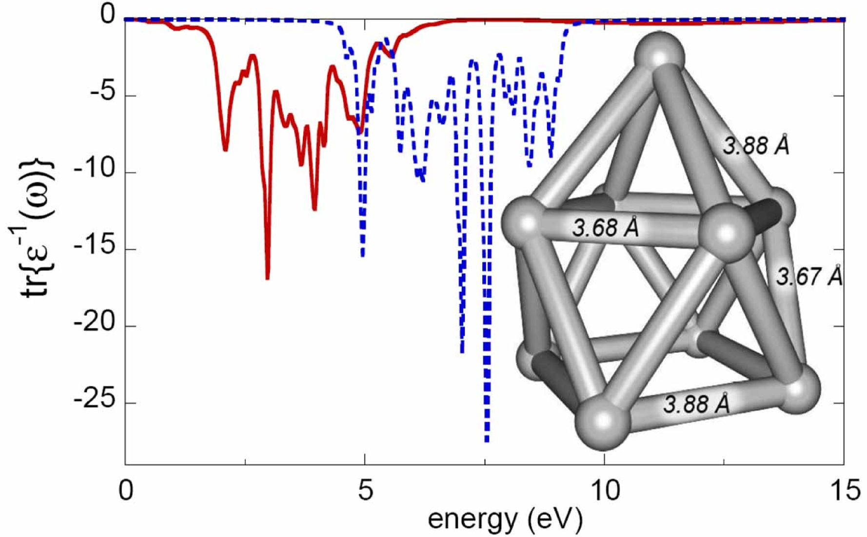
Figure 1: Trace over the inverse dielectric function in the GW-RPA (dashed line), and consistent GW (solid line) approaches for Na${}_{9}^{+}$. The inset shows the geometric structure used.

Before considering the QP properties of electrons, we examine the properties of the screened potential $W^{\mathrm{r}}(\omega)$. Figure 1 shows the trace over the imaginary part of the inverse dielectric function

$$\sum_{\alpha}{\mathrm{Im}}\,\varepsilon^{-1}_{\alpha\alpha}=\sum_{\alpha}(v\cdot{\mathrm{Im}}\chi^{\mathrm{r}})_{\alpha\alpha}.$$ (56)

In the GW-RPA method, the finite width of the peaks for $\varepsilon^{-1}$ is due to a phenomenological damping of $\Gamma=0.1~{}\mathrm{eV}$ instead of the scattering term in Eq. (49). Several peaks arising from resonances in the discrete level system are visible in the spectrum. We compare the RPA result with the consistent GW case, calculated using in Eq. (51) for $\Delta$ a quasiparticle broadening of $\gamma=0.25$ eV for the HF energies. One observes a drastic red shift of the whole spectrum by about 3 eV, together with a redistribution of spectral weight and a decrease of the “bandwidth” of the imaginary part of the inverse dielectric function, a typical correlation effect. This trend is in agreement with Ref ShirleyMartin , where a sizable change of QP energies in atomic systems was obtained when going from the GW-RPA to a GW calculation including exchange effects in the density-density correlation function.

Figure 2: Upper panel: Imaginary part of the self-energy for the HOMO (solid black line) and the LUMO (dashed grey line) of Na${}_{9}^{+}$, calculated in consistent GW approximation. Lower panel: The real part of the self-energy for the HOMO in GW-RPA (dashed blue line) and consistent GW (solid red line).

That this change is an improvement of the dynamically screened potential in the consistent GW calculation over the GW-RPA result is substantiated by evaluating the f-sum rule for finite systems. This relation is a measure of the quality of an approximation for $\varepsilon^{-1}$ and is directly related to the particle number conservation law at the two-particle level. A derivation of the f-sum rule for finite systems is presented in Appendix A. We find that for the consistent GW calculation, the $f$-sum rule Eq. (75) is fulfilled to better than $0.05\%$, whereas the GW-RPA violates it by 280%. This is a clear indication of the well-known fact that the RPA approximation is consistent only with Hartree Green’s functions Baym-Kadanoff:PR ; TammeSchepe and inconsistent for other approximate single-particle Green’s functions Szymansky . This restriction and inconsistency is removed at the consistent GW level.

Next, we use $W^{\mathrm{r}}$ on the level of GW-RPA and consistent GW, respectively, as input to the GW calculation of the QP properties. As a numerical check for the computational procedure, the normalization of the spectral function, i.e., particle number conservation on the single-particle level, is fulfilled to better than 0.1%.

Figure 3: Spectral function of the single-particle state with lowest energy for Na₄, Na${}_{9}^{+}$ and Na${}_{21}^{+}$ for HF (dotted black line), GW-RPA (dashed blue line) and consistent GW (solid red line) calculated with $\hbar\gamma_{\mathrm{bg}}=0.05$ eV. The insets show the geometric structure used for Na₄, and the dependence of the QP broadening on the background damping for Na${}_{9}^{+}$ and Na${}_{21}^{+}$.

Concerning the QP properties, we first discuss properties of the HOMO and LUMO in Na${}_{9}^{+}$. The upper panel of Fig. 2 depicts the energy dependence of $\mathrm{Im}\Sigma^{\mathrm{r}}$ in the consistent GW approximation. Inside the gap, it drops nearly to zero, leading to long lifetimes for states around the HOMO-LUMO gap (in agreement with the results from Ref YaroslavHubner ). The renormalized single-particle energies are obtained by solving the Dyson equation Eq. (9) where we add a constant background damping $i\hbar\gamma_{\mathrm{bg}}$ to $\Sigma^{\mathrm{corr}}(\omega)$ to avoid numerical problems due to the small damping near the HOMO-LUMO gap. The lower panel of Fig. 2 shows the real part of the retarded self-energy $\Sigma^{\mathrm{corr}}$. To determine the QP energies, we note that QP poles in the retarded Green’s function in Eq. (9) result if the real part of the denominator vanishes, i.e., if

$$\hbar\omega-\epsilon_{n}^{\mathrm{HF}}=\Sigma^{\mathrm{corr}}_{nn}(\omega).$$ (57)

The solution of Eq. (57) corresponds to finding the intersection of the function $\mathrm{Re}\Sigma^{\mathrm{corr}}(\omega)$ with the straight line $\hbar\omega-\epsilon^{\mathrm{HF}}_{n}$. This line is also shown in Fig. 2.

The QP broadening is then the value of $\mathrm{Im}\Sigma^{\mathrm{corr}}$ at the QP energy. The GW-RPA and consistent GW lead to different predictions for the size of the energy difference between the HOMO and the LUMO. In Table 1 we compare the calculated values of the gap with other theories and also experiment for the cases when data is available in the literature. Notice that in the case of Na₄ our method yields a HOMO-LUMO gap of 3.4 eV which is in very good agreement with the experimental value of 3.35 eV from photoelectron spectroscopy exp1 ; exp2 .

Table 1: The values of the energy gaps (in eV) between the HOMO and the LUMO for the studied Na clusters.

	Na4	Na${}_{9}^{+}$	Na${}_{21}^{+}$
HF	3.60	4.49	2.71
GW-RPA	3.56	4.31	2.59
consistent GW	3.40	4.14	2.44
literature	3.00 a	3.38 b
	3.35$\pm$0.2 c
a DFT+GW-RPA, from Ref. onida-prl .
b self-consistent GW-RPA, from Ref. YaroslavHubner .
c experiment, from Ref. exp1 ; exp2 .

From the spectral function, one can read off level shifts, broadening and redistribution of spectral weight. These features, important for states away from the HOMO and the LUMO, are experimentally accessible. Figure 3 shows the spectral functions of the single-particle state with the lowest energy for Na₄, Na${}_{9}^{+}$ and Na${}_{21}^{+}$, i.e., HOMO$-1$, HOMO$-3$ and HOMO$-9$, respectively. The insets show the dependence of the width (FWHM) of the QP peak on $\gamma_{\rm bg}$ used in the self-consistent GW calculation. Extrapolating to zero, one obtains the QP widths due to Coulomb correlations: for Na${}_{9}^{+}$, the QP broadening is 0.085 (0.02) eV for the consistent GW (GW-RPA). For Na${}_{21}^{+}$, the QP broadening is 0.29 (0.11) eV for the consistent GW (GW-RPA). For Na₄, this intrinsic QP width is on the order of the background broadening $\hbar\gamma_{\mathrm{bg}}=0.03$ eV and an extrapolation would be less accurate. While GW-RPA shows only a weak broadening of the QP peak, the consistent GW, as expected, yields a much broader main QP peak, together with a more pronounced redistribution of spectral weight that reaches lower energies with increasing cluster size. In terms of lifetimes, the QP broadenings of the lowest energy states give 7.74 fs for Na${}_{9}^{+}$ and 2.26 fs for Na${}_{21}^{+}$, in the case of the consistent GW approach. The order of magnitude of the lifetime values is in agreement with experiment, where the lifetime of the plasmon resonance in Na${}_{93}^{+}$ was found to be 10 fs; expLifetime1 also, in second harmonic generation time-resolved measurements on larger surface-supported Na clusters the same lifetime was obtained for a cluster size of about 25 nm SGHlifetime .

IV Conclusions

In conclusion, we have studied the effect of Coulomb correlations on the QP properties of electrons in metallic clusters within the framework of GW theory. Employing a linear-response calculation of the density-density correlation function allows us to obtain a conserving dynamically screened potential including finite, non-phenomenological damping. We analyze two approximations for the kinetic equation for the density response. One corresponds to the standard GW-RPA for the dielectric function based on HF energies and wave functions. The other one includes mean-field direct and exchange as well as correlation contributions to the dielectric function and the self-energy. The latter approximation is based on a consistent treatment of one- and two-particle correlations within the GW approximation. It is conserving in the sense of Baym and Kadanoff on the one and two-particle levels, and therefore fulfills the $f$-sum rule. Compared to GW-RPA, we find differences in the spectral function peak positions of up to 1 eV and differences in the QP broadening of more than a factor of 3 due to modifications of the screened Coulomb potential.

G.P and W.H. would like to acknowledge the support from the Schwerpunktprogramm SPP 1153 of the German Research Foundation.

Appendix A The $f$-sum rule for finite systems

In this Appendix we show how the $f$-sum rule for the density-density correlation function or, equivalently, for the inverse dielectric function for finite systems follows from particle-number conservation. To this end, we define the quantity

$$C(\vec{r}_{1},\vec{r}_{2};t_{1})\equiv i\hbar\frac{\partial}{\partial t_{1}}\left<[\rho(1),\rho(2)]\right>_{t_{1}=t_{2}},$$ (58)

where the angular brackets indicate an equilibrium averaging, and $\rho(1)=\psi^{{\dagger}}(1)\psi(1)$ is the particle density operator expressed by the field creation and destruction operators. We then evaluate Eq. (58) using the particle-number conservation condition, and finally relate $C$ to the Fourier transform of the density-correlation function.

To evaluate Eq. (58), we employ the continuity equation

$$\frac{\partial\rho(1)}{\partial t_{1}}+\nabla_{1}\cdot\vec{\jmath}(1)=0,$$ (59)

which is a statement of particle-density conservation in operator form. Here, the current density operator is given by

$$\vec{\jmath}(1)=\left.\frac{\hbar}{2im}\left(\nabla_{1}-\nabla_{1^{\prime}}\right)\psi^{{\dagger}}(1^{\prime})\psi(1)\right|_{1^{\prime}=1^{+}}.$$ (60)

Using (59) and (60), Eq. (58) yields

$$\qquad C(\vec{r}_{1},\vec{r}_{2};t_{1})=\\ \frac{\hbar^{2}}{2m}\left<\big{[}\nabla_{1}^{2}\psi^{{\dagger}}(1)\psi(1)-\psi^{{\dagger}}(1)\nabla_{1}^{2}\psi(1),\rho(2)\big{]}\right>_{t_{1}=t_{2}}.$$ (61)

Computing the commutator in a straightforward manner, one obtains

$$C(\vec{r}_{1},\vec{r}_{2};t_{1})= \frac{\hbar^{2}}{2m}\big{[}\left<\nabla^{2}_{1}\psi^{{\dagger}}(1)\psi(2)+\psi^{{\dagger}}(2)\nabla^{2}_{1}\psi(1)\right>_{t_{1}=t_{2}}\delta(\vec{r}_{1}-\vec{r}_{2})$$ (62)

$$\quad-\left<\psi^{{\dagger}}(1)\psi(2)+\psi^{{\dagger}}(2)\psi(1)\right>_{t_{1}=t_{2}}\nabla^{2}_{1}\delta(\vec{r}_{1}-\vec{r}_{2})\big{]}.$$

This expression cannot be treated further without integrating over $\vec{r}_{1}$ and $\vec{r}_{2}$ with smooth but otherwise arbitrary test functions. Choosing the test functions to be plane waves $e^{-i\vec{q}\cdot\vec{r}_{1}}$ and $e^{i\vec{q}\cdot\vec{r}_{2}}$, we evaluate the quantity

$$C_{\vec{q}\vec{q}}(t_{1})=\int e^{-i\vec{q}\cdot\vec{r}_{1}}C(\vec{r}_{1},\vec{r}_{2};t_{1})e^{i\vec{q}\cdot\vec{r}_{2}}{\mathrm{d}}^{3}r_{1}{\mathrm{d}}^{3}r_{2}.$$ (63)

From Eq. (62), one has

$$C_{\vec{q}\vec{q}}(t_{1})=\mbox{} \frac{\hbar^{2}}{2m}\int\left<\nabla^{2}_{1}\psi^{{\dagger}}(1)\psi(1)+\psi^{{\dagger}}(1)\nabla^{2}_{1}\psi(1)\right>{\mathrm{d}}^{3}r_{1}$$

$$\mbox{}-\frac{\hbar^{2}}{2m}\int\nabla^{2}_{1}\big{[}e^{-i\vec{q}\cdot\vec{r}_{1}}\left<\psi^{{\dagger}}(1)\psi(2)+\psi^{{\dagger}}(2)\psi(1)\right>_{t_{1}=t_{2}}\big{]}\delta(\vec{r}_{1}-\vec{r}_{2})e^{i\vec{q}\cdot\vec{r}_{2}}{\mathrm{d}}^{3}r_{1}{\mathrm{d}}^{3}r_{2},$$ (64)

which yields

$$C_{\vec{q}\vec{q}}(t_{1})=-\frac{\hbar^{2}}{m}\int\big{[}q^{2}\left<\rho(1)\right>-i\vec{q}\cdot\nabla_{1}\left<\rho(1)\right>\big{]}{\mathrm{d}}^{3}r_{1}.$$ (65)

This integral effectively extends over a finite volume because the integrand $\rho$ is the charge density of a finite system. The second contribution to the integral vanishes because it can be transformed into an integral over a closed surface lying outside of the charge density. The first integral is straightforward and yields

$$C_{\vec{q}\vec{q}}(t_{1})=\frac{\hbar^{2}q^{2}}{m}N_{\mathrm{e}},$$ (66)

where $N_{\mathrm{e}}$ is the total number of electrons in the system.

We now need to relate the commutator $C$ to the density-density correlation function, which is defined as

$$i\hbar\chi^{\mathrm{r}}(1,2)=\Theta(t_{1}-t_{2})\langle\left[\rho(1),\rho(2)\right]\rangle.$$ (67)

In equilibrium, the correlation function depends only on the difference of the times $t_{1}$ and $t_{2}$ Kadanoff-Baym:Book . Using this property, one performs a Fourier transformation in $t_{1}-t_{2}$ and obtains for the imaginary part of $\chi^{\mathrm{r}}(\omega)$

$${\mathrm{Im}}\chi^{\mathrm{r}}(\vec{r}_{1},\vec{r}_{2};\omega)=-\frac{1}{2\hbar}\langle\left[\rho(\vec{r}_{1},\omega),\rho(\vec{r}_{2})\right]\rangle.$$ (68)

On the other hand, Fourier transformation of Eq. (58) yields

$$C(\vec{r}_{1},\vec{r}_{2};t_{1})=i\hbar\int_{-\infty}^{+\infty}\frac{\mathrm{d}\omega}{2\pi}\omega\,\langle\left[\rho(\vec{r}_{1},\omega),\rho(\vec{r}_{2})\right]\rangle,$$ (69)

so that we obtain

$$C(\vec{r}_{1},\vec{r}_{2};t_{1})=-\frac{\hbar^{2}}{\pi}\int_{-\infty}^{+\infty}{\mathrm{d}}\omega\,\omega{\mathrm{Im}}\chi^{\mathrm{r}}(\vec{r}_{1},\vec{r}_{2};\omega).$$ (70)

Inserting this result for $C$ in (63) and equating it with (66), one obtains

$$\frac{q^{2}}{m}N_{\mathrm{e}}=-\frac{1}{\pi}\int_{-\infty}^{+\infty}{\mathrm{d}}\omega\omega\int{\rm e}^{-i\vec{q}\cdot\vec{r}_{1}}{\rm Im}\chi^{\rm r}(\vec{r}_{1},\vec{r}_{2};\omega){\rm e}^{i\vec{q}\cdot\vec{r}_{2}}{\mathrm{d}}^{3}r_{1}{\mathrm{d}}^{3}r_{2}.$$ (71)

The $f$-sum rule for finite systems can now be derived by expanding $\chi^{\mathrm{r}}$ on the RHS of Eq. (71) into the basis functions (HF orbitals) $\{\varphi_{n}(\vec{r})\}$. Thus

$$-\frac{2}{\pi}\int_{0}^{\infty}d\omega\,\omega\sum_{n_{1}\dots n_{4}}P_{n_{1}n_{3}}(-\vec{q})P_{n_{2}n_{4}}(\vec{q})\mathrm{Im}\left<n_{1}n_{2}\left|\chi^{\rm r}(\omega)\right|n_{3}n_{4}\right>=\frac{q^{2}}{m}N_{\rm e},$$ (72)

where we have defined the overlaps

$$P_{n_{1}n_{2}}(\vec{q})=\int{\rm e}^{i\vec{q}\cdot\vec{r}}\varphi^{*}_{n_{1}}(\vec{r})\varphi_{n_{2}}(\vec{r}){\mathrm{d}}^{3}r$$ (73)

and used the symmetry of $\chi^{\mathrm{r}}(-\omega)=\chi^{\mathrm{r}}(\omega)^{*}$. Expanding the exponential function yields

$$P_{n_{1}n_{2}}(\vec{q})=\int\varphi^{*}_{n_{1}}(\vec{r})\left(i\vec{q}\cdot\vec{r}\right)\varphi_{n_{2}}(\vec{r})\,{\mathrm{d}}^{3}r+\text{terms of higher order in }q.$$ (74)

Note that there is no $q$-independent term because the basis functions $\{\varphi_{n}(\vec{r})\}$ are orthogonal for $n_{1}\neq n_{2}$. Using Eq. (74) in Eq. (72), dividing by $q^{2}$ and then letting $q\rightarrow 0$ yields the $f$-sum rule for finite systems:

$$\int_{0}^{\infty}{\rm d}\omega\,\omega\sum_{n_{1}\dots n_{4}}\left(\vec{n}\cdot\vec{r}_{n_{1}n_{3}}\right)\left(\vec{n}\cdot\vec{r}_{n_{2}n_{4}}\right)\left[-\mathrm{Im}\langle n_{1}n_{2}|\chi^{\rm r}(\omega)|n_{3}n_{4}\rangle\right]=\frac{\pi}{2m}N_{e}.$$ (75)

Here $\vec{n}$ is a unit vector in an arbitrary direction and we have defined the matrix element of the position operator

$$\vec{r}_{n_{1}n_{2}}=\int\varphi^{*}_{n_{1}}(\vec{r})\,\vec{r}\,\varphi_{n_{2}}(\vec{r})\,{\mathrm{d}}^{3}r.$$ (76)

Appendix B Comparison with Bethe-Salpeter Equation

In this Appendix, we wish point out the differences and similarities of our calculation to the BS equation approach, which has been employed for the calculation of absorption spectra in a variety of systems, including finite systems such as Na₄ onida-prl .

The following derivations follow closely the arguments of Ref. Baym-Kadanoff:PR , which uses equilibrium one- and two-particle Green’s functions for complex times. Consequently, the time integrations extend over $0<it<1/(k_{\mathrm{B}}T)$, where $k_{\mathrm{B}}$ is Boltzmann’s constant and $T$ is the temperature Kadanoff-Baym:Book . To extract the real-time Green’s functions from this formalism one needs to perform an analytical continuation to real times. An equivalent procedure, which is closer to the formal development in this paper, is to keep the notation of Ref. Baym-Kadanoff:PR , but to interpret the Green’s functions as real-time Green’s functions defined on the Keldysh contour, and the integrals over time as Keldysh contour integrals.

We work with correlation functions that are dependent on space-time variables instead of the the quantities labeled by HF spin orbitals introduced in Eqs. (7) and (8). We begin by defining the four-point correlation function

$$i\hbar L(12,34)=\langle T[\psi(1)\psi(3)\psi^{{\dagger}}(2)\psi^{{\dagger}}(4)]\rangle-\langle T[\psi(1)\psi^{{\dagger}}(2)]\rangle\langle T[\psi(3)\psi^{{\dagger}}(4)]\rangle,$$ (77)

where $T$ ensures the time-ordering on the Keldysh contour. Introducing an external disturbance $U(3,4)$ one can generate the four-point function by the functional derivative

$$L(12,34)=-i\hbar\left.\frac{\delta G(1,2)}{\delta U(3,4)}\right|_{U=0}.$$ (78)

The density-density correlation function used earlier in this paper is given in terms of the four-point correlation function by

$$\chi(1,2)=L(11^{+},22^{+})$$ (79)

where $1^{+}=(\vec{r}_{1}\sigma_{1}t_{1}^{+})$ and $t_{1}^{+}$ is a time on the Keldysh contour infinitesimally larger than $t_{1}$. The screened potential $W$ is then determined by

$$W(1,2)=v(1,2)+V(1,\bar{3})\chi(\bar{3},\bar{4})V(\bar{4},2).$$ (80)

Here and in the following the convention is used that repeated space, spin, and time indices with an overbar are integrated over space and time and summed over spin indices. Further, the abbreviation

$$V(1,2)=\delta(t_{1}-t_{2})\delta_{\sigma_{1},\sigma_{2}}v(\vec{r}_{1}-\vec{r}_{2})$$ (81)

has been introduced. For the case of the independent-particle approximation, this correlation function is given by

$$L^{0}(12,34)=-i\hbar G(1,3)G(4,2).$$ (82)

To arrive at an equation for $L$, one starts with the Dyson equation for the Green’s function:

$$G^{-1}(1,2)=G^{-1}_{0}(1,2)-U(1,2)-\Sigma(1,2).$$ (83)

In the GW approximation, the self-energy consists of the unscreened direct (Hartree) term and the screened exchange (GW) term:

$$\Sigma(1,2)=-i\hbar\delta(1-2)V(1,\bar{3})G(\bar{3},\bar{3}^{+})+i\hbar G(1,2)W(2,1)$$ (84)

From the identity $G(1,\bar{3})G^{-1}(\bar{3},2)=\delta(1-2)$, it follows

$$\frac{\delta G(1,2)}{\delta U(3,4)}=-G(1,\bar{5})\frac{\delta G^{-1}(\bar{5},\bar{6})}{\delta U(3,4)}G(\bar{6},2).$$ (85)

After calculating the functional derivative of the inverse Green’s function with respect to $U$ from Eq. (83), one obtains

$$\frac{\delta G(1,2)}{\delta U(3,4)}=\mbox{}G(1,\bar{5})G(\bar{6},2)\Big{[}\delta(3-\bar{5})\delta(4-\bar{6})+\frac{\delta\Sigma(\bar{5},\bar{6})}{\delta U(3,4)}\Big{]}.$$ (86)

Inserting in Eq. (86) the self-energy from (84), one obtains after performing the derivative with respect to $U$ (neglecting terms with $\delta W/\delta U$) and using the definition (78), an equation for the four-point correlation function function that is consistent with the GW self-energy

$$L(12,34)=L^{0}(12,34)+L^{0}(12,\bar{5}\bar{6})[K_{\mathrm{HF}}(\bar{5}\bar{6},\bar{7}\bar{8})+K_{\mathrm{c}}(\bar{5}\bar{6},\bar{7}\bar{8})]L(\bar{7}\bar{8},34)$$ (87)

In Eq. (87), the contributions to the kernel consist of the bare Hartree-Fock contribution

$$K_{\mathrm{HF}}(12,34)=\delta(1-2)\delta(3-4)V(1,3)-\delta(1-3)\delta(2-4)V(1,2),$$ (88)

and the correlation term

$$K_{\mathrm{c}}(12,34)=-\delta(1-3)\delta(2-4)V(1,\bar{5})\chi(\bar{5},\bar{6})V(\bar{6},2).$$ (89)

It is apparent that the screened Coulomb interaction enters only in the correlation contribution, which can be evaluated after the density-density correlation function is specified. A natural starting point is the noninteracting density-density correlation function

$$\chi^{0}(1,2)=-i\hbar G(1,2)G(2,1),$$ (90)

according to Eq. (82). Then the correlation contribution takes the form

$$K_{\mathrm{c}}(12,34)=-\delta(1-3)\delta(2-4)V(1,\bar{5})L^{0}(\bar{5}\bar{5},\bar{6}\bar{6})V(2,\bar{6})$$ (91)

The diagrammatic representation of Eq. (87) with kernels (88) and (91) is shown in Fig. 4. The correlation contribution in this approximation is due to particle-hole pair excitation processes Baym-Kadanoff:PR ; Kwong-Bonitz .

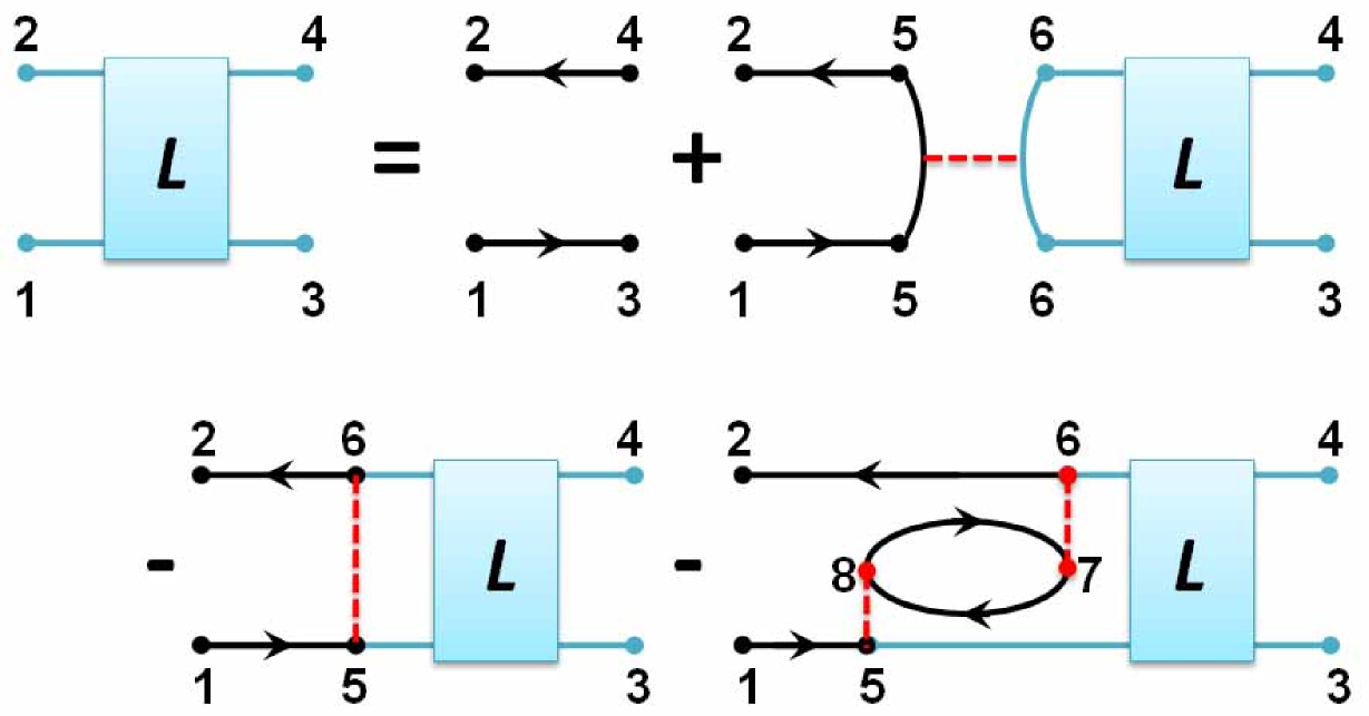
Figure 4: Diagrammatic representation of the BS equation (87). The square represents the four-point correlation function defined in Eq. (78), the two electron-hole lines stand for the independent particle correlation function, and the dashed lines are for the bare Coulomb potential.

To make the connection with the BS equation with screened-exchange kernel, one can combine the $K_{\mathrm{HF}}$ and $K_{\mathrm{c}}$ contributions to obtain

$$L(12,34)=L^{0}(12,34)+L^{0}(12,\bar{5}\bar{6})K_{\mathrm{SX}}(\bar{5}\bar{6},\bar{7}\bar{8})L(\bar{7}\bar{8},34)$$ (92)

where

$$K_{\mathrm{SX}}(12,34)=\mbox{} \delta(1-2)\delta(3-4)V(1,3)-W(12,34)$$ (93)

$$W(12,34)=\mbox{} \delta(1-3)\delta(2-4)[V(1,2)+V(1,\bar{5})L^{0}(\bar{5}\bar{5},\bar{6}\bar{6})V(\bar{6},2)].$$ (94)

This way, a general BS equation with screened-exchange kernel and dielectric function

$$\varepsilon^{-1}(1,2)=\delta(1-2)+V(1,\bar{3})\chi^{0}(\bar{3},2)$$ (95)

is recovered. However, there is an important difference between the approach presented here and GW-based BS equation calculations: Usually the BS equation is employed to determine the absorption using the screened potential as an ingredient. We compute the density-density correlation function $\chi$, which is related to $L$ via Eq. (79), in order to determine the screened potential $W$. Thus the meaningful comparison should be made between RPA-like inverse dieletric functions, and the $\varepsilon^{-1}$ resulting from the density-density correlation function, or Eq. (87). As already mentioned in connection with Eq. (54), retaining only the Hartree term in Eq. (87) is already equivalent to the RPA Baym-Kadanoff:PR ; Kwong-Bonitz , so that the inclusion of exchange and scattering/dephasing contributions represents a considerable improvement over the RPA. In addition, this improvement is reached in a consistent manner, i.e., we can be reasonably sure that we have not sacrificed accuracy at a different level in the calculation.

Finally, we would like to relate Eq. (87) together with (79) to our derivation of the central Eq. (49) for $\chi^{\mathrm{r}}$ using nonequilibrium Green’s functions techniques. To facilitate the comparison, we perform a partial resummation of Eq. (87). To display the HF contribution at the two-particle level we define

$$L_{\mathrm{HF}}(12,34)=L^{0}(12,34)+L^{0}(12,\bar{5}\bar{6})K_{\mathrm{HF}}(\bar{5}\bar{6},\bar{7}\bar{8})L_{\mathrm{HF}}(\bar{7}\bar{8},34).$$ (96)

This allows one to rewrite Eq. (87) in the form

$$L(12,34)=L_{\mathrm{HF}}(12,34)+L_{\mathrm{HF}}(12,\bar{5}\bar{6})K_{\mathrm{c}}(\bar{5}\bar{6},\bar{7}\bar{8})L(\bar{7}\bar{8},34),$$ (97)

If one demands consistency also at the HF level then it is important that the HF Eq. (97) for the four-point functions use $L^{0}$ defined in Eq. (82) constructed from HF single-particle Green’s functions.

Equation (97) is still defined for time arguments on the Keldysh contour, but it shows a formal similarity to Eq. (49) in that it consistently displays the HF contributions on the one-particle and two-particle levels, and separates out the correlation contributions, as it is also evident in Eq. (49). To make use of Eq. (97), one has to compute all the different Keldysh components of these four-point quantities 4index . Only after the full four-point correlation function $L$ is calculated, one could obtain via Eq. (79) the retarded density-density correlation function needed to determine the screened Coulomb potential for the GW calculation. Our derivation using kinetic equations and the generalized Kadanoff-Baym ansatz, on the other hand, is a way to derive a closed set of equations that depends only on two-time quantities and obeys the consistency condition derived from density/current conservation. The generalized Kadanoff-Baym ansatz makes the calculational procedure in principle self-consistent because it connects the kinetic Green’s functions in the correlation contributions with the retarded (equilibrium) Green’s functions. It also ensures that the calculation deals exclusively with two-time quantities, which in equilibrium depend only on the time difference, so that after Fourier transformation both the one-particle and two-particle correlation functions used in the calculation can be given a quasiparticle interpretation.

References

- (1) L. Hedin, Phys. Rev. 139, A796 (1965).
- (2) G. Onida, L. Reining, and A. Rubio, Rev. Mod. Phys. 74, 601 (2002).
- (3) F. Aryasetiawan and O. Gunnarsson, Rep. Prog. Phys. 61, 237 (1998).
- (4) V. P. Zhukov, F. Aryasetiawan, E. V. Chulkov, and P. M. Echenique, Phys. Rev. B 65, 115116 (2002).
- (5) M. Rohlfing, N.-P. Wang, P. Kruger, and J. Pollmann, Phys. Rev. Lett. 91, 256802 (2003).
- (6) B. Holm and U. von Barth, Phys. Rev. B 57, 2108 (1998).
- (7) W. D. Schöne and A. G. Eguiluz, Phys. Rev. Lett. 81, 1662 (1998).
- (8) S. V. Faleev, M. van Schilfgaarde, and T. Kotani, Phys. Rev. Lett 93, 126406 (2004).
- (9) P. Sun and G. Kotliar, Phys. Rev. Lett 92, 196402 (2004).
- (10) W. Ku and A. G. Eguiluz, Phys. Rev. Lett 89, 126401 (2002).
- (11) G. D. Mahan and B. E. Sernelius, Phys. Rev. Lett. 62, 2718 (1989).
- (12) A. Schindlmayr and R. W. Godby, Phys. Rev. Lett. 80, 1702 (1998).
- (13) D. Tamme, R. Schepe, and K. Henneberger, Phys. Rev. Lett. 83, 241 (1999).
- (14) Y. Takada, Phys. Rev. Lett. 87, 226402 (2001).
- (15) S. Grabowski, M. E. Garcia, and K. H. Bennemann, Phys. Rev. Lett. 72, 3969 (1994).
- (16) M. Quijada, R. D. Muiño, and P. M. Echenique, Nanotechnology 16, S176 (2005).
- (17) Y.Pavlyukh and W. Hübner, Phys. Lett. A 327, 241 (2004).
- (18) G. Baym and L. P. Kadanoff, Phys. Rev. 124, 287 (1961).
- (19) F. Green, D. Neilson, and J. Szymanski, Phys. Rev. B 31, 2779 (1985).
- (20) G. Strinati, H. J. Mattausch, and W. Hanke, Phys. Rev. B 25, 2867 (1982).
- (21) N.-H. Kwong and M. Bonitz, Phys. Rev. Lett. 84, 1768 (2000).
- (22) G. Baym, Phys. Rev. 127, 1391 (1962).
- (23) L. Hedin and S. Lundqvist, Solid State Physics 23, 1 (1969).
- (24) C. O. Almbladh, J. Phys. 35, 127 (2006).
- (25) R. D. Sole, L. Reining, and R. W. Godby, Phys. Rev. B 49, 8024 (1994).
- (26) E. L. Shirley and R. M. Martin, Phys. Rev. B 47, 15404 (1993).
- (27) L. P. Kadanoff and G. Baym, Quantum Statistical Mechanics (Addison-Wesley, New York, 1989).
- (28) A. V.Kuznetsov, Phys. Rev. B 44, 8721 (1991).
- (29) W. D. Kraeft, M. Schlanges, J. Vorberger, and H. E. DeWitt, Phys. Rev. E 66, 46405 (2002).
- (30) R. Binder and S. W. Koch, Prog. Quant. Electr. 19, 307 (1995).
- (31) D. Kremp, M. Schlanges, and W. D. Kraeft, Quantum Statistics of Nonideal Plasmas (Springer, Berlin Heidelberg New York, 2005).
- (32) N. E. Dahlen and R. van Leeuwen, Phys. Rev. Lett. 98, 153004 (2007).
- (33) F. Jahnke, M. Kira, and S. W. Koch, Z. Phys. B: Condens. Matter 104, 559 (1997).
- (34) S. Ismail-Beigi and S. G. Louie, Phys. Rev. Lett. 90, 076401 (2003).
- (35) W. R. Wadt and P. J. Hay, J. Chem. Phys 82, 284 (1985).
- (36) K. I. Peterson, P. D. Dao, R. W. Farley, and A. W. Castleman, Jr., J. Chem. Phys. 80, 1780 (1984).
- (37) K. M. McHugh, J. G. Eaton, G. H. Lee, H. W. Sarkas, L. H. Kidder, J. T. Snodgrass, M. R. Manaa, and K. H. Bowen, J. Chem. Phys. 91, 3792 (1989).
- (38) G. Onida, L. Reining, R. W. Godby, R. D. Sole, and W. Andreoni, Phys. Rev. Lett. 75, 818 (1995).
- (39) R. Schlipper, R. Kusche, B. von Issendorff, and H. Haberland, Phys. Rev. Lett. 80, 1194 (1998).
- (40) J.-H. Klein-Wiele, P. Simon, and H.-G. Rubahn, Phys. Rev. Lett. 80, 45 (1998).
- (41) Note that it is hard to give correlation functions depending on four Keldysh indices a direct physical meaning, as it is possible for, say, the retarded and kinetic components of Green’s functions with two Keldysh indices; see, e.g., Ref. Kremp:Book .