Exceptional points in the spectra of atoms in external fields

Abstract

We investigate exceptional points, which are branch point singularities of two resonance eigenstates, in spectra of the hydrogen atom in crossed external electric and magnetic fields. A procedure to systematically search for exceptional points is presented, and their existence is proven. The properties of the branch point singularities are discussed with effective low-dimensional matrix models, their relation with avoided level crossings is analyzed, and their influence on dipole matrix elements and the photoionization cross section is investigated. Furthermore, the rare case of a connection between three resonances almost forming a triple-degeneracy in the form of a cubic root branch point is discussed.

I Introduction

A special type of degeneracy in parameter-dependent resonance spectra, namely “exceptional points” Kato (1966); Heiss (1999), has recently attracted growing attention theoretically Heiss (2000); Heiss and Sannino (1990); Berry and O’Dell (1998); Cejnar et al. (2007); Klaiman and Cederbaum (2008); Lee et al. (2008); Müller and Rotter (2008) as well as experimentally Philipp et al. (2000); Dembowski et al. (2001, 2003, 2004); Dietz et al. (2007); Stehmann et al. (2004). Exceptional points can be found in systems which depend on at least two real valued parameters. They are positions in the parameter space at which usually two energy eigenvalues pass through a branch point singularity, i.e., the two eigenvalues can mathematically be described by two branches of the same analytic function and the exceptional point represents the branch point singularity. In this case, also the eigenvectors, or wave functions, pass through a branch point singularity and, hence, are identical. The occurrence of a geometric phase Berry (1984) is one of the important consequences of exceptional points Heiss (1999).

Within the framework of the linear Schrödinger equation, the existence of resonances, i.e., decaying unbound states is important for the appearance of exceptional points because the coalescence of two discrete eigenstates with identical eigenvectors is not possible in the spectra of Hermitian Hamiltonians with potentials, which describe bound states. Here, always a set of orthogonal eigenstates, which never can become identical, exists. For resonances, the situation is different. Their eigenstates can become identical. One possibility of obtaining the resonances is the complex rotation method Reinhardt (1982); Ho (1983); Moiseyev (1998), which leads to non-Hermitian Hamiltonians in the spectra of which resonances are uncovered as complex eigenvalues.

Physical systems in which exceptional points can appear have to depend on at least a two-dimensional parameter space. If exceptional points are to be observable it must be possible to adjust these parameters in a sufficiently wide range of the parameter space. Furthermore, the complex energy eigenvalues, typically the positions (frequencies or energies) and widths of resonances, must be accessible with a high precision. Examples are discussed, e.g., for complex atoms in laser fields Latinne et al. (1995), a double $\delta$ well Korsch and Mossmann (2003), the scattering of a beam of particles by a double barrier potential Hernández et al. (2006), non-Hermitian Bose-Hubbard models Graefe et al. (2008), or models used in nuclear physics von Brentano and Philipp (1999). The resonant behavior of atom waves in optical lattices Oberthaler et al. (1996) shows structures originating from exceptional points Berry and O’Dell (1998), and they can be found in nonlinear quantum systems. The stationary solutions of the Gross-Pitaevskii equation describing Bose-Einstein condensates exhibits a coalescence of two states due to the nonlinearity of the equation, which turns out to be a branch point singularity of the energy eigenvalues and wave functions Cartarius et al. (2008); Rapedius and Korsch (2009). However, the phenomenon of exceptional points in physics is not restricted to quantum mechanics. Acoustic modes in absorptive media Shuvalov and Scott (2000) represent a mechanical system, in which branch point singularities appear. Manifestations of exceptional points can also be seen in optical devices Pancharatnam (1955); Berry (1994); Wiersig et al. (2008); Klaiman et al. (2008). The most detailed experimental analysis of exceptional points has been carried out for the resonances of microwave cavities Philipp et al. (2000); Dembowski et al. (2003); Dietz et al. (2007), which open the possibility of studying the properties of the complex resonance frequencies and the wave functions. In particular, the geometric phase has been demonstrated experimentally Dembowski et al. (2001, 2004).

Atoms in static external electric and magnetic fields are fundamental physical systems. As real quantum systems they are accessible both to experimental and theoretical methods and have, e.g., very successfully been used for comparisons with semiclassical theories Freund et al. (2002); Rao et al. (2001); Bartsch et al. (2003a, b). They provide a rich variety of physical phenomena such as Ericson fluctuations, which were discovered both in numerical studies Main and Wunner (1992, 1994) and experiments Stania and Walther (2005). Recently, the existence of exceptional points was reported and a method to detect them in an experiment with atoms was proposed Cartarius et al. (2007). Atoms in external fields are well suited to study the signatures originating from exceptional points in quantum spectra. The electric and magnetic field strengths span the two-dimensional parameter space required to provide the branch points.

It is the purpose of this paper to show how exceptional points can be detected systematically in spectra of the hydrogen atom in external fields and to discuss their properties in detail. Numerically exact resonance energies and eigenstates are determined by the complex rotation method Reinhardt (1982); Ho (1983); Moiseyev (1998). The permutation behavior of the resonances for closed parameter space loops is used to unambiguously find and verify the branch point singularities. Examples for exceptional points found in the system are presented. The shapes of the loops of the complex eigenvalues representing the resonances are explained with a two-dimensional matrix model. It is shown that single dipole matrix elements of two states coalescing at an exceptional point diverge whereas this behavior does not carry over to the observable photoionization cross section.

Besides the typical case, where an exceptional point consists of two resonances forming a square root branch point, higher degeneracies are possible. In this paper the rare case of a structure with three resonances almost forming a triple-coalescence in the form of a cubic root branch point is presented. It is shown how exceptional points are related to avoided crossings of the energies or widths of the resonances.

The paper is organized as follows. Sec. II summarizes the most important characteristics of exceptional points and demonstrates them with the help of an illustrative example. The Hamiltonian of the crossed-fields hydrogen atom is introduced in Sec. III, and the method to obtain the resonance eigenstates is presented. A procedure to find exceptional points in spectra of atoms in external fields is presented and applied in Sec. IV, in which also examples of branch point singularities are given. A two-dimensional matrix model used to explain the paths of the eigenvalues for parameter space loops is introduced and applied in Sec. V. The influence of exceptional points on dipole matrix elements and the photoionization cross section is discussed in Sec. VI. Three resonances almost forming a triple-coalescence are presented in Sec. VII, and the connection between exceptional points and avoided level crossings is investigated in Sec. VIII. Conclusions are drawn in Sec. IX.

II Exceptional points

II.1 Important properties

The typical case of an exceptional point is a position in a two-dimensional parameter space at which two eigenvalues pass through a branch point singularity. This behavior has important consequences for the associated eigenvalues and eigenvectors.

If one encircles the exceptional point in the parameter space, a typical permutation behavior of the eigenvalues can be observed Kato (1966). The two eigenvalues which represent the two branches of one analytic function with the singularity are interchanged after one circle around the exceptional point, whereas all further eigenvalues do not undergo a permutation. Away from the exceptional points the branching eigenvalues are different and each of them belongs to a distinct eigenvector. Accordingly, these eigenvectors undergo the same permutation as the eigenvalues, and at the exceptional points they likewise pass through a branch point singularity Kato (1966), i.e., there is only one linearly independent eigenvector for the two degenerate eigenvalues. In a matrix representation, the eigenvalues and eigenvectors form a normal block Günther et al. (2007); Seyranian et al. (2005), which distinguishes them from ordinary degeneracies where two eigenvalues belonging to two different analytic functions have the same value. Alongside the permutation of the eigenvectors a geometric phase appears. In the most common physical situation of a square root branch point resulting from a complex symmetric matrix, the geometric phase becomes manifest in the change in sign of one of the two eigenvectors Heiss (1999) and can be written in the form

$$[\bm{x}_{1},\bm{x}_{2}]\overset{\text{circle}}{\to}[\bm{x}_{2},-\bm{x}_{1}]\;,$$

where $\bm{x}_{1}$ and $\bm{x}_{2}$ are the eigenvectors permuted during the loop around the exceptional point.

It should be mentioned that the occurrence of the phenomenon is not restricted to two dimensions. In higher-dimensional parameter spaces of complex matrices, an exceptional “point” is always an object of co-dimension 2 Seyranian et al. (2005). That is, in two dimensions an exceptional point indeed appears as a point, whereas in three dimensions it is a one-dimensional object, or line, and in a four-dimensional parameter space it has the form of a two-dimensional “exceptional surface.”

II.2 A simple example in a non-Hermitian linear map

One of the simplest examples in which an exceptional point occurs, and which helps to understand many effects related to it, is described by the two-dimensional matrix Kato (1966)

$$\bm{M}(\kappa)=\left(\begin{array}[]{rr}1&\kappa\\ \kappa&-1\end{array}\right)$$ (1)

with the complex parameter $\kappa$. The two eigenvalues of the matrix are given by

$$\lambda_{1}=\sqrt{1+\kappa^{2}}\;,\quad\lambda_{2}=-\sqrt{1+\kappa^{2}}$$ (2)

and are obviously two branches of the same analytic function in $\kappa$. There are two exceptional points in the system, which appear at the complex conjugate values $\kappa_{\pm}=\pm\mathrm{i}$ as can easily be seen. The eigenvectors which belong to the two eigenvalues are

$$\bm{x}_{1,2}(\kappa)=\left(\begin{array}[]{c}-\kappa\\ 1\mp\sqrt{1+\kappa^{2}}\end{array}\right)\;.$$ (3)

They also depend on the parameter $\kappa$ and pass through a branch point singularity at the exceptional points $\kappa_{\pm}=\pm\mathrm{i}$, where the only linearly independent eigenvector reads $\bm{x}(\pm\mathrm{i})=(\mp\mathrm{i},1)$.

The branch point singularity leads to a characteristic behavior of the corresponding eigenvalues under changes of the parameters. If one chooses a closed loop in the parameter space and calculates the eigenvalues for a set of parameters on this loop, the permutation of the eigenvalues can be seen by plotting their paths in the complex energy plane. The situation is illustrated in Fig. 1.

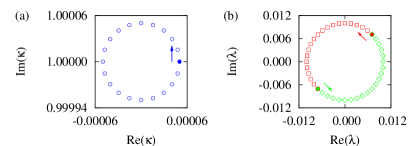
Figure 1: (Color online) (a) Circle in the parameter space $\kappa$ with the exceptional point $\kappa_{+}=\mathrm{i}$ as center point for the simple model (1). (b) Eigenvalues $\lambda_{1,2}$ calculated for the parameter values from (a) indicated by red squares and green diamonds, respectively. In this case each of the two eigenvalues traverses a semicircle. In (a) and (b) the filled symbols represent the first parameter value $\kappa_{0}$ and the corresponding eigenvalues $\lambda_{1,2}(\kappa_{0})$, respectively. The arrows point in the direction of progression.

Here, a circle $\kappa(\varphi)=\mathrm{i}+\varrho\mathrm{e}^{\mathrm{i}\varphi}$ around the singularity $\kappa_{+}=\mathrm{i}$ is traversed in the parameter space, which is shown in Fig. 1(a). After one revolution, the first eigenvalue marked by red squares has traveled to the starting point of the second marked by green diamonds, and vice versa. As a consequence, the path of each eigenvalue is not closed if one traversal of the loop in the parameter space is performed, but the path is closed if the parameter space loop is traversed twice. Of course, for the simple model it is also possible to demonstrate the half-circle structure analytically. If the parameter space curve described above is applied to the eigenvalues (2) one obtains, for $\varrho\ll 2$, the expansion

$$\lambda_{1,2} =\pm\sqrt{1+(\mathrm{i}+\varrho\mathrm{e}^{\mathrm{i}\varphi})^{2}}=\pm\sqrt{\varrho}\mathrm{e}^{\mathrm{i}\varphi/2}\sqrt{2\mathrm{i}+\varrho\mathrm{e}^{\mathrm{i}\varphi}}$$

$$\approx\pm\sqrt{2\varrho}\mathrm{e}^{\mathrm{i}\pi/4}\mathrm{e}^{\mathrm{i}\varphi/2}$$ (4)

or

$$\lambda_{1}=\sqrt{2\varrho}\mathrm{e}^{\mathrm{i}(\pi/4+\varphi/2)}\;,\quad\lambda_{2}=\sqrt{2\varrho}\mathrm{e}^{\mathrm{i}(5\pi/4+\varphi/2)}\;,$$ (5)

which reproduces the half-circles shown in Fig. 1 for a full parameter space loop $\varphi=0\dots 2\pi$ correctly.

III Hamiltonian and matrix representation

In this paper the hydrogen atom in static crossed electric and magnetic fields is investigated from the point of view of exceptional points. The electric field is assumed to point in the $x$-direction and the magnetic field is orientated along the $z$-axis. The Hamiltonian without relativistic corrections and finite nuclear mass effects Schmelcher and Cederbaum (1993) reads in atomic Hartree units

$$H=\frac{1}{2}\bm{p}^{2}-\frac{1}{r}+\frac{1}{2}\gamma L_{z}+\frac{1}{8}\gamma^{2}(x^{2}+y^{2})+fx\;,$$ (6)

where $\bm{p}$ is the kinetic momentum of the electron, $r$ its distance from the nucleus, and $L_{z}$ the $z$-component of the angular momentum. The Hamiltonian contains the Coulomb potential $\propto 1/r$, the paramagnetic term $\propto\gamma L_{z}$, the diamagnetic term $\propto\gamma^{2}(x^{2}+y^{2})$, and the potential due to the external electric field $\propto fx$.

For the numerical calculation of the energy eigenvalues in a matrix representation of the Hamiltonian (6) it is advantageous to transform the Schrödinger equation into dilated semiparabolic coordinates,

$$\mu=\frac{1}{b}\sqrt{r+z}\;,\quad\nu=\frac{1}{b}\sqrt{r-z}\;,\quad\varphi=\arctan\frac{y}{x}$$ (7)

with $r=\sqrt{x^{2}+y^{2}+z^{2}}$. For calculating the resonances of the system the complex rotation method Reinhardt (1982); Ho (1983); Moiseyev (1998) is used as a powerful tool Delande et al. (1991); Main and Wunner (1992, 1994). The complex scaling is included via the dilation parameter $b$, where the replacement

$$b^{2}=|b^{2}|\mathrm{e}^{\mathrm{i}\theta}$$ (8)

entails the complex rotation of the position vector

$$\bm{r}\to\mathrm{e}^{\mathrm{i}\theta}\bm{r}$$ (9)

and leads to the complex scaled and regularized Schrödinger equation

$$\bigg{\{}-2H_{0}+|b|^{4}\mathrm{e}^{\mathrm{i}2\theta}\gamma\left(\mu^{2}+\nu^{2}\right)\mathrm{i}\frac{\partial}{\partial\varphi}-\frac{1}{4}|b|^{8}\mathrm{e}^{\mathrm{i}4\theta}\gamma^{2}\\ \times\mu^{2}\nu^{2}\left(\mu^{2}+\nu^{2}\right)-2|b|^{6}\mathrm{e}^{\mathrm{i}3\theta}f\mu\nu\left(\mu^{2}+\nu^{2}\right)\cos\varphi\\ +4|b|^{2}\mathrm{e}^{\mathrm{i}\theta}+\left(\mu^{2}+\nu^{2}\right)\bigg{\}}\mathrm{e}^{-\mathrm{i}2\theta}\psi=2|b|^{4}E\left(\mu^{2}+\nu^{2}\right)\psi$$ (10a)

with the term

$$H_{0}=-\frac{1}{2}(\Delta_{\mu}+\Delta_{\nu})+\frac{1}{2}\left(\mu^{2}+\nu^{2}\right)\;,$$ (10b)

where

$$\Delta_{\varrho}=\frac{1}{\varrho}\frac{\partial}{\partial\varrho}\varrho\frac{\partial}{\partial\varrho}+\frac{1}{\varrho^{2}}\frac{\partial^{2}}{\partial\varphi^{2}}\;,\qquad\varrho\in\left\{\mu,\nu\right\}\;.$$ (10c)

Due to the harmonic oscillator structure of $H_{0}$ a well suited complete basis set is given by the states

$$|n_{\mu},n_{\nu},m\rangle=|n_{\mu},m\rangle\otimes|n_{\nu},m\rangle\;,$$ (11)

where each of $|n_{\mu},m\rangle$ and $|n_{\nu},m\rangle$ represents an eigenstate of the two commuting operators

$$N =a_{1}^{+}a_{1}+a_{2}^{+}a_{2}\;,$$ (12a)

$$L =\mathrm{i}(a_{1}a_{2}^{+}-a_{1}^{+}a_{2})=(q_{1}p_{2}-q_{2}p_{1})$$ (12b)

of the two-dimensional isotropic harmonic oscillator with common eigenvalue $m$ of $L$. The operators $a_{i}$ and $a_{i}^{+}$ are the familiar ladder operators of the one-dimensional harmonic oscillator.

The matrix representation of the Schrödinger equation (10a) is non-Hermitian and has the form

$$\bm{A}(\gamma,f)\Psi=2b^{4}E\bm{C}\Psi\;,$$ (13)

where $\bm{A}(\gamma,f)$ is a complex symmetric matrix and $\bm{C}$ is real symmetric positive definite. Above the ionization threshold, resonances are uncovered as complex energy eigenvalues $E$, where the real and imaginary parts represent the positions and the widths $\Gamma=-2\mathrm{Im}(E)$, respectively.

The Hamiltonian has two constants of motion, namely the energy and the parity with respect to the $(z=0)$-plane. The latter symmetry opens the possibility of classifying eigenstates by their $z$-parity and to consider the associated subspaces separately. The examples discussed in this paper are given for even $z$-parity.

The computation of the eigenvalues was performed using the ARPACK library Lehoucq et al. (1998). For typical calculations, the number of basis states was on the order of $10{,}000$ to $12{,}300$. The exact determination of the positions of exceptional points up to four valid digits often required larger matrices with up to $17{,}300$ states. If the matrices $\bm{A}$ and $\bm{C}$ are built up appropriately, they possess a band structure, which was exploited in the numerical diagonalizations.

IV Exceptional points in spectra of the hydrogen atom in external fields

IV.1 Identification of exceptional points

The Hamiltonian in the Schrödinger equation (10a) is non-Hermitian. Two parameters, viz. the strengths of the external electric and magnetic fields, are available to influence the positions of the resonances and thus it should be possible to produce degeneracies of the complex resonance energies. Exceptional points do exist in atomic spectra if the fields can be chosen in such a way that a coalescence of two states occurs. The crossed-fields hydrogen system fulfills all necessary conditions for the appearance of exceptional points, however, one has to find them in the spectrum to really prove their existence.

A successful procedure to search exceptional points can be found if one exploits their properties. The permutation of the two eigenvalues involved in the singularity provides a clear signature which can be used to detect exceptional points. A good choice for a closed loop is a “circle” in the parameter space of the two field strengths with a radius $\delta<1$ chosen relative to a center $(\gamma_{0},f_{0})$,

$$\gamma(\varphi)=\gamma_{0}(1+\delta\cos\varphi)\;,\quad f(\varphi)=f_{0}(1+\delta\sin\varphi)\;.$$ (14)

It opens the possibility of scanning a larger area of the parameter space, namely the complete circular area, at once. A fundamental advantage of the method is that it allows for automatizing the procedure up to a certain extent. If the steps on the circle are chosen small enough, the resonances of two consecutive steps can be assigned to each other unambiguously, and their motion in the complex energy plane can be traced. Eigenvalues which do not return to their starting point once the circle in parameter space is closed but are interchanged with a further resonance are a proof for the existence of an exceptional point. The exact position of the degeneracy can be determined by minimizing the distance of the two eigenvalues. After the degeneracy has been found numerically, a last circle with a small radius (typically $\delta\approx 10^{-12}$) around the parameter point at which the degeneracy occurs is used to decide whether or not the branch point singularity structure is present and the degeneracy found is an exceptional point.

The geometric phase appearing with exceptional points is accessible through the eigenvectors representing the resonances in the numerical calculations, and provides a further possibility of verifying their existence Cartarius et al. (2007). As was also shown in Ref. Cartarius et al. (2007) the permutation of the complex resonance energies opens the possibility of detecting exceptional points in experiments with atoms once the complex energies have been extracted from the photoionization cross section.

IV.2 Examples

With the method described above, exceptional points have been found in spectra of the hydrogen atom in static external fields Cartarius et al. (2007). Table 1 lists 17 examples.

Table 1: Examples for exceptional points in spectra of the hydrogen atom in crossed magnetic ($\gamma$) and electric ($f$) fields. All values in atomic units. The numbers are used as labels to identify the exceptional points.

	$\gamma$	$f$	$\mathrm{Re}(E)$	$\mathrm{Im}(E)$
1	$0.002335$	$0.0001177$	$-0.01767$	$-0.000103$
2	$0.002575$	$0.000117114$	$-0.015067$	$-0.0000823$
3	$0.002752$	$0.0001298$	$-0.015714$	$-0.00022637$
4	$0.0030152$	$0.0001231$	$-0.01209$	$-0.000099$
5	$0.003045$	$0.0001332$	$-0.015812$	$-0.0001896$
6	$0.0030460$	$0.000127302$	$-0.017624$	$-0.000087$
7	$0.0037915$	$0.0001535$	$-0.01240$	$-0.000164$
8	$0.004604$	$0.0002177$	$-0.022135$	$-0.00006878$
9	$0.004714$	$0.00021529$	$-0.01394$	$-0.00010$
10	$0.00483$	$0.000213$	$-0.01255$	$-0.00030$
11	$0.00529$	$0.0002011$	$-0.0150$	$-0.000136$
12	$0.00537$	$0.000214$	$-0.01884$	$-0.0000679$
13	$0.005388$	$0.0002619$	$-0.02360$	$-0.00015$
14	$0.00572$	$0.000256$	$-0.01984$	$-0.000258$
15	$0.00611$	$0.000256$	$-0.01593$	$-0.00024$
16	$0.00615$	$0.000265$	$-0.0158$	$-0.000374$
17	$0.00776$	$0.000301$	$-0.0179$	$-0.000756$

In the calculations the relative difference $|E_{1}-E_{2}|/|E_{1}|$ of the two eigenvalues could be reduced down to $10^{-13}$. However, this is only the result for a single matrix representation. What is more crucial is the influence of the complex rotation on the matrix with finite size. Using up to $17{,}300$ states the convergence of typically three to four valid digits in the parameters as well as in the energies can be achieved. The convergence was checked with the stability of the results against changes in the matrix size and the complex parameter $b$.

As an example Fig. 2

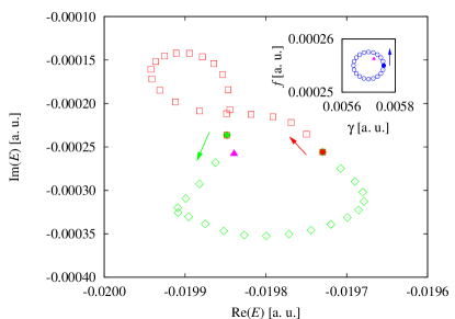
Figure 2: (Color online) Paths of the two eigenvalues (represented by squares and diamonds, respectively) which degenerate at the exceptional point labeled 14 in Table 1 in the complex energy plane Cartarius et al. (2007). Each point of one eigenvalue belongs to a different set of parameters. The path in the field strength parameter space is a circle defined in Eq. (14) with $\delta=0.01$ (see inset). The initial set of parameters and the corresponding eigenvalues are represented by filled starting points. The arrows indicate the direction of progression. The filled triangle marks the position of the exceptional point in the parameter space and the corresponding complex energy of the degenerate resonances.

shows a typical result obtained in a numerical calculation for the exceptional point labeled 14 in Table 1. The squares and the diamonds represent each of the eigenvalues at different field strengths. In this example, using 20 steps on the circle in the parameter space has been sufficient to obtain a clear signature of the branch point singularity. The “radius” of the circle according to Eq. (14) was $\delta=0.01$.

V Description of the resonance energies in the vicinity of exceptional points

V.1 Effective two-dimensional matrix

The most common case of an exceptional point consists of two resonances forming a square root branch point, whose effects on the spectrum appear in a close vicinity of the critical parameter values. There, only the two resonances involved in the branch point singularity are important if they are sufficiently separated from all further resonances, which in general can be realized since only a narrow region of the complex energy plane around two almost degenerate eigenvalues must be taken into account. In this case, one can restrict the discussion to the subspace spanned by the two relevant eigenvectors close to the exceptional point, which leads to effective two-dimensional matrix models. Indeed, two-dimensional models with only one complex parameter similar to the model introduced in Sec. II.2 yield a good description of the two complex eigenvalues in the vicinity of exceptional points Heiss (1999), and they can also provide good results for the resonances of the hydrogen atom in external fields. However, for some effects the actual matrix structure, which includes the two real field strengths $\gamma$ and $f$, has to be taken into account. We introduce a model adequate to describe the physical crossed-fields system. It is given by a matrix, whose elements have the form

$$M_{ij}=a^{(0)}_{ij}+a^{(\gamma)}_{ij}(\gamma-\gamma_{0})+a^{(f)}_{ij}(f-f_{0})\;,\quad i,j\in\{1,2\}\;.$$ (15)

This two-dimensional matrix is still a very simple model because it includes only the two states merging at the exceptional point and ignores couplings to other levels. Furthermore, a linear dependence of the matrix elements on the two field strengths is assumed, which is certainly only true for small distances to the center point $(\gamma_{0},f_{0})$. In contrast with the simple model used in Sec. II.2 it includes two real parameters with complex prefactors $a^{(0)}_{ij}$, $a^{(\gamma)}_{ij}$, $a^{(f)}_{ij}$ and correctly reproduces the matrix shape of the full Hamiltonian to lowest order. In a power series expansion its eigenvalues fulfill the relations

$$\lambda_{1}+\lambda_{2} =\mathrm{tr}(\bm{M})=A+B(\gamma-\gamma_{0})+C(f-f_{0})\;,$$ (16a)

$$(\lambda_{1}-\lambda_{2})^{2} =\mathrm{tr}(\bm{M})^{2}-4\mathrm{det}(\bm{M})=D+E(\gamma-\gamma_{0})$$

$$\quad+F(f-f_{0})+G(\gamma-\gamma_{0})^{2}$$

$$\quad+H(\gamma-\gamma_{0})(f-f_{0})+I(f-f_{0})^{2}$$ (16b)

with new coefficients $A$, $B$, $C$, $D$, $E$, $F$, $G$, $H$, and $I$. Since the eigenvalues do not change under a similarity transformation of the matrix $\bm{M}$ and the explicit choice of the matrix is not relevant, the representation (16a) and (16b) is more suitable than Eq. (15), in which more coefficients appear. The coefficients can be determined by a fit of the exact quantum energies to Eqs. (16a) and (16b) in a region of the parameter space in which only two resonances are relevant. A fit for 6 different parameter sets yields the 9 coefficients $A$ to $I$ and, thus, determines completely the two eigenvalues of the model (15) in dependence of the deviations from the center point $(\gamma_{0},f_{0})$. Six differences $\lambda_{1}-\lambda_{2}$ are required to determine $D$, $E$, $F$, $G$, $H$, and $I$. Three of the same parameter sets can be used to determine $A$, $B$, and $C$ from the sum $\lambda_{1}+\lambda_{2}$.

V.2 Shapes of the eigenvalue loops

As can be seen in Fig. 2 the shape of the paths covered by the two energy eigenvalues differs considerably from the semicircle form obtained for a small loop in the simple two-dimensional matrix model in Fig. 1(b). A good description of the complicated behavior is possible with the model (16a), (16b). The results of a more detailed investigation of the phenomenon with the matrix model are shown in Fig. 3.

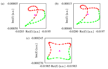
Figure 3: (Color online) Paths of the two eigenvalues considered in Fig. 2 for different radii of the parameter space circle (14), where the center $(\gamma_{0},f_{0})=(\gamma^{\mathrm{(EP)}},f^{\mathrm{(EP)}})$ was always chosen to be exactly the exceptional point. (a) $\delta=3\times 10^{-2}$, (b) $\delta=10^{-2}$, (c) $\delta=10^{-4}$. The position of the resonances at $(\gamma^{\mathrm{(EP)}},f^{\mathrm{(EP)}})$ is marked by a triangle in each figure. The squares and diamonds represent the exact quantum resonances. The lines represent the eigenvalues of the two-dimensional matrix model (15), whose coefficients have been fitted to the numerical results of the exact quantum calculations.

A circle around the exceptional point, which is always located exactly at the center of each figure, is performed for three different radii. For radii $\delta=0.03$ and $\delta=0.01$ (see Figs. 3(a) and (b)) the complicated structure already known from Fig. 2(a) appears. The deformations of the eigenvalue paths can be reproduced with the matrix (15). The lines in Figs. 3(a) and (b) represent the positions of the two model eigenvalues $\lambda_{1}$ and $\lambda_{2}$ for the same parameter space circle which was used for the exact quantum resonances. The very good agreement demonstrates that it is possible to describe the local structure of the resonances at an exceptional point with a simple two-dimensional model that ignores the influence of further resonances even if complicated structures in the eigenvalue paths appear.

Fig. 3(c) shows a circle around the same exceptional point for the much smaller radius $\delta=10^{-4}$, where the shape of the paths becomes more similar to the semicircle known from Fig. 1(b). The exceptional point marked by the triangle in Fig. 3(c) now is located at the center of the enclosing eigenvalue trajectories. However, the loop still is not a perfect semicircle. This effect is a result of the dependence on two real parameters with two complex prefactors as introduced in the model (15). While the models using one complex parameter (cf. Sec. II.2) lead to a perfect semicircle, as was demonstrated with the power series expansion (4), this is not the case for the description (15). A short calculation shows that a fractional power series expansion similar to Eq. (4) for the model (16a), (16b) to lowest order reads

$$\lambda_{1,2}=\begin{cases}\frac{A}{2}\pm\frac{1}{2}\sqrt{\frac{U}{2}\delta}\;\sqrt{1+\frac{V}{U}\mathrm{e}^{-\mathrm{i}2\varphi}}\;\mathrm{e}^{\mathrm{i}\varphi/2}\;,&\text{if }|V|<|U|\\ \frac{A}{2}\pm\frac{1}{2}\sqrt{\frac{V}{2}\delta}\;\sqrt{1+\frac{U}{V}\mathrm{e}^{\mathrm{i}2\varphi}}\;\mathrm{e}^{-\mathrm{i}\varphi/2}\;,&\text{if }|V|>|U|\end{cases}$$ (17)

with $U=E\gamma_{0}+Ff_{0}$, and $V=E\gamma_{0}-Ff_{0}$. The second term under the second square root is large enough to have a considerable influence and leads to the modulation of the “radius” during the traversal of the semicircle evident in Fig. 3(c). Again, the model fitted to the numerical data, and rendered by the continuous lines in the figure, perfectly reproduces the exact behavior.

Intersections of an eigenvalue path with itself are observed, which means that the eigenvalue can have the same complex energy for two different parameter sets. In Fig. 3(a) one can even see that the position of the exceptional point lies outside the area enclosed by the two eigenvalue paths. This is possible if one of the two eigenvalues (in this example obviously the resonance denoted by red squares) has the same complex energy as the one at the exceptional point for a second parameter set. The crossing of an eigenvalue path with the position of an exceptional point in the complex energy plane is shown in Fig. 4.

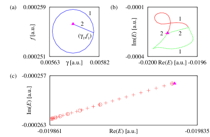
Figure 4: (Color online) (a) A circle in the parameter space (labeled 1) is chosen such that it passes through the parameter set $(\gamma_{1},f_{1})$ at which one of the energy eigenvalues is identical with its position at the exceptional point. A straight line (labeled 2) connects the parameters of the exceptional point and the parameter set $(\gamma_{1},f_{1})$. (b) Paths of the two numerically exact complex energies for the circle and the straight line described in (a). (c) Magnification of the path of the eigenvalue denoted by the red solid line in (b) for the parameter line labeled 2 in (a). The eigenvalue departs from the point of degeneracy (circles) and returns to its initial value (plus symbols).

The parameter space circle labeled 1 in Fig. 4(a) is chosen such that it passes directly through the point $(\gamma_{1},f_{1})$ at which one of the resonances returns to its initial position at the exceptional point as can be seen in Fig. 4(b). Additionally, the straight line labeled 2 in Fig. 4(a) is traversed. For this line one observes that both resonances leave the position of the exceptional point. The resonance denoted by the solid red line returns to its original position on the same path as can be seen in the magnified illustration in Fig. 4(c).

VI Dipole matrix elements and the photoionization cross section at exceptional points

In the correct inner product, which has to be used for the complex rotated states, no complex conjugation of the factors $\mathrm{e}^{\mathrm{i}\theta}$ (cf. Eq. (9)) may be performed Moiseyev (1998). Only the intrinsic complex parts of the wave functions are complex conjugated. An important consequence is that resonance wave functions normalized with respect to this inner product diverge at the branch points, which is typical of exceptional points Heiss (1999). In the simple two-dimensional matrix model introduced in Sec. II.2 that behavior can be observed directly for the normalized eigenvectors

$$\bm{x}_{1,2}(\kappa)=\frac{1}{\sqrt{\kappa^{2}+\left(1\mp\sqrt{1+\kappa^{2}}\right)^{2}}}\left(\begin{array}[]{c}-\kappa\\ 1\mp\sqrt{1+\kappa^{2}}\end{array}\right)$$ (18)

at the exceptional points $\kappa=\pm\mathrm{i}$.

One may wonder whether or not the diverging behavior carries over to measurable physical quantities. In particular, the photoionization cross section is important for the observation of resonances in experiments. For example, in Ref. Cartarius et al. (2007) it was proposed to measure the photoionization cross section for parameter sets located on a closed curve and to extract the complex energies of the resonances from the cross section with the harmonic inversion method. This procedure allows for searching the permutation behavior in experimental data.

As presented by Rescigno and McKoy Rescigno and McKoy (1975) the dipole matrix elements

$$P_{j}(E)=\langle\Psi_{0}|D(\bm{r})|\Psi_{j}(\theta)\rangle$$ (19)

and the photoionization cross section

$$\sigma(E)=4\pi\alpha_{\mathrm{elm}}(E-E_{0})\mathrm{Im}\left(\sum_{j}\frac{\left<\Psi_{0}|D|\Psi_{j}(\theta)\right>^{2}}{E_{j}-E}\right)\;,$$ (20)

can straightforwardly be calculated once the energies obtained from the complex rotated Hamiltonian and the corresponding eigenvectors are at hand. In Eq. (20) $D$ is the dipole operator in atomic units for a given direction of polarization and $\alpha_{\mathrm{elm}}$ is the fine-structure constant. The bound state, whose energy $E_{0}$ is supposed to be known, is represented by $\Psi_{0}$. The ionized states are labeled $\Psi_{j}$, where the rotated eigenfunctions calculated by the complex rotation method are used. In converged spectra, the result is independent of $\theta$.

Due to the dependence of Eqs. (19) and (20) on the resonance wave functions $\Psi_{j}$ a remarkable behavior at exceptional points occurs. The diverging behavior of the wave functions must carry over to the dipole matrix elements and, indeed, the numerical results show that the resonance wave functions obtained by the complex rotation method lead to diverging dipole matrix elements. This is, however, not an observable physical property because the single dipole matrix elements of the two identical wave functions at an exceptional point are not accessible. In particular, the photoionization cross section behaves regularly and does not diverge at an exceptional point as will be shown below.

Again, a two-dimensional matrix model helps in understanding these effects. To keep the discussion transparent, the simplest example, namely the symmetric matrix model introduced in Sec. II.2 is used, the results, however, are valid for all complex symmetric matrices. Note that in particular there is no difference visible in the behavior of the eigenvalues between the lowest-order power series expansions (4) and (17) if only the distance $\delta$ (or $\varrho$) is varied and the angle $\varphi$ is kept constant. The normalized eigenvectors, which correspond to the resonance wave functions $\Psi_{j}$, in this model are given by Eq. (18). The form of the dipole matrix elements (19) is represented by a product $P_{1,2}=\bm{y}\cdot\bm{x}_{1,2}$ of the eigenvectors $\bm{x}_{1,2}$ with an arbitrary vector $\bm{y}=(y_{1},y_{2})$. If the squares of the dipole matrix elements, which are required for the photoionization cross section, are calculated for a small complex deviation $\delta$ from one of the two exceptional points, $\kappa=\mathrm{i}+\delta$, a fractional power series expansion shows that the single contributions

$$\bar{P}_{1,2}^{2}=(\bm{y}\cdot\bm{x}_{1,2})^{2}=\pm\frac{\mathrm{e}^{\mathrm{i}3\pi/4}}{2\sqrt{2}}\frac{(y_{1}+\mathrm{i}y_{2})^{2}}{\sqrt{\delta}}+\frac{1}{2}(y_{1}^{2}+y_{2}^{2})\\ \pm\frac{\mathrm{e}^{\mathrm{i}5\pi/4}}{8\sqrt{2}}(y_{1}^{2}-6\mathrm{i}y_{1}y_{2}-y_{2}^{2})\sqrt{\delta}+\mathrm{O}(\delta)$$ (21)

diverge as $1/\sqrt{\delta}$. It is interesting to note that the sum of both contributions always has the exact value

$$(\bm{y}\cdot\bm{x}_{1})^{2}+(\bm{y}\cdot\bm{x}_{2})^{2}=y_{1}^{2}+y_{2}^{2}\;,$$ (22)

independent of the parameter $\kappa$, i.e., of the presence of the exceptional point, and of the matrix used. What is more interesting, however, is the sum

$$\bar{\sigma}=\frac{(\bm{y}\cdot\bm{x}_{1})^{2}}{\lambda_{1}-E}+\frac{(\bm{y}\cdot\bm{x}_{2})^{2}}{\lambda_{2}-E}\;,$$ (23)

which describes the contribution of the two resonances to the photoionization cross section with the eigenvalues (2) and a real variable $E$ representing the energy. Here, one can also look at the contributions of the single eigenvalues, and obtains in a fractional power series expansion around the branch point

$$\bar{\sigma}_{1,2}=\frac{(\bm{y}\cdot\bm{x}_{1,2})^{2}}{\lambda_{1,2}-E}=\pm\frac{\mathrm{e}^{\mathrm{i}7\pi/4}}{2\sqrt{2}}\frac{(y_{1}+\mathrm{i}y_{2})^{2}}{E\sqrt{\delta}}+f_{1}(E,\bm{y})\\ \pm f_{2}(E,\bm{y})\sqrt{\delta}+f_{3}(E,\bm{y})\delta+\mathrm{O}(\delta^{3/2})$$ (24)

with rather complicated expressions $f_{1}(E,\bm{y})$, $f_{2}(E,\bm{y})$, and $f_{3}(E,\bm{y})$ which do not depend on $\delta$. These parts diverge, however, $\bar{\sigma}_{1}$ and $\bar{\sigma}_{2}$ alone are not observable. The sum contributes to the photoionization cross section, and, in particular, at the exceptional point ($\delta=0$) the two resonances overlap. For the sum one finds

$$\bar{\sigma}=2f_{1}(E,\bm{y})+2f_{3}(E,\bm{y})\delta+\mathrm{O}(\delta^{2})\;,$$ (25)

that is, the photoionization cross section converges linearly to a constant value at the branch point.

Numerical calculations for the hydrogen spectra discussed in this paper

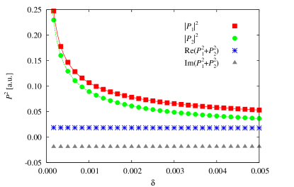
Figure 5: (Color online) Squares $P^{2}$ of the dipole matrix elements between a wave function corresponding to a bound state and the two states evolving from the exceptional point labeled 12 in Table 1 at field strengths according to the form (14) with the constant angle $\varphi=0.7$ and $(\gamma_{0},f_{0})=(\gamma^{\mathrm{(EP)}},f^{\mathrm{(EP)}})$, $\delta$ is the distance from the critical values of the exceptional point. For both states the square modulus diverges in the form of a reciprocal square root of the distance. A fit of the data points to a function of the form $a/\sqrt{\delta}+b$, which is expected from Eq. (21), is shown by the solid red and dashed green lines. The real and the imaginary part of the sum $P_{1}^{2}+P_{2}^{2}$ is also drawn.

demonstrate the applicability of the simple model. For this purpose, the square modulus of the dipole matrix elements (19) and the photoionization cross section (20) are calculated on a straight line of the form (14) for a constant angle $\varphi$ and variable distance $\delta$ from the exceptional point $(\gamma_{0},f_{0})=(\gamma^{\mathrm{(EP)}},f^{\mathrm{(EP)}})$. The results have been verified for different angles $\varphi$. Fig. 5 shows the squares of the two isolated dipole matrix elements for the resonances which form the exceptional point labeled 12 in Table 1. Both matrix elements behave as predicted by the approximation (21) of the simple two-dimensional model. The single terms $|P_{1}|^{2}$ and $|P_{2}|^{2}$ diverge in the form of a reciprocal square root of $\delta$ which is shown by a fit of the numerical results to the function

$$P_{\mathrm{fit}}(\delta)=\frac{a}{\sqrt{\delta}}+b\;.$$ (26)

An excellent agreement can be observed. Additionally, the real and imaginary parts of the sum $P_{1}^{2}+P_{2}^{2}$ are plotted. As expected from Eq. (22) for the two-dimensional model, this sum has a constant value.

The photoionization cross section $\sigma(\mathrm{Re}(E^{\mathrm{(EP)}}))$ evaluated at the real part of the energy $E^{\mathrm{(EP)}}$ at the exceptional point according to Eq. (20) is shown in Fig. 6 as a function of the distance parameter $\delta$.

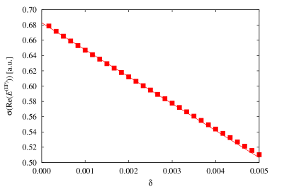
Figure 6: (Color online) Photoionization cross section $\sigma(\mathrm{Re}(E^{\mathrm{(EP)}}))$ with the bound state energy $E_{0}=-0.125$ ($n=2$, p-orbital) as a function of the distance $\delta$ from the critical field values of the exceptional point. The numerical data (dots) converge linearly to a constant value as is expected from Eq. (25). Again, the line (14) with constant angle $\varphi=0.7$ and $(\gamma_{0},f_{0})=(\gamma^{\mathrm{(EP)}},f^{\mathrm{(EP)}})$ is used.

As can be seen directly in the figure the numerical data points (red points) converge linearly to a constant value for $\delta\to 0$. The red line represents a fit to the function

$$\sigma_{\mathrm{fit}}(\mathrm{Re}(E^{\mathrm{(EP)}}))=a+b\delta$$ (27)

whose form is expected from the power series expansion (25) of the two-dimensional model. The comparison shows an excellent agreement.

VII Structures with three resonances

Beyond the typical square root branch point behavior studied in most physical examples, higher branch points connecting more than two eigenvalues are possible. In particular, the possibility of a cubic root branch point in a three-dimensional symmetric matrix is the topic of current studies Heiss (2008). For a complex symmetric matrix a coalescence of $N$ levels requires $(N^{2}+N-2)/2$ real parameters Heiss (2008). Thus, for $N=3$ five parameters are necessary. For the hydrogen atom this means that additionally to the two field strengths $\gamma$ and $f$ three further parameters have to be introduced. Locating exceptional points in a five-dimensional parameter space is expected to be a laborious task considering the difficulties encountered already for two parameters. However, as will be shown below, a combination of three resonances strongly related to a cubic root branch point is observable in spectra of the crossed-fields hydrogen atom. In particular the permutation behavior of a cubic root branch point, where three resonances are permuted and three circles in the parameter space are required to restore the original situation, can be found.

An example where three resonances come into play is given in Fig. 7.

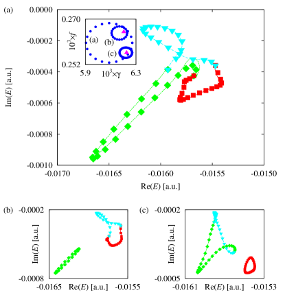
Figure 7: (Color online) Illustration of a structure in the vicinity of two exceptional points in which three resonances are involved. Each of the resonances is denoted by a different symbol and color. The inset of Fig. (a) shows the three parameter space loops (circles) and the position of the two exceptional points (up triangles). In Fig. (a) the parameter space loop (indicated by dots) is chosen such that both exceptional points are located within the circular area. The resonance marked by down triangles forms a branch point singularity with two further states at two different parameter values, which is shown by two additional parameter space loops (small circles in the inset) in whose circular area only one of the two exceptional points is located (Figs. (b) and (c)). The solid lines mark the eigenvalues of the three-dimensional model (28b)-(28d) fitted to the numerical data.

In Fig. 7(a) obviously a permutation of three eigenvalues indicated by points with three different symbols and colors can be observed for a closed loop in the parameter space. From that behavior one might assume that indeed an exceptional point consisting of three resonances, which form a cubic root branch point singularity, was detected. A more detailed analysis shows, however, that this is not the case. But there is a close relationship with a triple coalescence. There are two exceptional points located in the circular area of the parameter space circle of the type (14) used in Fig. 7(a). This can directly be shown if one chooses two different parameter loops with two different center points $(\gamma_{0},f_{0})$ and smaller radii $\delta$, which is done in Figs. 7(b) and (c). Then one observes that there are two exceptional points at which two of the three resonances form a square root branch point. The resonance denoted by down triangles in Fig. 7 is involved in both exceptional points. For the large parameter space circle used for Fig. 7(a) the two different exceptional points cannot be resolved and the eigenvalue paths form the permutation of three resonances which looks like a triple coalescence in the form of a cubic root branch point. Although no exact triple coalescence was found the finding of the situation depicted here is already a remarkable result. Two exceptional points located close to each other in the parameter space are required. Furthermore, only three resonances may be connected with these exceptional points, i.e., one of them must be connected with both branch points. If three additional parameters were available, a coalescence of both exceptional points would be possible or, in other words, the additional parameters would be necessary to shift the three resonances such that they form a cubic root branch point in the five-dimensional parameter space.

Of course, it is not possible to describe a behavior of this kind with the two-dimensional matrix models used so far. At least a three-dimensional model is required to simulate three energy eigenvalues connected with each other. Indeed, it can be shown that it is possible to reconstruct the structures shown in Fig. 7 by a three-dimensional matrix model. Similar to the ansatz (15) we expand the matrix elements in a power series in the two field strengths $\gamma$ and $f$ around a center point, and specifically assume the matrix to be symmetric. To model the behavior of its eigenvalues $\lambda$, we fit the coefficients of the characteristic polynomial

$$\lambda^{3}+a\lambda^{2}+b\lambda+c=0$$ (28a)

to the exact numerical results. Note that one has the familiar relations

$$a =-(\lambda_{1}+\lambda_{2}+\lambda_{3})\;,$$ (28b)

$$b =\lambda_{1}\lambda_{2}+\lambda_{1}\lambda_{3}+\lambda_{2}\lambda_{3}\;,$$ (28c)

$$c =-\lambda_{1}\lambda_{2}\lambda_{3}\;.$$ (28d)

For the discussion in Fig. 7 a power series expansion of the coefficients $a$, $b$, and $c$ up to third order in both field strengths was included, which leads to 30 terms for all three coefficients, i.e., 10 combinations of field strengths are required to obtain 10 triples of eigenvalues for the relations (28b)–(28d). The eigenvalues in the three-dimensional matrix model are shown as solid lines in Figs. 7(a), (b), and (c) and agree very well with the numerically exact resonances. This shows that it is sufficient to only take the three resonances into account to explain their behavior. The influence of further resonances can be ignored in the investigation of the threefold permutation. The model can even be used to predict the positions of the two exceptional points located within the parameter space loop. For the case shown in Fig. 7(a) the model predicts the positions of the two exceptional points labeled 15 and 16 in Table 1 at $(\gamma_{1}=6.12\times 10^{-3},f_{1}=2.53\times 10^{-4})$ and $(\gamma_{2}=6.15\times 10^{-3},f_{2}=2.68\times 10^{-4})$, respectively, which well approximates the results of the full quantum treatment.

VIII Connection with avoided level crossings

There is a close relation between avoided level crossings of the real energies of bound states and exceptional points. As has been demonstrated, the level repulsions of bound states of a Hermitian Hamiltonian which depends on one real parameter are associated with an exceptional point if the parameter is continued into the complex plane Heiss and Sannino (1990); Heiss (1999). A similar effect appears with resonances of open quantum systems. Here one can observe crossings or avoided crossings of either the positions or the widths of the resonances for lines in the parameter space which do not run over the exceptional point. This behavior has, e.g., been discussed for the resonances in microwave cavities Dembowski et al. (2001).

Avoided level crossings of the energies or widths can also be observed in spectra of the hydrogen atom in external fields. Fig. 8 shows the real part of the complex energy as a function of a parameter $\alpha$ which defines a straight line of the form

$$\gamma =0.80516\times 10^{-2}\alpha\;,$$ (29a)

$$f =0.32169\times 10^{-3}\alpha\;,$$ (29b)

$$\gamma/f =25.03$$ (29c)

in the $(\gamma,f)$-space.

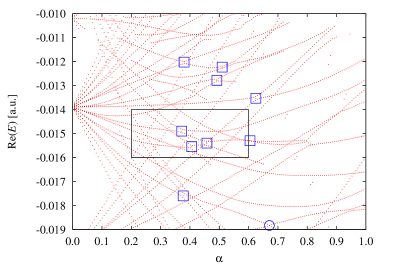
Figure 8: (Color online) Real part of the complex energy as a function of the one-dimensional parameter $\alpha$, $\gamma=0.80516\times 10^{-2}\alpha$, $f=0.32169\times 10^{-3}\alpha$, defined in Eqs. (29a) and (29b). The blue circle marks an exceptional point. Avoided crossings (marked by blue squares) appear, which are related to exceptional points. Only resonances with $|\mathrm{Im}(E)|<0.0005$ are drawn to not overload the figure. The black frame marks the region investigated in detail in Fig. 9(a) to demonstrate how an avoided crossing leads to an exceptional point if the parameters are varied.

The line is chosen such that it passes directly through the exceptional point labeled 12 in Table 1. The position of the exceptional point is marked by the blue circle in the figure. In the vicinity of the parameter space line further exceptional points are located. Since the line does not pass through these critical parameter values, the exceptional points only manifest themselves by avoided crossings in the energies or the widths. The avoided energy (real part) crossings are shown in the figure. They are marked by blue squares. The close connection between avoided crossings and branch point singularities of exceptional points can be shown very directly. In all cases marked in Fig. 8 it is possible to vary the parameters $\gamma$ and $f$ such that a coalescence of the two eigenvalues forming the avoided crossing is achieved. That is, all avoided crossings shown in the diagram are associated with exceptional points of the corresponding resonances. In all cases where the description of the energy range under consideration is possible with the model (15), i.e., always if only two resonances are involved, the adjustment of the parameters $\gamma$ and $f$ leads to a branch point. In other words, exceptional points are indeed found to be the origin of narrow avoided level crossings.

A more detailed illustration is given in Fig. 9.

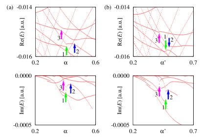
Figure 9: (Color online) (a) Detailed illustration of the region marked by the black frame in Fig. 8. Three avoided energy crossings are present. In addition, the imaginary part is shown, which exhibits two crossings (arrows 1 and 3) and one avoided crossing (arrow 2). (b) The same region is shown for the field strengths varied on the line $\gamma=0.65378\times 10^{-2}\alpha^{\prime}$, $f=0.28213\times 10^{-3}\alpha^{\prime}$ given by Eqs. (30a) and (30b). One of the three exceptional points is located on this line and the corresponding avoided energy crossing marked by arrow 3 has been transformed into a branch point singularity, where both the real and imaginary parts are identical. The other two encounters show at least one avoided crossing in the real or in the imaginary part.

The region marked by the black frame in Fig. 8 is magnified in Fig. 9(a). Three of the avoided level crossings are included and, in addition, the imaginary part of the resonances is shown. The encounter of two resonances marked by the arrow labeled 1 shows an avoided crossing in the real part and a crossing in the imaginary part. The arrow 2 exhibits avoided crossings in the real as well as in the imaginary part. The encounter marked by arrow 3 shows an avoided crossing of the real part which is accompanied by a crossing in the imaginary part. Its behavior changes on a neighboring line in the parameter space defined by

$$\gamma =0.65378\times 10^{-2}\alpha^{\prime}\;,$$ (30a)

$$f =0.28213\times 10^{-3}\alpha^{\prime}\;,$$ (30b)

$$\gamma/f =23.17\;.$$ (30c)

Now the avoided energy crossing is changed into a crossing, which can be seen in Fig. 9(b). The line (30a), (30b) runs exactly through the corresponding exceptional point. As a consequence the avoided crossing is transformed into a branch point degeneracy at which both the real and imaginary parts are identical, whereas the other two encounters do not form a degeneracy. They belong to different exceptional points which are not hit by the line. The encounter labeled by arrow 2 forms, again, an avoided crossing both in the real and in the imaginary part. The third encounter, which is marked by arrow 1 has inverted its behavior. Now, it forms a real part crossing and an avoided crossing of the imaginary part.

The connection between avoided crossings and exceptional points provides an additional possibility of detecting the branch point singularities in spectra of the hydrogen atom in external fields. Exceptional points can be found by plotting the real part of the complex resonance energies as a function of one parameter, similar to $\alpha$ in Eqs. (29a) and (29b). If avoided crossings of the energy are found, the identification of the exceptional point can be performed by the method presented in Sec. IV.1.

IX Conclusion and outlook

Exceptional points are a feature that can emerge in parameter-dependent open quantum systems with decaying unbound states. They are branch point singularities at which two eigenstates of a non-Hermitian Hamiltonian coalesce. The topic of this paper was to investigate these exceptional points in the spectra of atoms in external fields. It has been shown, that the branch point singularities can be found by the permutation of two eigenvalues when an exceptional point is encircled in the parameter space. This method works reliably.

The effects of exceptional points on spectra of the hydrogen atom in external fields have been analyzed in detail. In a close region around the branch points, it is possible to describe the two branching eigenstates by $2\times 2$-matrix models and to explain the structure of the loops the eigenvalues traverse for closed paths in the parameter space. The study of dipole matrix elements in the vicinity of branch points has revealed remarkable properties. While single dipole matrix elements diverge in the presence of exceptional points this is not the case for observable physical quantities such as the photoionization cross section. Both behaviors can be explained by a simple matrix model, which provides an excellent qualitative description of the properties in the local vicinity of the branch point singularity.

Beyond the typical square root branch points the spectra of the hydrogen atom exhibit structures in which three resonances are connected via two exceptional points. One of the three resonances is involved in both branch points. This finding is especially important because it is closely related to a cubic root branch point, at which all three resonances coalesce. The direct adjustment of such a cubic root branch point would require five external parameters and therefore is not possible in the system investigated here. Furthermore, the close relation of avoided level crossings and exceptional points could be confirmed in the resonances of the hydrogen atom in external fields.

As an outlook, it should be possible to extend the two-dimensional matrix model introduced in this paper to develop a further, and possibly very fast, method to determine the exact position of an exceptional point. Once its existence has been detected by the permutation of two eigenvalues the fit to the two-dimensional matrix model can be used to predict the position of the degeneracy in parameter space by solving Eq. (16b) for $\lambda_{1}=\lambda_{2}$ which is a very easy task. The improved position of the exceptional point can be used to perform a smaller parameter space circle and to apply the procedure iteratively.

With the procedure proposed in Ref. Cartarius et al. (2007) it should be possible to verify experimentally the effects of exceptional points on the spectra of atoms in external fields discussed in this paper. In particular, the permutation behavior to prove their existence, the influence on the photoionization cross section, and the close relation to avoided level crossings should be observable.