Magnetization of Two Dimensional Heavy Holes with Boundaries in a Perpendicular Magnetic Field

Abstract

The magnetization of heavy holes in III-V semiconductor quantum wells with Rashba spin-orbit coupling (SOC) in an external perpendicular magnetic field is theoretically studied. We concentrate on the effects on the magnetization induced by the system boundary, the Rashba SOC and the temperature. It is found that the sawtooth-like de Haas–van Alphen (dHvA) oscillations of the magnetization will change dramatically in the presence of such three factors. Especially, the effects of the edge states and Rashba SOC on the magnetization are more evident when the magnetic field is more small. The oscillation center will shift when the boundary effect is considered and the Rashba SOC will bring beating patterns to the dHvA oscillations. These effects on the dHvA oscillations are preferred to be observed at low temperature. With increasing the temperature, the dHvA oscillations turn to be blurred and eventually disappear.

I Introduction

The physics of low dimensional electron systems in high magnetic fields is one of the most important subjects of semiconductor physics. Recently, great attentions are taken to the magnetic properties of two dimensional (2D) systems in a strong perpendicular magnetic field both experimentally and theoreticallyZhu et al. (2003); Schaapman et al. (2003); Gudmundsson et al. (2000); Niţá M et al. (2000); Harris et al. (2001). Such systems are candidates for next-generation spintronic devicesOhno (1998); Wolf et al. (2001); Gupta et al. (2001) because of their very high electron mobility compared with silicon. In the absence of disorder and interactions, due to the Landau energy quantization in an external magnetic field, the magnetization is predicted to oscillate periodically in a sawtooth pattern as a function of $B$ or filling factor $\nu$, which is the famous de Haas– van Alphen (dHvA) oscillationPeierls (1933); Vagner et al. (1983); Shoenberg (1984). The dHvA oscillation is a powerful tool used extensively to determine the electronic properties of bulk semiconductors and metals, such as Fermi surface geometry and effective masses. It has been evident now that the magnetization, which turns to be zero for classical electrons, appears due to the presence of the sample boundaryL. Bremme and Ensslin (1999), the spin orbital coupling (SOC) or Zeeman splitting. Once a perpendicular magnetic field was applied, these factors would change the magnetization dramatically. Firstly, in a finite size sample with boundaries the edge states play important roles in quantum transport in high magnetic fields, such as quantum Hall effect or magneto-tunneling effect. From the semiclassical point of view when electrons are located near the edge of the samples, cyclotron motion cannot fulfill the entire cyclotron orbit if the distance between the center of the cyclotron orbit and the edge is smaller than the radius of the cyclotron motion. In such a case, the electron orbit is bounced at the edge plane, and the bounced electrons conduct a one-dimensional motion as a whole being repeatedly reflected at the edge plane, resulting a skipping orbit. The edge states with a skipping orbit are different from those in the interior of the sample where the cyclotron orbit is completed. Although these edge states are localized in the vicinity of the confining walls, the measurable bulk quantities are completely modified by the edge states, certainly including the magnetization. Secondly, the Rashba SOC, competed with the Landau splitting and the Zeeman splitting, will modulate the energy spectrum. As a result, the Rashba SOC will have non-neglectable influence on the dHvA oscillations of the magnetization.

However, to our knowledge there are no detailed treatments on the influence of edge states and SOC on the magnetization in 2D systems, except for the 2D electron systems much recently studied by our groupWang et al. . In this paper, we study systematically the thermodynamic magnetization of heavy holes in III-V semiconductor quantum wells with boundaries in the presence of the Rashba SOC due to structure-inversion asymmetry, with an external magnetic field applied perpendicularly. We will show that the dHvA oscillations of the magnetization change dramatically due to the presence of SOC and system boundaries. The edge states lead to the change of both the center and the amplitude of the sawtoothlike dHvA oscillations of the magnetization. The SOC mixes the spin-up and spin-down states of neighboring Landau Levels into two unequally spaced energy branches, which further changes the well-defined sawtoothlike dHvA oscillations of the magnetization. These effects on the magnetization can be observed at low temperature in experiment. With increasing the temperature, the dHvA oscillations of the magnetization turn to be blurred and eventually disappear.

This paper is organized as follows: Sec.II focuses on the quantum mechanical solution of the heavy-holes in III-V semiconductor quantum wells. Using numerical diagonalization of the Hamiltonian in a truncated Hilbert space we calculate the energy spectrum. Sec.III gives the main results of this paper on the magnetization and makes a detailed discussion. The last section gives a short summary.

II Energy spectrum of the heavy holes

Now we consider a 2D hole gas system in which a Rashba SOC arises from the quantum well asymmetry in the growth ($z$). The Hamiltonian for heavy holes in III-V semiconductor quantum wells within a perpendicular magnetic field $\mathbf{B}=-B\hat{e}_{z}$, taking into account the kinetic energy and the Zeeman magnetic field, can be written as

$$H=\frac{\Pi^{2}}{2m^{\ast}}+i\frac{\alpha}{2\hbar^{3}}\left(\Pi_{-}^{3}\sigma_{+}-\Pi_{+}^{3}\sigma_{-}\right)-\frac{3}{2}g_{s}\mu_{B}\mathbf{B}\sigma_{z}+V\left(y\right),$$ (1)

where $m^{\ast}$ being band effective mass, $\Pi_{\pm}=\Pi_{x}\pm i\Pi_{y}$ with $\Pi_{\eta}=\Pi_{\eta}+\left(e/c\right)A_{\eta}$, $\Pi_{\eta}$ and $A_{\eta}$ denoting the $\eta$ component of the momentum and vector potential, respectively. $\mathbf{B}$=$\nabla\times\mathbf{A}$. The Pauli matrices, $\sigma_{\pm}=\sigma_{x}\pm i\sigma_{y}$, operate on the total angular momentum states with spin projection $\pm 3/2$ along the growth direction; in this sense they represent a pseudospin degree of freedom rather than a genuine spin $1/2$Schliemann and Loss (2005). $\alpha$ is Rashba SOC coefficient due to structure inversion asymmetry across the quantum well grown along the $[001]$-direction chosen as the $z$-axis. For a symmetrically grown quantum well, the coefficient $\alpha$ is essentially proportional to an electric field applied across the well and therefore experimentally tunablePala et al. (2004a, b); Schliemann and Loss (2005); Winkler (2000); Winkler et al. (2002); Gerchikov and Subashiev (1992). $g_{s}$ is the gyromagnetic factor. The last term $V\left(y\right)$ is the lateral confining potential. For simplicity, a hard wall potential that confines the holes in the transverse $y$ direction is used,

$$V\left(y\right)=\begin{cases}0&0\leqslant y\leqslant L\\ \infty&\text{otherwise}\end{cases}.$$ (2)

It is convenient to use the Laudau gauge $\mathbf{A}=\left(yB,0,0\right)$ and to write the wave function in the form

$$\Psi\left(x,y\right)=e^{ikx}\psi\left(y\right)$$ (3)

with the function $\psi\left(y\right)$ expanded in the basis set of the infinite potential well,

$$\psi\left(y\right)=\sqrt{\frac{2}{L}}\sum_{n}\sin\left(\frac{\pi ny}{L}\right)\left(\begin{array}[]{c}a_{n}\\ b_{n}\end{array}\right).$$ (4)

Introducing the cyclotron center $y_{0}=-\frac{\hbar c}{eB}k=-l_{b}^{2}k$, the magnetic length $l_{b}=\sqrt{\hbar c/eB}$ and the cyclotron frequency $\omega_{c}=eB/m^{\ast}c$, the Schrödinger equation $H\Psi\left(x,y\right)=E\Psi\left(x,y\right)$ leads to the following equations for spinors:

$$\sum_{l}\left\{\left[M_{ln}-\hbar\omega_{c}\left(\frac{3}{2}g\sigma_{z}+\varepsilon\right)\delta_{ln}\right]+i\left[F_{ln}-G_{ln}\right]\sigma_{+}-i\left[F_{ln}+G_{ln}\right]\sigma_{-}\right\}\left(\begin{array}[]{c}a_{n}\\ b_{n}\end{array}\right)=0,$$ (5)

where

$$M_{ln} =\hbar\omega_{c}\frac{1}{\pi}\int_{0}^{\pi}\sin\left(lt\right)\left[\left(\frac{L}{\pi l_{b}}\right)^{2}\left(t-t_{0}\right)^{2}-\left(\frac{\pi l_{b}}{L}\right)^{2}\partial_{y}^{2}\right]\sin\left(nt\right)dt,$$

$$F_{ln} =\hbar\omega_{c}\frac{\eta}{L}\int_{0}^{\pi}\sin\left(lt\right)\left[3\partial_{t}+3\left(t-t_{0}\right)\partial_{t}^{2}+\left(\frac{L}{\pi l_{b}}\right)^{4}\left(t-t_{0}\right)^{3}\right]\sin\left(nt\right)dt,$$

$$G_{ln} =\hbar\omega_{c}\left(\frac{L}{\pi l_{b}}\right)^{2}\frac{\eta}{L}\int_{0}^{\pi}\sin\left(lt\right)\left[3\left(t-t_{0}\right)+3\left(y-y_{0}\right)^{2}\partial_{t}+\left(\frac{\pi l_{b}}{L}\right)^{4}\partial_{t}^{3}\right]\sin\left(nt\right)dt,$$

with $\varepsilon=E/\hbar\omega_{c}$,$\,\ t=\pi y/L$, $\,t_{0}=\pi y_{0}/L$, $g=m^{\ast}g_{s}/2m_{e}$, and $\eta=m^{\ast}\alpha l_{b}/\hbar^{2}$. Taking the same method in Ref.Reynoso et al. (2004), we solve the above equations in a truncated Hilbert space disregarding the highest energy states. Typically we take a matrix Hamiltonian of dimension of a few hundred. We increase the size of the Hilbert space by a factor $2$ and find no change in the results presented below. In all cases the width of the sample $L$ is taken large enough to have the cyclotron radius $r_{c}$ smaller than $L/2$. The right and left edge states are then well separated in real space. For $y_{0}\simeq L/2$ the states are equal to the bulk states, except for exponential corrections. The energy spectrum reproduces the bulk results without edge states, which is given by the follows:

$$\frac{E_{n}}{\hbar\omega_{c}}=\left(n-1\right)+\frac{3}{2}\left(1-g\right),\text{ \ \ }\left(n=0,1,2\right)$$ (6)

$$\frac{E_{n}}{\hbar\omega_{c}} = \left(n-1\right)+\frac{s}{2}\sqrt{4\gamma^{2}n\left(n-1\right)\left(n-2\right)+\left(3g-3\right)^{2}},$$ (7)

$$\hskip 156.49014pt\left(n\geq 3\right)$$

with $s$=$\pm 1$. The dimensionless parameter is defined by $\gamma=2\left(\alpha m^{\ast}/\hbar^{2}\right)\sqrt{2eB/\hbar c}$Ma and Liu (2006). As $y_{0}$ approaches the sample edge, the effect of the confining potential becomes important and it generates the $k$-dependent dispersion of the energy levels, which has profound effects on magnetotransport and magnetization properties. Fig.1 plots the the energy spectrum of the Hamiltonian (1) as a function of the cyclotron center $y_{0}$.

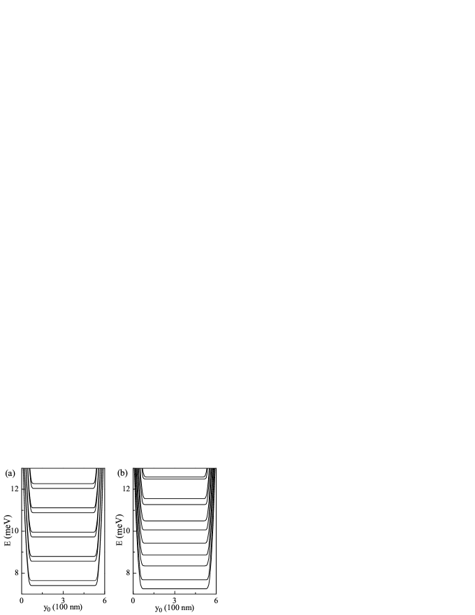
Figure 1: The energy spectrum in units of meV versus the guiding center $y_{0}$ without (a) and with (b) the Rashba SOC, respectively, for the 2D hole systems. In both figures, the effective mass $m^{\ast}$=$0.27m_{e}$, the system size $L$=$600\,$nm, the hole number density $N_{h}$=$0.01$ nm^-2, the magnetic field $B$=$3$T, and the $g$-factor $g_{s}$=$-0.44$.   The Rashba SOC strength in (b) is set as $\alpha$=$40\,$meV nm³. Clearly from (b) one can see that the introduced Rashba SOC mixes the the eigenstates of the spin operator $s_{z}$.

III The magnetization of the 2D holes

Now we investigate the magnetization of the 2D holes in the III-V semiconductor wells. According to the thermodynamics and the statistical physics, one easily obtains that the magnetization density is the derivative of the Helmholtz free energy density with respect to $B$ at fixed electron density $\mathcal{N}$ and temperature $T$, $M=-\left(\partial F/\partial B\right)|_{\mathcal{N},T}$. For the present 2D hole model, the free energy is given by

$$F(B,T) =\mu\mathcal{N}-\frac{1}{L}\frac{N_{\nu}}{\beta}\int_{0}^{L}\mathrm{d}y_{0}\sum_{n,s}\ln\left\{1+e^{\beta[\mu-E_{n,s}(y_{0})]}\right\}$$

$$\equiv\mu\mathcal{N}-\frac{1}{\beta}\int\mathrm{d}ED(E,B)\ln\{1+e^{\beta(\mu-E)}\},$$ (8)

where $\beta$=$1/k_{B}T$, $N_{\nu}$=$eB/hc$, and $\mu$ is the chemical potential. Note that we have defined in the above equation the density of states (DOS) per area

$$D(E,B)=\frac{N_{\nu}}{L}\sum_{n,s}\int_{0}^{L}\mathrm{d}y_{0}\delta(E-E_{n,s}(y_{0})).$$ (9)

The explicit inclusion of the DOS in the expression can be utilized to take into account the impurity effect, which broadens the Landau levels into Gaussian or Lorentzian in shape. For simplicity we do not consider the broadening effect in this paper. In the absence of edge states, the Landau Levels $E_{n,s}(y_{0})$ are uniform in space and thus Eq. (8) reduces to

$$F(B,T)=\mu\mathcal{N}-\frac{N_{\nu}}{\beta}\sum_{n,s}\ln\left\{1+e^{\beta(\mu-E_{n,s})}\right\}.$$ (10)

The $B$ dependent chemical potential $\mu$ is connected to the experimentally accessible electron density $\mathcal{N}$ via the local DOS. In the clean sample limit this is written as

$$\mathcal{N}=\frac{N_{\nu}}{L}\int_{0}^{L}\mathrm{d}y_{0}\sum_{n,s}f_{ns}\left(y_{0}\right),$$ (11)

where $f_{ns}\left(y_{0}\right)$=$\frac{1}{e^{\beta\left[E_{n,s}(y_{0})-\mu\right]}+1}$ is the Fermi distribution for the spin-split Landau levels $E_{n,s}(y_{0})$. From Eq. (8) the magnetization density becomes

$$M =\sum_{n,s}\left\{-N_{\nu}\int_{0}^{L}\frac{\mathrm{d}y_{0}}{L}f_{ns}\left(y_{0}\right)\frac{\partial E_{n,s}(y_{0})}{\partial B}\right.$$

$$\left.+\frac{e}{h}\frac{1}{\beta}\int_{0}^{L}\frac{\mathrm{d}y_{0}}{L}\ln\left\{1+e^{\beta\left[\mu-E_{n,s}(y_{0})\right]}\right\}\right\}$$

$$\equiv M^{(0)}+M^{(1)}.$$ (12)

One can see that the magnetization consists of two parts. The first part $M^{(0)}$ is the conventional contribution from the $B$ dependence of the Landau levels and thus is denoted as a paramagnetic response. The second part $M^{(1)}$ comes from the $B$ dependence of the level degeneracy factor $N_{\nu}$, thus describing the effect of the variation of the density of states upon the magnetic field. Obviously, $M^{(0)}$ is negative while $M^{(1)}$ is positive, the net result is an oscillation of the total magnetization $M$ between the negative and positive values as a function of $B$. At zero temperature, the expression for $M$ reduces to a sum over all occupied Landau levels:

$$M = \sum_{n,s}^{\text{occ}}\left\{-N_{\nu}\int_{0}^{L}\frac{\mathrm{d}y_{0}}{L}\frac{\partial E_{n,s}(y_{0})}{\partial B}\right.$$ (13)

$$\left.+\frac{e}{h}\int_{0}^{L}\frac{\mathrm{d}y_{0}}{L}[\mu_{0}-E_{n,s}(y_{0})]\right\},$$

where the sum runs over all occupied states and $\mu_{0}$ is the zero-temperature chemical potential (Fermi energy).

To clearly see the influence of the edge-states and Rashba SOC on the magnetization, let us begin with the conventional result for the bulk 2D holes without SOC and edge-state effects. In this case, the magnetization (per hole) $m$ (see the solid line in Fig. 2) displays the well-known sawtooth behavior with varying the magnetic field $B$. One fact revealed in Fig. 2 is that the inclusion of the Zeeman splitting in the Landau levels will result in many weak peaks appearing among the dHvA oscillation modes of the physical quantities, the chemical potential $\mu$ and the magnetization (per hole) $m$, at very low temperature (here $T=0.2$K). These weak peaks have been observed recently by Schaapman et alSchaapman et al. (2003) when they measured the magnetization of a dual-subband 2D electron gas, confined in a GaAs/AlGaAs heterojection, and by Zhu et alZhu et al. (2003) when they measured the magnetization of high-mobility 2D electron gas. From Fig. 2 one obtain that these weak peaks can also be observed in 2D hole system. These weak peaks will disappear when the temperature turns sufficiently high.

Figure 2: The dHvA oscillations of the magnetization (per hole) of 2D hole system with different system sizes. The parameters are chosen as follows: the effective mass $m^{\ast}$=$0.27m_{e}$, the hole number density $N_{h}$=$0.01$ nm^-2, the $g$-factor $g_{s}$=$-0.44$, and the temperature $T=0.5$K. The Rashba SOC here is neglected.

Then we investigate the edge-state effects on the magnetization. Fig. 2 (the dashed, dotted, and dash-dotted lines) also shows the influence of the edge states on the oscillations of chemical potential and magnetization (dHvA oscillations) with magnetic field. From Fig. 2 one can easily observe a prominent feature brought by the edge states, which is that the center of the dHvA oscillations is now dependent on the magnetic field. In particular, for the field less than $1$ Tesla, the oscillatory magnetization is always positive in sign. Another feature shown in Fig. 2 is that the oscillation amplitude decreases with decreasing the sample size. As is known, the origin of dHvA oscillations is the degeneracy of Landau levels. The edge states with dispersion lead to edge current, which not only is crucial for the quantum Hall effects, but also very important for the magnetization L. Bremme and Ensslin (1999). The dispersion of the edge states partially lift the degeneracy of the Landau levels. Thus the edge states tend to destroy the dHvA oscillations. Therefore it leads to the decreasing of oscillation amplitude as shown in Fig. 2. The upshift of the center of dHvA oscillations may be understood as follows: For the effects from the edge states, what really matters is the ratio of two important length scales: the magnetic length $l_{b}$ and the system size $L$. The decreasing of $L$ is equivalent to the increasing of $l_{b}$, i.e., decreasing of $B$ or $\omega_{c}$. From Eq. (12), one can see that with decreasing of $L$, the second term overcomes the first term and leads to the upshift of the center of dHvA oscillations. The smaller the system size is, the more profound effects the edge states lead to, as shown in Fig. 2 for both the center and amplitude of the dHvA oscillations. Fig. 3(b) shows quantitatively the system size dependence of the shift of the oscillation center. It has the dependence $1/L$. Roughly, the contribution of the edge states is proportional to the number of edge states (as also seen from Eq.(13)), which is proportional to $\nu r_{c}/L$, where the cyclotron radius $r_{c}=\sqrt{\nu}l_{b}$ Reynoso et al. (2004), with the number of the occupied Landau levels $\nu\sim 1/l_{b}^{2}$. Thus the center of dHvA oscillations is proportional to $l_{b}^{4}/L=1/B^{2}L$. The $B$ and $L$ dependence is clearly seen in Figs. 3(a) and (b). To see more explicitly the contribution from edge states and bulk states, we plot the total magnetization and the contribution from bulk states in Fig. 4(a). The contribution from the edge states is obtained from Eq. (13) by summing over terms from edge states, with $|y_{0}|<r_{c}$ or $|L-y_{0}|<r_{c}$. The rest contribution is from bulk states. There is no upshift of the magnetization oscillation center for the part from bulk states. It shows explicitly that the upshift of the center of dHvA oscillations is due to the existence of edge states. Fig. 4(b) shows the dependence of edge states contribution on the magnetic field. The contribution from edge states increases as decreasing the magnetic field, or equivalently decreasing the sample size as one expects.

Figure 3: (a) The $B$ dependence of the center of dHvA oscillations. The system size $L$=$600$nm. (b) The dependence of the center of dHvA oscillation on the size of the sample. The magnetic field $B$ is chosen around $2.0$T. In both figures the Rashba SOC is neglected. The other parameters are same as those in Fig. 2.

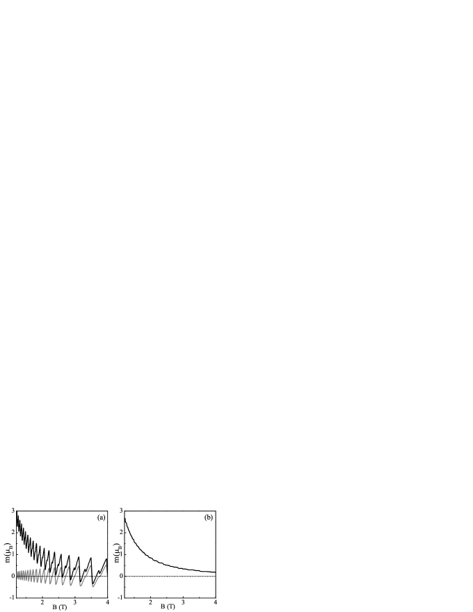
Figure 4: (a) Gray curve: The bulk contribution of the magnetization $m$ per hole (in units of $\mu_{B}$); Black curve: The total magnetization per hole $m$ (in units of $\mu_{B}$). (b) The edge contribution of the magnetization $m$ per hole (in units of $\mu_{B}$). In both figures, the Rashba SOC $\alpha=0$ and $L=600$nm. The other parameters are same as those in Fig. 2.

When the Rashba SOC is introduced, there is a energy competition between the Zeeman coupling and the Rashba SOC. Also, due to the entanglement between the orbital and spin degrees of freedom, it is difficult to distinguish their separate contributions to the total magnetization. These factors make the physical picture of the dHvA oscillations to change fundamentally, as shown in Fig. 5 for magnetization (per hole) $m$ as functions of $B$. One can see from these two figures that the Rashba SOC has no visible influence on the magnetic oscillations of the quantity $m$ at large values of $B$, where the Zeeman and spin-orbit coupling splitting are small compared to the Landau level splitting. At low magnetic field, however, the Rashba SOC modulation of the magnetic oscillations becomes obvious, which can be clearly seen by the enlarged plots of $\mu$ and $m$ in the inset in Fig. 5 for $B$ between $1.2$T and $1.4$T. For comparison, we also re-plot in Fig. 5 the cases without Rashba SOC. One can see from these two figures that the SOC brings about two new features at low magnetic field: (i) The sawtoothlike oscillating structure is inversed, i.e., the location of peaks in $\mu$ and $m$ with SOC correspond to the valleys without SOC. This inversion is due to the different Landau levels in the two cases. (ii) The oscillation mode is prominently modulated by SOC and a beating pattern appears. This beating behavior in the oscillations are due to the fact that the Landau levels are now unequally spaced due to the presence of SOC.

Figure 5: The dHvA oscillations of the magnetization (per hole) of 2D hole system as a function of external magnetic field $B$ with (dashed line, the Rashba SOC strength $\alpha=20\,$meV nm³) and without (solid line) Rashba SOC coupling at $T=0.2$K. Other parameters are same as those in Fig. 2. The inset is the enlarged magnetization oscillations between $1.2$T and $1.4$T.

Before ending this paper, let us briefly discuss the temperature effect. It is well known that the infinite temperature will blur the measured physical quantities, which including the dHvA oscillations of the magnetization. To illustrate the temperature effect, we plot in Fig.6 the magnetizations of the holes at different temperatures $T=0.5$, $1.0$, $2.0$, and $8.0\,$K, respectively. Obviously with the temperature increases, the amplitude decreases and the details of the oscillation tend to be blurred. At the temperature $T=8.0$K, the dHvA oscillations vanish and all the details are smeared out. However, the edge-state effect, which depends on the sample size and the external magnetic field, does not change with the temperature.

Figure 6: The dHvA oscillations of the magnetization (per hole) of 2D hole system as a function of the external magnetic field $B$ at different temperatures. The Rashba SOC strength is set as $\alpha=20\,$meV nm³. The other parameters are same as those in Fig. 2.

IV Summary

In conclusion, we have theoretically investigated the dHvA oscillations of the magnetization in the 2D heavy hole systems with boundaries in a perpendicular magnetic filed. Especially, we focus on the edge-state effect and the influence of the Rashba SOC on the magnetization. The results show that the effect of the edge states and Rashba SOC on the magnetization is less important when the magnitude of the magnetic field $B$ is so large. However, with $B$ decreasing, the effect becomes evident. First, the dHvA oscillation center of the magnetization will shift when the edge-state effect is considered. The contribution of the edge states to the total magnetization has a roughly linear relation with $1/B^{2}$ and $1/L$. When the Rashba SOC introduced, the sawtoothlike oscillating structure is inversed and a beating pattern appears. The phenomena caused by the Rashba SOC can be blurred when the temperature turns high. However, the edge-state effect do not change with the temperature changing.

ACKNOWLEDGMENTS

C. Fang and S. S. Li were supported by the National Basic Research Program of China (973 Program) grant No. G2009CB929300, and the National Natural Science Foundation of China under Grant Nos. 60821061 and 60776061. Z. G. Wang and P. Zhang were supported by the National Natural Science Foundation of China under Grant Nos. 10604010 and 60776063.

References

- Zhu et al. (2003) M. Zhu, A. Usher, A. J. Matthews, A. Potts, M. Elliott, W. G. Herrenden-Harker, D. A. Ritchie, and M. Y. Simmons, Phys. Rev. B 67, 155329 (2003).
- Schaapman et al. (2003) M. R. Schaapman, U. Zeitler, P. C. M. Christianen, J. C. Maan, D. Reuter, A. D. Wieck, D. Schuh, and M. Bichler, Phys. Rev. B 68, 193308 (2003).
- Gudmundsson et al. (2000) V. Gudmundsson, S. I. Erlingsson, and A. Manolescu, Phys. Rev. B 61, 4835 (2000).
- Niţá M et al. (2000) M. Niţá M, A. Aldea, and J. Zittartz, Phys. Rev. B 62, 15367 (2000).
- Harris et al. (2001) J. G. E. Harris, R. Knobel, K. D. Maranowski, A. C. Gossard, N. Samarth, and D. D. Awschalom, Phys. Rev. Lett. 86, 4644 (2001).
- Ohno (1998) H. Ohno, Science 281, 951 (1998).
- Wolf et al. (2001) S. A. Wolf, D. D. Awschalom, R. A. Buhrman, J. M. Daughton, S. von Molnar, M. L. Roukes, A. Y. Chtchelkanova, and D. M. Treger, Science 294, 1488 (2001).
- Gupta et al. (2001) J. A. Gupta, R. Knobel, N. Samarth, and D. D. Awschalom, Science 292, 2458 (2001).
- Peierls (1933) R. Peierls, Z. Phys. 81, 186 (1933).
- Vagner et al. (1983) I. D. Vagner, T. Maniv, and E. Ehrenfreund, Phys. Rev. Lett. 51, 1700 (1983).
- Shoenberg (1984) D. Shoenberg, J. Low Temp. Phys. 56, 417 (1984).
- L. Bremme and Ensslin (1999) T. I. L. Bremme and K. Ensslin, Phys. Rev. B 59, 7305 (1999).
- (13) Z. Wang, W. Zhang, and P. Zhang, e-print: arXiv: cond-mat/09021298.
- Schliemann and Loss (2005) J. Schliemann and D. Loss, Phys. Rev. B 71, 085308 (2005).
- Pala et al. (2004a) M. G. Pala, M. Governale, J. Konig, and U. Zulicke, Europhys. Lett. 65, 850 (2004a).
- Pala et al. (2004b) M. G. Pala, M. Governale, J. Konig, U. Zulicke, and G. Iannaccone, Phys. Rev. B 69, 045304 (2004b).
- Winkler (2000) R. Winkler, Phys. Rev. B 62, 4245 (2000).
- Winkler et al. (2002) R. Winkler, H. Noh, E. Tutuc, and M. Shayegan, Phys. Rev. B 65, 155303 (2002).
- Gerchikov and Subashiev (1992) L. Gerchikov and A. Subashiev, Sov. Phys. Semicond. 26, 73 (1992).
- Reynoso et al. (2004) A. Reynoso, G. Usaj, M. J. Sánchez, and C. A. Balseiro, Phys. Rev. B 70, 235344 (2004).
- Ma and Liu (2006) T. Ma and Q. Liu, Appl. Phys. Lett. 89, 112102 (2006).