Implementation of the quantum walk step operator in lateral quantum dots

Abstract

We propose a physical implementation of the step operator of the discrete quantum walk for an electron in a one-dimensional chain of quantum dots. The operating principle of the step operator is based on locally enhanced Zeeman splitting and the role of the quantum coin is played by the spin of the electron. We calculate the probability of successful transfer of the electron in the presence of decoherence due to quantum charge fluctuations, modeled as a bosonic bath. We then analyze two mechanisms for creating locally enhanced Zeeman splitting based on, respectively, locally applied electric and magnetic fields and slanting magnetic fields. Our results imply that a success probability of $>$ 90% is feasible under realistic experimental conditions.

The quantum walk (or quantum random walk) is the quantum-mechanical analogue of the classical random walk and describes the random walk behavior of a quantum particle. The concept ”quantum walk” was formally introduced by Aharonov et al. in 1993 ahar93 and suggested earlier by Feynman feyn65 . The essential difference with the classical random walk lies in the role of the coin: Whereas in the classical random walk the coin is a classical object with two possible measurement outcomes (”heads” or ”tails”), in the quantum walk the coin is a quantum-mechanical object - typically a two-level system such as a spin-1/2 particle - which can be measured along different bases and hence has a multi-sided character. As a result, the quantum walk exhibits strikingly different dynamic behavior compared to its classical counterpart due to interference between different possible paths. One example is faster propagation ahar93 : The root-mean-square distance from the origin $\langle x\rangle_{\rm rms}$ that is covered by a quantum walker grows linearly with the number of steps $N$ (thus corresponding to ballistic propagation), whereas for the classical random walk $\langle x\rangle_{\rm rms}\sim\sqrt{N}$ (corresponding to diffusive propagation). This property has been exploited to design new quantum computing algorithms kend06 . Both discrete and continuous time quantum walks have been extensively studied in recent years kemp03 , including investigations of decoherence brun03 and entanglement between quantum walkers vene05 .

As far as implementations of quantum walks in actual physical systems are concerned, several proposals have been put forward for a range of optical and atomic systems, such as optical cavities knig03 , cavity QED systems sand03 , trapped atoms and ions trav02 and linear optical elements path07 . On the experimental side, only a few realizations of quantum walks have been achieved: Discrete and continous quantum walks in NMR quantum systems du03 , discrete quantum walks using linear optical elements do05 and, most recently, a continuous quantum walk in an optical waveguide lattice pere07 .

For solid-state systems, no realizations of quantum walks exist so far. A recent proposal for implementation of a quantum algorithm using NAND operations in a tree of quantum dots relies on the continuous time quantum walk tayl07 .

In this paper we propose the first implementation of a discrete quantum walk in a solid-state quantum system, which consists of a single electron traveling in a one-dimensional chain of quantum dots. In particular, we focus on the implementation of the so-called step operator, the basic unit of the quantum walk. The step operator causes the electron to either move to the left or to the right depending on the state of the quantum coin, which in our model is represented by the spin of the electron. We calculate the spin-dependent transfer probability of the electron from one dot to the next in the presence of different energy level splittings in neighboring quantum dots (due to locally enhanced Zeeman splitting), taking into account the effects of decoherence due to gate voltage fluctuations dephasing . We then propose two physical mechanisms to achieve locally enhanced level splitting in a quantum dot using local electric and magnetic fields and find that under current experimental circumstances successful implementation of the step operator is possible with $>$ 90% probability.

Model of the step operator. - Consider a chain of three quantum dots in series, in which the middle dot (M) is occupied by a single electron, see Fig. 1.

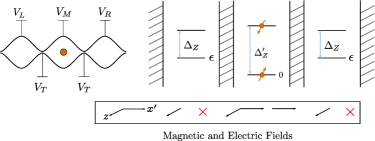
Figure 1: (left) A linear chain of 3 quantum dots in a magnetic field and (right) the corresponding energy level diagram. The direction of (locally) applied electric and magnetic fields in each dot is also indicated, a cross indicates no applied field. See the text for further explanation.

The energy level diagram shows the Zeeman splitting $\Delta_{z}^{(\prime)}$ of the lowest two levels in a magnetic field, and we assume that this splitting is larger in the middle dot by an amount $\Delta_{z}^{\prime}-\Delta_{z}$. The gate voltages $V_{L}$, $V_{M}$ and $V_{R}$ are used to shift the energy levels in the left, middle and right dot resp., and the gate voltages $V_{T}$ are used to tune the tunnel coupling between neighboring dots. The initial spin state of the electron is a superposition of spin-$\uparrow$ and spin-$\downarrow$ and our first goal is to design an implementation of the step operator such that it causes the electron to coherently move to the left (right) if it has spin-$\uparrow$ (spin-$\downarrow$) and to calculate the probability of succesful transfer for this process. To begin with, we assume the right dot to be decoupled from the other two and calculate the spin-dependent probabilities to find the electron in the left and middle dot at a given time. In the absence of decoherence - which is considered further below - the Hamiltonian for the spin-$\uparrow$ and spin-$\downarrow$ components of the electron is given by

$$H_{0,\sigma}=\left(\begin{array}[]{cc}A_{\sigma}&\lambda\\ \lambda&B_{\sigma}\end{array}\right),$$ (1)

in the basis $\{|L\rangle,|M\rangle\}$. Here ($A_{\uparrow}$,$B_{\uparrow}$) = ($\epsilon$,0), ($A_{\downarrow}$,$B_{\downarrow}$) = ($\epsilon+\Delta_{z}$,$\Delta_{z}^{{}^{\prime}}$) and $\lambda$ is the (spin-independent) tunnel coupling between the left and middle dot. The eigenvalues and -vectors of Eq. (1) are given by $E_{\pm,\sigma}=\frac{A_{\sigma}+B_{\sigma}}{2}\pm\frac{1}{2}\sqrt{(A_{\sigma}-B_{\sigma})^{2}+4\lambda^{2}}$, $|\psi_{+,\sigma}\rangle=(\sin\theta_{\sigma},\cos\theta_{\sigma})^{T}$ and $|\psi_{-,\sigma}\rangle=(\cos\theta_{\sigma},-\sin\theta_{\sigma})^{T}$, with $\tan\theta_{\sigma}\equiv\frac{\hbar\delta_{\sigma}+\sqrt{(\hbar\delta_{\sigma})^{2}+4\lambda^{2}}}{2\lambda}$, $\delta_{\uparrow}\equiv\epsilon/\hbar$ and $\delta_{\downarrow}=(\epsilon+\Delta_{z}-\Delta_{z}^{{}^{\prime}})/\hbar$. In the absence of decoherence, the solution of the density matrix equations $\dot{\rho}=-(i/\hbar)[H_{0,\sigma},\rho]$ for the population in the left dot is given by

$$\rho_{LL,\sigma}(t)=\frac{2\lambda^{2}}{(\hbar\omega_{\sigma})^{2}}\left[1-\cos(\omega_{\sigma}t)\right]$$ (2)

for initial conditions $\rho_{LL,\sigma}(0)=0$, $\rho_{MM,\sigma}(0)=1$ and $\hbar\omega_{\sigma}\equiv\sqrt{(\hbar\delta_{\sigma})^{2}+4\lambda^{2}}$. We see that the probability for the spin-$\uparrow$ component to be in the left dot and the spin-$\downarrow$ component to remain in the middle dot is 1 for $\frac{(\hbar\omega_{\uparrow})^{2}}{2\lambda^{2}}=1-\cos\left(2n\pi\frac{\omega_{\uparrow}}{\omega_{\downarrow}}\right)$, $n=0,1,2,\ldots$. The smallest $n$ that yields a solution to this equation for $\epsilon=0$ (zero detuning) is $n=1$, for which $\Delta_{z}-\Delta_{z}^{\prime}=2\sqrt{3}\,\lambda$ and $t=2\pi/\omega_{\downarrow}$. The second half of the step operator then consists of repeating the same procedure as described above for tunnel coupling between the middle and the right dot, now assuming the left dot to be decoupled.

Decoherence due to quantum fluctuations. - In reality, the time evolution of the occupation probabilities $\rho_{\sigma}$ is affected by decoherence due to coupling of the quantum dots to the environment. In typical experimental situations $k_{B}T<\hbar\omega_{\sigma}$, for $T\leq$ 100 mK and $\lambda\leq 1.5\,10^{-24}$ J pett05 ; kopp05 , so that quantum noise, rather than classical noise, is the dominant source of decoherence. Specifically, since the quantum walk step operator based on the Hamiltonian (1) involves tuning the tunnel couplings $\lambda$ - resulting in different charge occupations on neighboring dots - the probability distributions will be strongly affected by fluctuations of charge in the environment spinfluctuations . The quantum charge fluctuations we consider here are gate voltage fluctuations, which cause both fluctuations in the tunnel coupling $\lambda$ and in the energy levels $E_{\pm}$ of the Hamiltonian (1) romi07 . The Hamiltonian which describes the quantum dot system plus the environment is given by

$$H=H_{0}+V_{\epsilon}A_{\epsilon}+V_{\lambda}A_{\lambda}+H_{bath,\epsilon}+H_{bath,\lambda},$$ (3)

with $H_{0}$ the Hamiltonian (1) of the isolated system, $V_{\lambda}$ = $|L\rangle\langle M|+|M\rangle\langle L|$, $V_{\epsilon}$ = $|L\rangle\langle L|-|M\rangle\langle M|$, $A_{\epsilon(\lambda)}$ = $\sum_{k}c_{k,\epsilon(\lambda)}(b_{k,\epsilon(\lambda)}^{\dagger}+b_{k,\epsilon(\lambda)})$ and $H_{bath,\epsilon(\lambda)}$ = $\sum_{k}\hbar\omega_{k,\epsilon(\lambda)}b_{k,\epsilon(\lambda)}^{\dagger}b_{k,\epsilon(\lambda)}$. We model the environment as a bosonic bath weis99 with creation and annihilation operators $b_{k,\epsilon(\lambda)}^{\dagger}$ and $b_{k,\epsilon(\lambda)}$ and use the Born-Markov approximation cohe92 to calculate the time evolution of the spin-dependent occupation probabilities under the Hamiltonian (3), assuming weak coupling between the system and the environment and short correlation times of the boson baths (Markovian assumption). The baths are characterized by the symmetric and anti-symmetric spectral functions $S^{\pm}(\omega)$ with $S^{+}(\omega)=\coth\left(\frac{\hbar\omega}{2k_{B}T}\right)S^{-}(\omega)$ weis99 and we assume Ohmic baths with Lorentzian damping for which $S^{-}(\omega)=\alpha\hbar^{2}\omega\frac{1}{(\omega/\omega_{c})^{2}+1}$ with $\omega_{c}$ a cut-off frequency. The time evolution of the reduced density matrix $\rho_{ab}(t)$ is then given by $\frac{\mathrm{d}\rho_{ab}(t)}{\mathrm{d}t}=-i\omega_{ab}\rho_{ab}(t)+\sum_{cd}^{\textrm{(sec)}}R_{abcd}\rho_{cd}(t)$, with $\omega_{ab}\equiv(E_{a}-E_{b})/\hbar$ and $R_{abcd}$ the Bloch-Redfield tensor weis99 ; limitsum . Solving this master equation for the two-level system $\{|\psi_{+,\sigma}\rangle,|\psi_{-,\sigma}\rangle\}$ described above for an electron starting at $t=0$ in the middle dot yields for the evolution of the population $\rho_{--}$ of the groundstate $|\psi_{-}\rangle$ and the coherence terms $\rho_{-+}$:

$$\rho_{--,\sigma}(t) = \frac{1}{2}(\tanh(\frac{\hbar\omega_{\sigma}}{2k_{B}T})-\cos(2\theta_{\sigma}))e^{-\gamma_{1}t}+$$ (4a)

$$\frac{\coth(\frac{\hbar\omega_{\sigma}}{2k_{B}T})-1}{2\coth(\frac{\hbar\omega_{\sigma}}{2k_{B}T})}$$

$$\rho_{-+,\sigma}(t) = \rho_{+-,\sigma}^{*}(t)=-\sin\theta_{\sigma}\cos\theta_{\sigma}e^{-i\omega_{\sigma}t}e^{-\gamma_{2}t}$$ (4b)

with

$$\gamma_{1} = 4\pi^{2}\left(\alpha_{\lambda}\cos^{2}2\theta_{\sigma}+\alpha_{\epsilon}\sin^{2}2\theta_{\sigma}\right)\omega_{\sigma}\coth\left(\frac{\hbar\omega_{\sigma}}{2k_{B}T}\right)$$ (5a)

$$\gamma_{2} = \frac{\gamma_{1}}{2}+\frac{8\pi^{2}}{\hbar}\left(\alpha_{\lambda}\sin^{2}2\theta_{\sigma}+\alpha_{\epsilon}\cos^{2}2\theta_{\sigma}\right)k_{B}T.$$ (5b)

Eqns. (4) and (5) are valid in the limit $\gamma_{1}$, $\gamma_{2}$ $\ll|\hbar\omega_{\sigma}|,1/\bar{\tau}$ (with $\bar{\tau}$ the bath correlation time) cohe92 . The survival probability to remain in the middle dot at time $t$ is then given by

$$P_{M,\sigma}(t) = \frac{1}{2}\left[1+\cos(2\theta_{\sigma})\tanh\left(\frac{\hbar\omega_{\sigma}}{2k_{B}T}\right)(1-e^{-\gamma_{1}t})+\right.$$ (6)

$$\left.\cos^{2}(2\theta_{\sigma})\,e^{-\gamma_{1}t}+\sin^{2}(2\theta_{\sigma})\cos(\omega_{\sigma}t)\,e^{-\gamma_{2}t}\right]$$

and plotted for both spin-$\uparrow$ and spin-$\downarrow$ in Fig. 2.

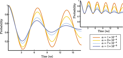
Figure 2: Survival probability [Eq. (6)] of the spin-$\uparrow$-component (main plot) and spin-$\downarrow$-component (inset) in the middle dot as a function of time $t$ for various values of $\alpha\equiv\alpha_{\lambda}=\alpha_{\epsilon}$ asta04 . Parameters used are $\hbar\delta_{\uparrow}=0$, $\hbar\delta_{\downarrow}=1\mu$eV, $\lambda=\left(2\sqrt{3}\right)^{-1}\,\mu$eV kopp05 , and $T=10$ mK.

Using typical experimental parameters (see figure caption and discussion below) we see that succesful transfer of the spin-$\uparrow$ component to the left dot while spin-$\downarrow$ remains in the middle dot occurs with probability $>$ 90% (for $\alpha\leq 3\cdot 10^{-4}$) at $t\approx 3.5$ ns.

Locally enhanced Zeeman splitting. - We now consider the question how a different Zeeman splitting in neighboring dots - as assumed in the calculations above - can be realized in practice. In particular, we propose two mechanisms to achieve locally enhanced Zeeman splitting. The first one is by application of a local transverse magnetic field and a local electric field and relies on spin-orbit interaction. Both tunable local magnetic and electric fields have recently been demonstrated experimentally kopp06 ; nowa07 . In our model, see Fig. 1, we assume that a local magnetic field (in addition to the global Zeeman-splitting field $\vec{B}$) and a local electric field $\vec{E}(t)$ are applied to the middle quantum dot. In the presence of spin-orbit interaction, the Hamiltonian for this middle dot is then given by $H=H_{0}+e\vec{E}(t)\cdot\vec{r}+\alpha\left(p_{x}\sigma_{y}-p_{y}\sigma_{x}\right)+\beta\left(-p_{x}\sigma_{x}+p_{y}\sigma_{y}\right)$, with $H_{0}$ the Hamiltonian given by Eq. (1), and $\alpha$ and $\beta$ resp. the Rashba and Dresselhaus spin-orbit coupling strengths. Using the Schrieffer-Wolff transformation, the Hamiltonian $H$ can be diagonalized to first order in the spin-orbit terms which yields, for the spin-dependent part, $H_{\rm eff}\equiv e^{S}He^{-S}=\frac{1}{2}g^{*}\mu_{B}\left(\vec{B}+\delta\vec{B}(t)\right)\cdot\vec{\sigma}$ borh06 . Here the effective magnetic field $\delta\vec{B}$ is given by $\delta\vec{B}=2\vec{B}\times\left(\vec{\Omega}_{1}(t)+\vec{n}\times\vec{\Omega}_{2}(t)\right)$, with $\vec{\Omega}_{1}(t)=\frac{e\hbar}{E_{Z}}\alpha_{1}\left(E_{y^{\prime}}/\lambda_{-},E_{x^{\prime}}/\lambda_{+},0\right)$, $\vec{\Omega}_{2}(t)=\frac{e\hbar}{E_{Z}}\beta_{1}\left(-E_{x^{\prime}}/\lambda_{-},E_{y^{\prime}}/\lambda_{+},0\right)$, $\alpha_{1}=\frac{\hbar}{m^{*}}\frac{E_{Z}\left(E_{Z}^{2}-(\hbar\omega_{0})^{2}\right)}{(E_{Z}^{2}-E_{1}^{2})(E_{Z}^{2}-E_{2}^{2})}$, $\beta_{1}=\frac{\hbar}{m^{*}}\frac{E_{Z}^{2}\hbar\omega_{c}}{(E_{Z}^{2}-E_{1}^{2})(E_{Z}^{2}-E_{2}^{2})}$, $\lambda_{\pm}=\hbar/(m^{*}(\beta\pm\alpha))$, $E_{Z}=g^{*}\mu_{B}B$, $E_{1,2}=\hbar(\sqrt{4\omega_{0}^{2}+\omega_{c}^{2}}\pm\omega_{c})/2$, with $\omega_{c}=eB/m^{*}$ the cyclotron frequency and $m^{*}\omega_{0}^{2}r^{2}/2$ the harmonic potential of the quantum dot hans07 . In these expressions we have used $x^{\prime}\equiv(x+y)/\sqrt{2}$ and $y^{\prime}\equiv(y-x)/\sqrt{2}$. Since for the step operator we require the eigenstates of the Hamiltonian $H$ to be $|\uparrow\rangle$ and $|\downarrow\rangle$ we must account for the fact that the eigenvectors of the effective Hamiltonian $H_{\rm eff}$ are transformed by $e^{S}$ with respect to the eigenvectors of $H$ corresponding to the same eigenvalues. We do this be requiring that the eigenvectors of $H_{\rm eff}$ are $e^{S}|\uparrow\rangle$ and $e^{S}|\downarrow\rangle$ to first order in the action $S$.

Let us assume the global magnetic field $\vec{B}$ to be parallel to the $\hat{z}$-axis. From the expression for $H_{\rm eff}$ it follows that in order to locally generate a different Zeeman splitting (along the $\hat{z}$-axis) in the middle dot compared to its neighboring dots, an additional tunable local magnetic field, e.g. along the $\hat{x}^{\prime}$-axis, and a tunable local electric field, also along the $\hat{x}^{\prime}$-axis, are required. We define the total (local) magnetic field $\vec{B}(t)=B_{0}\left(n_{x^{\prime}}(t),0,n_{z}\right)$. We use the expression for the effective magnetic field combined with the requirement for the eigenvectors of $H_{\textrm{eff}}$ to derive two implicit equations for the magnetic- and electric field in the $\hat{x}^{\prime}$-direction as a function of the local magnetic field $\delta B$ in the $\hat{z}$-direction:

$$n_{x^{\prime}}-n_{z}\frac{\gamma\alpha_{1}E_{x^{\prime}}}{\lambda_{+}}+n_{z}^{2}\frac{\gamma\beta_{1}E_{x^{\prime}}}{\lambda_{-}} = \left(1+\frac{\delta B}{B_{0}}\right)\frac{-2c}{1+c^{2}}$$ (7)

$$n_{z}+n_{x^{\prime}}\frac{\gamma\alpha_{1}E_{x^{\prime}}}{\lambda_{+}}-n_{x^{\prime}}n_{z}\frac{\gamma\beta_{1}E_{x^{\prime}}}{\lambda_{-}} = \left(1+\frac{\delta B}{B_{0}}\right)\frac{1-c^{2}}{1+c^{2}},$$ (8)

where we have defined $\gamma\equiv 2e\hbar/E_{Z}$ and $c\equiv\frac{eE_{x^{\prime}}}{m\omega_{0}^{2}}\left(\frac{1}{\lambda_{+}}+\frac{n_{z}\alpha_{2}}{\lambda_{-}}-(n_{x^{\prime}}^{2}+n_{z}^{2})\frac{\beta_{2}^{{}^{\prime}}}{\lambda_{+}}\right)\sigma_{y^{\prime}}$.

Fig. 3 shows the required fields $B_{x^{\prime}}$ and $E_{x^{\prime}}$ as a function of $B_{0}$ for typical experimental parameters and a local Zeeman splitting of $1$ $\mu eV$  parfields .

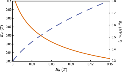
Figure 3: $E_{x^{\prime}}$ (solid line) and $B_{x^{\prime}}$ (dotted line) vs. $B_{0}$ for a local magnetic field $\delta B$ corresponding to a Zeeman splitting of $1$ $\mu eV$. Parameters used are $\hbar\omega_{0}=1$ meV hans07 , $m^{*}=0.067m_{e}$ (for GaAs hans07 ), $\lambda_{+}=2\,\mu$m, $\lambda_{-}=10\,\mu$m mill03 ; nowa07 , and $n_{z}=1$.

We see that in order to have an additional Zeeman splitting of 1 $\mu$eV (as assumed in Fig. 2), e.g. at $B_{0}$ = 0.05T magnetic and electric fields $B_{x^{\prime}}\sim 63$ mT and $E_{x^{\prime}}\sim 4.6\,10^{5}$ Vm^-1 are required. Although these values of $B_{x^{\prime}}$ and $E_{x^{\prime}}$ are (somewhat) larger than those that have been used so far in experiments lair07 ; nowa07 , they may well become available in the near future. Alternatively, one could use larger $B_{0}$ (corresponding to larger $B_{x^{\prime}}$ and smaller $E_{x^{\prime}}$) or smaller $\delta B_{z}$ (corresponding to smaller $B_{x^{\prime}}$ and $E_{x^{\prime}}$, but also smaller success probability). In addition, we note that in order to preserve the qubit’s quantum state, the fields need to be switched on and off adiabatically. The corresponding switching time $T$ of e.g. the tunable magnetic field then has to fulfill mess99 $T\gg\frac{\hbar n_{x^{\prime}}}{4n_{z}|g^{*}|\mu_{B}B_{0}}\sim 0.1$ ns. This timescale is well within experimental reach and compatible with the operation time (duration of electron transfer) $\approx 3.5$ ns that we estimated above.

Another method to generate different Zeeman fields in neighboring dots is by using a slanting magnetic field. The latter has recently been demonstrated for the first time by integrating a microsize ferromagnet in a double dot device pior08 . As a result of the slanting field, the orbital and spin degrees of freedom become hybridized, leading to an effective mixed charge-spin two-level system, where the role of the coin is played by the pseudospin instead of the real spin. A global magnetic field $\sim 2$ T magnetizes the ferromagnet and its inhomogeneity leads to a different Zeeman field in the two quantum dots of $\delta B_{z}\sim 10$ mT ($|\Delta_{z}-\Delta_{z}^{\prime}|\approx 4\cdot 10^{-26}$ J pior08 ). An advantage of this method compared to using spin-orbit interaction (as discussed above) is that no tunable magnetic fields but only tunable gate voltages are needed. A disadvantage is that the qubit is likely to be more sensitive to orbital decoherence.

Finally, we briefly discuss the question of how to extend our model from 3 quantum dots to a longer one-dimensional chain. In order for the electron to perform a quantum walk along the chain, opening and closing of tunnel barriers and aligning energy levels has to be applied at every position where the particle has a finite probability of being found. In addition, not only a step operator, but also a reinitialization operator $C$ of the coin (spin) degree of freedom is needed ahar93 . A common choice for $C$ is the Hadamard operator kemp03 , which can be implemented by two coherent rotations around different axes kopp06 ; nowa07 ; impl . The dynamics of a quantum walk of electrons along a one-dimensional chain of quantum dots in the presence of decoherence remains an interesting question for future research.

In conclusion, we have proposed an implementation of a discrete quantum walk step operator in a solid-state nanostructure consisting of a linear chain of 3 quantum dots. For currently available techniques to locally create enhanced Zeeman splitting and taking into account decoherence due to quantum charge fluctuations, we have analyzed the probability for coherent transfer of the electron to the left or right (conditioned on its spin), and predict that $>$ 90 % success probability is feasible. We hope that our results will stimulate a proof-of-principle experimental demonstration of the discrete quantum walk step operator in a solid-state nanosystem.

This work has been supported by the Netherlands Organisation for Scientific Research (NWO).

References

- (1) Y. Aharonov, L. Davidovich, and N. Zagury, Phys. Rev. A 48, 1687 (1993).
- (2) R.P. Feynman and A.R. Hibbs, Quantum mechanics and path integrals, (McGraw-Hill, New York, 1965).
- (3) V. Kendon, Phil. Trans. R. Soc. A 364, 3407 (2006).
- (4) Two recent reviews on quantum walks are J. Kempe, Contemp. Phys. 44, 307 (2003) and V. Kendon, Math. Struct. in Comp. Sci. 17, 1169 (2007).
- (5) T.A. Brun, H.A. Carteret, and A. Ambainis, Phys. Rev. Lett. 91, 130602 (2003); A. Romanelli et al., Physica A 347, 137 (2005); L. Ermann, J.P. Paz, and M. Saraceno, Phys. Rev. A 73, 012302 (2006); N.V. Prokof’ev and P.C.E. Stamp, ibid. 74, 020102 (2006); J. Kosik, V. Buzek, and M. Hillery, ibid., 022310 (2006); A.P. Hines and P.C.E. Stamp, Can. J Phys. 86, 541 (2008).
- (6) S.E. Venegas-Andraca et al., New J. Phys. 7, 221 (2005); G. Abal et al., Phys. Rev. A 73, 042302 (2006); Y. Omar et al., ibid. 74, 042304 (2006).
- (7) P.L. Knight, E. Roldan, and J.E. Sipe, Opt. Comm. 227, 147 (2003);
- (8) B.C. Sanders et al., Phys. Rev. A 67, 042305 (2003); G.S. Agarwal and P.K. Pathak, ibid. 72, 033815 (2005).
- (9) B.C. Travaglione and G.J. Milburn, Phys. Rev. A 65, 032310 (2002); W. Dür et al., ibid. 66, 052319 (2002); K. Eckert et al., ibid. 72, 012327 (2005); Z.-Y. Ma et al., ibid. 73, 013401 (2006).
- (10) P.K. Pathak and G.S. Agarwal, Phys. Rev. A 75, 032351 (2007).
- (11) J. Du et al., Phys. Rev. A 67, 042316 (2003); C.A. Ryan et al., ibid. 72, 062317 (2005).
- (12) B. Do et al., J. Opt. Soc. Am. B 22, 499 (2005); P. Zhang et al., Phys. Rev. A 75, 052310 (2007).
- (13) H.B. Perets et al., Phys. Rev. Lett. 100, 170506 (2008).
- (14) J.M. Taylor, arXiv:0708.1484v1 [quant-ph]
- (15) In Ref. tayl07 the effects of dephasing are taken into account in a phenomenological way and modeled by a dephasing rate .
- (16) See e.g. J.R. Petta et al., Science 309, 2180 (2005).
- (17) F.H.L. Koppens et al, Science 309, 1346 (2005).
- (18) Fluctuations in the nuclear spin environment, which is coupled to the electron spin via the hyperfine interaction, are slow (typically of the order of microseconds or more, see e.g. J.M. Taylor et al., Phys. Rev. B 76, 035315 (2007)). The nuclear field therefore acts as a frozen external field during the step operation and we neglect its fluctuations in our model.
- (19) A. Romito and Y. Gefen, Phys. Rev. B 76, 195318 (2007).
- (20) U. Weiss, Quantum dissipative systems, (World Scientific, Singapore, 1999).
- (21) C. Cohen-Tannoudji, J. Dupont-Roc, and G. Grynberg, Atom-photon interactions, (Wiley, New York, 1998).
- (22) The sum extends over terms with (secular constraint) where is the timescale of the Markovian course-grained evolution cohe92 .
- (23) Values of in this range were measured by O. Astafiev et al., Phys. Rev. Lett. 93, 267007 (2004).
- (24) K.C. Nowack et al., Science 318, 1430 (2007).
- (25) F.H.L. Koppens et al., Nature 442, 766 (2006).
- (26) M. Borhani, V. N. Golovach, and D. Loss, Phys. Rev. B 73, 155311 (2006); V. N. Golovach, M. Borhani, and D. Loss, ibid. 74, 165319 (2006).
- (27) For a recent review on spin qubits in quantum dots see R. Hanson et al., Rev. Mod. Phys. 79, 1217 (2007).
- (28) Similar values for and are found for an in-plane global magnetic field and out-of-plane local fields.
- (29) J.B. Miller et al., Phys. Rev. Lett. 90, 076807 (2003); S. Amasha et al., ibid. 100, 046803 (2008).
- (30) E.A. Laird et al., Phys. Rev. Lett. 99, 246601 (2007).
- (31) A. Messiah, Quantum Mechanics, (Dover, 1999), Ch. XVII.
- (32) M. Pioro-Ladrière et al., Nature physics 4, 776 (2008); Y. Tokura et al., Phys. Rev. Lett. 96, 047202 (2006).
- (33) M. Nielsen and I. Chuang, Quantum Computation and Quantum Information, (Cambridge University Press, Cambridge, 2000).