Phase diagram of the Heisenberg antiferromagnet with four-spin interactions

Abstract

We study the quantum phase diagram of the Heisenberg planar antiferromagnet with a subset of four-spin ring exchange interactions, using the recently proposed heirarchical mean-field approach. By identifying relevant degrees of freedom, we are able to use a single variational anzatz to map the entire phase diagram of the model and uncover the nature of its various phases. It is shown that there exists a transition between a Néel state and a quantum paramagnetic phase, characterized by broken translational invariance. The non-magnetic phase preserves the lattice rotational symmetry, and has a correlated plaquette nature. Our results also suggest that this phase transition can be properly described within the Landau paradigm.

I Introduction

Quantum phases of matter and their transitions are of fundamental concern to modern condensed matter physics Sachdev_1999 . Such interest is motivated not only by potential technical applications, but also on purely scientific grounds. Research in this field may lead to a deeper understanding of the fundamental working principles behind Nature’s behavior, and often original new physical theories emerge. One of them, recently proposed in Ref. Sachdev_2004, , predicts the existence of a class of systems whose critical behavior lies outside the scope of the Landau theory of phase transitions Landau_1999 . Critical points in these systems are characterized by the deconfinement of fractionalized excitations, parameterizing the original degrees of freedom, which occurs right at the transition. It was observed that this scenario can, in principle, be realized in spin systems, which exhibit a second-order phase transition point characterized by the simultaneous breakdown of a continuous (e.g. spin $SU(2)$) and a discrete (e.g. lattice) symmetries, in such a way that symmetry groups on opposite sides of the transition are not group-subgroup related. Such critical points cannot be described in the framework of Landau’s theory.

According to Ref. Sachdev_2004, , there should exist a substantial number of spin systems, which exhibit deconfined critical points. For instance, frustrated two-dimensional (2D) antiferromagnets (AFs), like the $J_{1}$-$J_{2}$ model, are believed to fall into this category. However, there seems to be no experimental or theoretical proof of this claim. Another class of models believed to display such a behavior includes non-frustrated AFs with multi-spin exchange interactions. One such model was studied by Sandvik Sandvik_2007 and other authors Melko_2008_prl ; Melko_2008_prb and, although seemingly artificial, it provides a playground for testing new theories. Their Quantum Monte Carlo (QMC) simulations claimed numerical evidence for the deconfined quantum criticality scenario.

The model studied in Ref. Sandvik_2007, is a Heisenberg AF with a subset of four-spin ring exchange interactions, defined on a square lattice (named the $J$-$Q$ model)

$$H=J\sum_{\langle{\bm{i}}{\bm{j}}\rangle}{\bm{S}}_{\bm{i}}{\bm{S}}_{\bm{j}}-Q\sum_{\langle{\bm{i}}{\bm{j}}{\bm{k}}{\bm{l}}\rangle}\biggl{(}{\bm{S}}_{\bm{i}}{\bm{S}}_{\bm{j}}-\frac{1}{4}\biggr{)}\biggl{(}{\bm{S}}_{\bm{k}}{\bm{S}}_{\bm{l}}-\frac{1}{4}\biggr{)},$$

where $Q\geqslant 0$, ${\bm{i}},{\bm{j}},\ldots$ denote sites in a 2D square lattice and ${\bm{S}}_{\bm{i}}$ are spin-$1/2$ operators. The first summation extends over bonds (nearest neighbor sites). The second term contains two sums over plaquettes (sites of the dual lattice): first, $({\bm{i}}{\bm{j}})$ and $({\bm{k}}{\bm{l}})$ denote parallel horizontal links of the plaquette, and then $({\bm{i}}{\bm{k}})$ and $({\bm{j}}{\bm{l}})$ correspond to parallel vertical bonds. It was concluded Sandvik_2007 that there exists a critical point at $Q_{c}/J\sim 25$ separating the antiferromagnetic phase from a valence-bond solid (VBS) state, whose nature is, strictly speaking, unclear Sandvik_2007 but the calculations suggested a columnar (dimer) order in this paramagnetic region.

In the present paper we study the phase diagram of the $J$-$Q$ model, using a recently proposed hierarchical mean-field (HMF) technique Isaev_2009 ; Ortiz_2003 . The main idea of the method revolves around the concept of a relevant degree of freedom (a “quark”) – spin cluster in this particular case – which can be used to build up the system. The initial Hamiltonian is then rewritten in terms of these coarse-grained variables and a mean-field approximation is applied to determine properties of the system. Thus, the (generally) exponentially hard problem of determining the ground state of the system is reduced to a polynomially complex one. At the same time, essential quantum correlations, which drive the physics of the problem, are captured by the local representation. In other words, provided the quark is chosen properly, even a simple single mean-field approximation, performed on these degrees of freedom, will yield the correct phase diagram. Moreover, our HMF ansatz provides an educated nodal surface that can, in principle, be used in conjunction with fixed-node (or constrained path Carlson_1999 ) QMC approaches to further improve correlations, and thus energy estimates, in those cases when there is a sign (phase) problem.

It is important to emphasize the simplicity of our method. In this work we concentrate on symmetries of the various phases, exhibited by the $J$-$Q$ model. By using a more sophisticated variational ansatz (e.g. a Jastrow–type correlated wavefunction), one can also improve numerical values of the observable quantities and phase transition points, but the physical picture will remain intact. Nevertheless, the HMF method was quite accurate to yield the quantitatively correct phase diagram Isaev_2009 of the $J_{1}$-$J_{2}$ model, whose behavior is driven by the interplay of two gapless phases: the Néel and columnar AF states. In the $J$-$Q$ model the large-$Q$ phase is gapped. Due to its real-space nature, the HMF method should be appropriate for this model. Indeed, our recent studies SS_2009 of another gapped system – the Heisenberg model on the Shastry-Sutherland lattice – support this assumption.

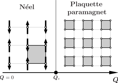
Figure 1: Schematic phase diagram of the $J$-$Q$ model, obtained in the present paper. The translationally invariant AF phase with broken $SU(2)$ symmetry and the singlet paramagnetic state are separated by a quantum phase transition at $Q=Q_{c}$. Results of our calculations indicate that this transition is continuous, but we can not rigorously discard the possibility that it becomes weakly first order in the thermodynamic limit. The non-magnetic phase breaks the lattice translational symmetry and is a plaquette paramagnet.

Our findings are summarized in Fig. 1. There indeed exists a non-magnetic phase, which we found to be of a correlated plaquette type, and not of a dimer character, separated from the Néel state by a second-order phase transition. However, the numerical value of the critical point, $Q_{c}/J\sim 2$, which we obtained, is quite different from that of Ref. Sandvik_2007, . Our results are consistent with data obtained from exact diagonalization of finite spin clusters which, given the fact that the system is gapped in the paramagnetic phase for $Q\geqslant Q_{c}$, should be reliable in this region. Although we found the phase transition to be of the Landau second-order type, due to the real-space nature of the method (which explicitly breaks the lattice translational invariance), we cannot rigorously rule out the possibility that this phase transition becomes weakly first order as one scales the degree of freedom towards the thermodynamic limit.

In the next section we set up the formalism. The results are presented in Sec. III, followed by a discussion in Sec. IV.

II Coarse graining and HMF approximation

For our purposes it is convenient to separate the two and four spin terms in the $J$-$Q$ Hamiltonian:

$$H= -\frac{2NQ}{16}+\biggl{(}J+\frac{Q}{2}\biggr{)}\sum_{\langle{\bm{i}}{\bm{j}}\rangle}{\bm{S}}_{\bm{i}}{\bm{S}}_{\bm{j}}-$$

$$-Q\sum_{\langle{\bm{i}}{\bm{j}}{\bm{k}}{\bm{l}}\rangle}({\bm{S}}_{\bm{i}}{\bm{S}}_{\bm{j}})({\bm{S}}_{\bm{k}}{\bm{S}}_{\bm{l}}).$$ (1)

A satisfactory coarse graining procedure should partition the lattice into spin clusters (quarks), containing $N_{q}$ sites, that explicitly preserve symmetries of the Hamiltonian. In particular, the $J$-$Q$ Hamiltonian is explicitly spin–$SU(2)$ invariant. Moreover, it is invariant under transformations from the lattice rotational group $C_{4}$. Therefore, we will consider only symmetry preserving degrees of freedom: (i) plaquettes ($2\times 2$ spin clusters) and (ii) $4\times 4$ spin clusters. Each cluster state will be associated with a hard-core bosonic operator $\gamma$. These operators are Schwinger bosons of $SU\bigl{(}2^{N_{q}}\bigr{)}$ and must obey the local constraint: $\sum_{a}\gamma^{\dagger}_{ia}\gamma_{ia}=1$. They define the hierarchical language Ortiz_2003 for our problem.

From the form of Eq. (1) it is clear Isaev_2009 that the (equivalent and exact) bosonic Hamiltonian will contain not only two-body scattering processes, but also four-boson interactions. Therefore, we can write down symbolically:

$$H= \sum_{i}\bigl{(}H_{\Box}\bigr{)}_{a^{\prime}a}\gamma^{\dagger}_{ia^{\prime}}\gamma_{ia}+$$

$$+\sum_{\langle ij\rangle}\bigl{(}H^{2}_{\rm int}\bigr{)}^{a^{\prime}_{1}a^{\prime}_{2}}_{a_{1}a_{2}}\gamma^{\dagger}_{ia_{1}^{\prime}}\gamma^{\dagger}_{ja_{2}^{\prime}}\gamma_{ia_{1}}\gamma_{ja_{2}}+$$

$$+ \sum_{\langle i_{1}i_{2}i_{3}i_{4}\rangle_{h}}\bigl{(}H^{4h}_{\rm int}\bigr{)}^{a^{\prime}_{1}a^{\prime}_{2};a^{\prime}_{3}a^{\prime}_{4}}_{a_{1}a_{2};a_{3}a_{4}}\prod_{\mu=1}^{4}\gamma^{\dagger}_{i_{\mu}a_{\mu}^{\prime}}\gamma_{i_{\mu}a_{\mu}}+$$

$$+ \sum_{\langle i_{1}i_{2}i_{3}i_{4}\rangle_{v}}\bigl{(}H^{4v}_{\rm int}\bigr{)}^{a^{\prime}_{1}a^{\prime}_{3};a^{\prime}_{2}a^{\prime}_{4}}_{a_{1}a_{3};a_{2}a_{4}}\prod_{\mu=1}^{4}\gamma^{\dagger}_{i_{\mu}a_{\mu}^{\prime}}\gamma_{i_{\mu}a_{\mu}},$$ (2)

where $a,\ldots$ label states in the Hilbert space of a quark, $i,j,\ldots$ denote sites in the coarse grained lattice, and summations are assumed over all repeated indices. The term with $H^{2}_{\rm int}$ encodes two-body interactions, while the last two lines describe the correlated four-boson scattering. The superscript $h$ indicates that $i_{1}i_{2}$ and $i_{3}i_{4}$ are horizontal links of a plaquette, and similarly $v$ denotes the case when $i_{1}i_{3}$ and $i_{2}i_{4}$ are vertical links of the same plaquette.

We will investigate the phase diagram of the $J$-$Q$ model using the HMF approximation whose variational state assumes that the hard-core bosons form an insulating state. Further, we introduce a new set of bosonic operators, related to the old ones by a real site-independent canonical transformation:

$$\gamma_{ia}=R_{a}^{n}\Gamma_{in};\,\,\,R_{a}^{n}R_{b}^{n}=\delta_{ab},\,\,\,R_{a}^{n}R_{a}^{m}=\delta_{nm}$$

and write the variational ground state in the form:

$$|\psi_{0}\rangle=\prod_{i}\Gamma^{\dagger}_{i0}|0\rangle,$$ (3)

where $n=0$ denotes the lowest energy single-particle mode (we shall also denote: $R_{a}^{0}\equiv R_{a}$), and $|0\rangle$ represents the vacuum. It is important to emphasize that although the coarse graining procedure preserves the symmetries of the Hamiltonian, some of them can be spontaneously broken at the mean-field level as a result of self-consistency. In particular, the columnar dimer state is contained in the wavefunction (3) although, as we will see below, it never appears as a stable solution.

We have explicitly separated the four-boson interaction in the Hamiltonian (2) into horizontal and vertical link contributions. This distinction is important because these two terms must be properly symmetrized to fulfill bosonic statistics. In particular, the term $H^{4h}_{\rm int}$ has to be symmetrized only with respect to indices in the same group, and groups as a whole (groups are separated by semicolons), i.e. one needs to take into account only the following permutations: $(1\leftrightarrow 2)$, $(3\leftrightarrow 4)$ and simultaneously ($1\leftrightarrow 3$, $2\leftrightarrow 4$). Analogously, in the term $H^{4v}_{\rm int}$ only the permutations $(1\leftrightarrow 3)$, $(2\leftrightarrow 4)$ and ($1\leftrightarrow 2$, $3\leftrightarrow 4$) should be accounted for.

The problem then reduces to minimization of the energy functional:

$$\frac{N_{q}E_{0}[R]}{N}= (H_{\Box})_{a^{\prime}a}R_{a^{\prime}}R_{a}+$$

$$+\bigl{(}H^{2}_{\rm int}\bigr{)}^{a^{\prime}_{1}a^{\prime}_{2}}_{a_{1}a_{2}}\prod_{\nu=1}^{2}R_{a_{\nu}^{\prime}}R_{a_{\nu}}+$$ (4)

$$+\bigl{(}H^{4h}_{\rm int}+H^{4v}_{\rm int}\bigr{)}^{a^{\prime}_{1}a^{\prime}_{2};a^{\prime}_{3}a^{\prime}_{4}}_{a_{1}a_{2};a_{3}a_{4}}\prod_{\nu=1}^{4}R_{a_{\nu}^{\prime}}R_{a_{\nu}}$$

under the constraint $R_{a}R_{a}=1$, which leads to the self-consistent eigenvalue equation:

$$\bigl{(}H_{HF}\bigr{)}_{ab}R_{b}=\mu R_{a}$$ (5a)

with the chemical potential $$\mu$$ being the lowest eigenvalue of the Hartree-Fock Hamiltonian:

$$\bigl{(}H_{HF}\bigr{)}_{ab}= \bigl{(}H_{\Box}\bigr{)}_{ab}+2\bigl{(}H_{\rm int}^{2}\bigr{)}_{a_{1}a}^{a^{\prime}_{1}b}R_{a^{\prime}_{1}}R_{a_{1}}+$$

$$+4\bigl{(}H^{4h}_{\rm int}+H^{4v}_{\rm int}\bigr{)}_{a_{1}a_{2}a_{3}a}^{a^{\prime}_{1}a^{\prime}_{2}a^{\prime}_{3}b}\prod_{\mu=1}^{3}R_{a^{\prime}_{\mu}}R_{a_{\mu}}.$$ (5b)

Once the amplitude $R_{a}$ is determined, the ground state energy (GSE) can be computed using Eq. (4).

Although we have formulated the HMF method for spin-$1/2$ systems, it can be straightforwardly extended to higher spins as well.

Besides the GSE we will also be interested in computing the staggered magnetization $M_{z}$, and the two-component VBS “order parameter” Sachdev_2008 :

$${\rm Re}\Psi= \frac{1}{N}\sum_{\bm{x}}(-1)^{x}{\bm{S}}_{{\bm{x}}+{\bm{e}}_{x}}{\bm{S}}_{\bm{x}};$$

$${\rm Im}\Psi= \frac{1}{N}\sum_{\bm{x}}(-1)^{y}{\bm{S}}_{{\bm{x}}+{\bm{e}}_{y}}{\bm{S}}_{\bm{x}},$$

which allows us to characterize lattice point group symmetries of a state.

In the rest of this section we will sketch the HMF calculation of $E_{0}$, $M_{z}$ and $\Psi$ for the case of plaquettes, and only present final expressions for the $4\times 4$ clusters. The interested reader is referred to Ref. Isaev_2009, , where the technique is analyzed and developed in greater detail. For simplicity we shall put $J\equiv 1$.

Figure 2: The plaquette lattice. Thick lines denote interactions $J+Q/2$. The circles indicate four-spin terms of strength $Q$ in the Hamiltonian (1). Small-sized numbers label spins within a plaquette, while the larger ones label plaquettes.

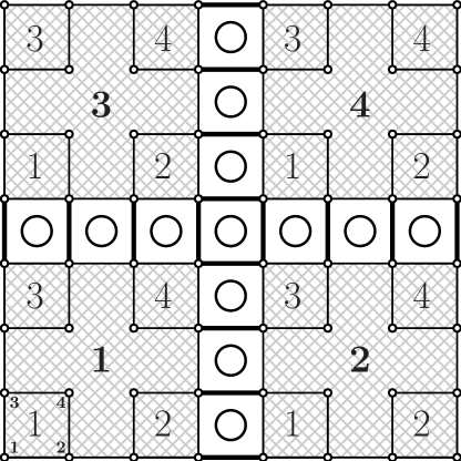
Figure 3: Connectivity of the lattice formed by $4\times 4$ spin clusters. Small circles indicate spins.Bold numbers label the $4\times 4$ clusters, while thin ones denote plaquettes. Other notations, are the same as in Fig. 2.

(i) The plaquette degree of freedom

We start by considering the simplest way to cover the lattice – with plaquettes, as shown in Fig. 2. At the same time we introduce notations and concepts, which will be used in the following subsection.

The Hamiltonian for an isolated plaquette has the form:

$$H_{\Box}= \biggl{(}1+\frac{Q}{2}\biggr{)}({\bm{S}}_{1}+{\bm{S}}_{4})({\bm{S}}_{2}+{\bm{S}}_{3})-$$

$$-Q\bigl{[}({\bm{S}}_{1}{\bm{S}}_{2})({\bm{S}}_{3}{\bm{S}}_{4})+({\bm{S}}_{1}{\bm{S}}_{3})({\bm{S}}_{2}{\bm{S}}_{4})\bigr{]}.$$ (6)

The interaction of this plaquette with the rest of the system can be conveniently partitioned according to (2) as:

$$H_{\rm int}=H^{2}_{\rm int}+H^{4h}_{\rm int}+H^{4v}_{\rm int},$$

where appropriately symmetrized individual terms are given by:

$$H^{2}_{\rm int}=\frac{1+Q/2}{2}\bigl{[} ({\bm{S}}_{11}+{\bm{S}}_{14})({\bm{S}}_{22}+{\bm{S}}_{23})+$$

$$+({\bm{S}}_{12}+{\bm{S}}_{13})({\bm{S}}_{21}+{\bm{S}}_{24})\bigr{]}-$$ (7a)

$$-\frac{Q}{2}\bigl{[}({\bm{S}}_{11} {\bm{S}}_{12})({\bm{S}}_{23}{\bm{S}}_{24})+({\bm{S}}_{11}{\bm{S}}_{23})({\bm{S}}_{12}{\bm{S}}_{24})+$$

$$+({\bm{S}}_{12} {\bm{S}}_{14})({\bm{S}}_{21}{\bm{S}}_{23})+({\bm{S}}_{12}{\bm{S}}_{21})({\bm{S}}_{14}{\bm{S}}_{23})+$$

$$+({\bm{S}}_{13} {\bm{S}}_{14})({\bm{S}}_{21}{\bm{S}}_{22})+({\bm{S}}_{13}{\bm{S}}_{21})({\bm{S}}_{14}{\bm{S}}_{22})+$$

$$+({\bm{S}}_{11} {\bm{S}}_{22})({\bm{S}}_{13}{\bm{S}}_{24})+({\bm{S}}_{11}{\bm{S}}_{13})({\bm{S}}_{22}{\bm{S}}_{24})\bigr{]};$$

$$H^{4h}_{\rm int}=-\frac{Q}{8} \bigl{[}({\bm{S}}_{14}{\bm{S}}_{23}+{\bm{S}}_{24}{\bm{S}}_{13})({\bm{S}}_{32}{\bm{S}}_{41}+{\bm{S}}_{31}{\bm{S}}_{42})+$$

$$+({\bm{S}}_{34} {\bm{S}}_{43}+{\bm{S}}_{44}{\bm{S}}_{33})({\bm{S}}_{12}{\bm{S}}_{21}+{\bm{S}}_{11}{\bm{S}}_{22})\bigr{]};$$ (7b)

$$H^{4v}_{\rm int}=-\frac{Q}{8} \bigl{[}({\bm{S}}_{14}{\bm{S}}_{32}+{\bm{S}}_{12}{\bm{S}}_{34})({\bm{S}}_{23}{\bm{S}}_{41}+{\bm{S}}_{21}{\bm{S}}_{43})+$$

$$+({\bm{S}}_{24} {\bm{S}}_{42}+{\bm{S}}_{22}{\bm{S}}_{44})({\bm{S}}_{13}{\bm{S}}_{31}+{\bm{S}}_{11}{\bm{S}}_{33})\bigr{]}.$$ (7c)

It is convenient to work in the basis which diagonalizes the $Q$-independent part of $H_{\Box}$, Eq. (6). Such is, for instance, the basis of eigenstates of the total angular momentum of the plaquette:

$$| a\rangle=|l_{1}l_{2}LM\rangle,$$ (8)

$${\bm{l}}_{1}={\bm{S}}_{1}+{\bm{S}}_{4};\,\,\,{\bm{l}}_{2}={\bm{S}}_{2}+{\bm{S}}_{3};\,\,\,{\bm{L}}={\bm{l}}_{1}+{\bm{l}}_{2}.$$

The matrix elements, which appear in Eq. (4)

$$\bigl{(}H^{2}_{\rm int}\bigr{)}^{a^{\prime}_{1}a^{\prime}_{2}}_{a_{1}a_{2}}\equiv \langle a^{\prime}_{1}a^{\prime}_{2}|H^{2}_{\rm int}|a_{1}a_{2}\rangle;$$

$$\bigl{(}H^{4h,v}_{\rm int}\bigr{)}^{a^{\prime}_{1}a^{\prime}_{2};a^{\prime}_{3}a^{\prime}_{4}}_{a_{1}a_{2};a_{3}a_{4}} \equiv\langle a^{\prime}_{1}a^{\prime}_{2};a^{\prime}_{3}a^{\prime}_{4}|H^{4h,v}_{\rm int}|a_{1}a_{2};a_{3}a_{4}\rangle$$

can now be computed using the angular momentum addition theorems.

The staggered magnetization (along the $z$-axis) within a plaquette is given by

$$M_{z}=\frac{1}{4}\bigl{(}S^{z}_{1}+S^{z}_{4}-S^{z}_{2}-S^{z}_{3}\bigr{)}_{ab}R_{a}R_{b},$$ (9)

while the function $\Psi$ can be written in the plaquette representation as:

$${\rm Re}\Psi= \frac{1}{N}\sum_{i}\bigl{[}{\bm{S}}_{i1}{\bm{S}}_{i2}+{\bm{S}}_{i3}{\bm{S}}_{i4}\bigr{]}-$$

$$-\frac{1}{N}\sum_{i}\bigl{[}{\bm{S}}_{i2}{\bm{S}}_{i+\hat{x},1}+{\bm{S}}_{i4}{\bm{S}}_{i+\hat{x},3}\bigr{]};$$ (10)

$${\rm Im}\Psi= \frac{1}{N}\sum_{i}\bigl{[}{\bm{S}}_{i1}{\bm{S}}_{i3}+{\bm{S}}_{i2}{\bm{S}}_{i4}\bigr{]}-$$

$$-\frac{1}{N}\sum_{i}\bigl{[}{\bm{S}}_{i3}{\bm{S}}_{i+\hat{y},1}+{\bm{S}}_{i4}{\bm{S}}_{i+\hat{y},2}\bigr{]}.$$

In these equations the indices $i$ and $\hat{x}$ denote sites and basis vectors of the plaquette lattice.

Figure 4: Ground state energy as a function of $Q/J$ for plaquettes [case (i)] and $4\times 4$ spin clusters [case (ii)].

(ii) $4\times 4$ spin clusters

The coarse grained lattice obtained by choosing the $4\times 4$ cluster as a degree of freedom is shown in Fig. 3. Each spin operator carries three indices: label of a cluster, label of a plaquette within this cluster, and the position within this plaquette. Writing down the cluster self-energy and the inter-cluster interactions is a straightforward, but tedious task, which can be accomplished along the lines presented in the previous subsection. Therefore, here we give only final expressions for $M_{z}$ and $\Psi$.

The staggered magnetization of a cluster is given by an equation analogous to (9):

$$M_{z}=\sum_{i=1}^{4}\bigl{(}S^{z}_{i1}+S^{z}_{i4}-S^{z}_{i2}-S^{z}_{i3}\bigr{)}_{A^{\prime}A}R_{A^{\prime}}R_{A},$$ (11)

where the summation extends over plaquettes within a cluster, and we used capital indices $A$ to label states of the cluster. The function $\Psi$ can be written as

$${\rm Re}\Psi=\frac{1}{N}\sum_{i} \bigl{(}{\bm{S}}_{i11}{\bm{S}}_{i12}+{\bm{S}}_{i13}{\bm{S}}_{i14}+{\bm{S}}_{i31}{\bm{S}}_{i32}+$$

$$+{\bm{S}}_{i33}{\bm{S}}_{i34}+{\bm{S}}_{i21}{\bm{S}}_{i22}+{\bm{S}}_{i23}{\bm{S}}_{i24}+$$

$$+{\bm{S}}_{i41}{\bm{S}}_{i42}+{\bm{S}}_{i43}{\bm{S}}_{i44}-{\bm{S}}_{i12}{\bm{S}}_{i21}-$$

$$-{\bm{S}}_{i14}{\bm{S}}_{i23}-{\bm{S}}_{i32}{\bm{S}}_{i41}-{\bm{S}}_{i34}{\bm{S}}_{i43}\bigr{)}-$$

$$-\frac{1}{N}\sum_{i} \bigl{[}{\bm{S}}_{i22}{\bm{S}}_{i+\hat{x},11}+{\bm{S}}_{i24}{\bm{S}}_{i+\hat{x},13}+$$

$$+{\bm{S}}_{i42}{\bm{S}}_{i+\hat{x},31}+{\bm{S}}_{i44}{\bm{S}}_{i+\hat{x},33}\bigr{]};$$ (12)

$${\rm Im}\Psi=\frac{1}{N}\sum_{i} \bigl{(}{\bm{S}}_{i11}{\bm{S}}_{i13}+{\bm{S}}_{i12}{\bm{S}}_{i14}+{\bm{S}}_{i21}{\bm{S}}_{i23}+$$

$$+{\bm{S}}_{i22}{\bm{S}}_{i24}+{\bm{S}}_{i31}{\bm{S}}_{i33}+{\bm{S}}_{i32}{\bm{S}}_{i34}+$$

$$+{\bm{S}}_{i41}{\bm{S}}_{i43}+{\bm{S}}_{i42}{\bm{S}}_{i44}-{\bm{S}}_{i13}{\bm{S}}_{i31}-$$

$$-{\bm{S}}_{i14}{\bm{S}}_{i32}-{\bm{S}}_{i23}{\bm{S}}_{i41}-{\bm{S}}_{i24}{\bm{S}}_{i42}\bigr{)}-$$

$$-\frac{1}{N}\sum_{i} \bigl{[}{\bm{S}}_{i33}{\bm{S}}_{i+\hat{y},11}+{\bm{S}}_{i34}{\bm{S}}_{i+\hat{y},12}+$$

$$+{\bm{S}}_{i43}{\bm{S}}_{i+\hat{y},21}+{\bm{S}}_{i44}{\bm{S}}_{i+\hat{y},22}\bigr{]}.$$

III Results

Figure 5: Second-order derivative $d^{2}E_{0}/NdQ^{2}$ (main panel) as a function of $Q/J$ for cases (i) and (ii). The discontinuity at $Q/J\sim 1.61$ ($2\times 2$) and $Q/J\sim 2.0$ ($4\times 4$) indicates a second-order phase transition point. The inset shows the extrapolation of the jump $g=Jd^{2}E_{0}/NdQ^{2}|_{Q_{c}-0}^{Q_{c}+0}$ to $N_{q}\to\infty$.

Figure 6: Staggered magnetization (main panel), Eqs. (9) and (11), as a function of $Q/J$ for cases (i) and (ii). The values of $Q_{c}$ are: $Q_{c}/J=1.61$ for case (i) and $Q_{c}/J=2.00$ for case (ii). The inset shows the scaling of $Q_{c}$.

We can now proceed with solution of the mean-field equation (5), supplemented by Eqs. (6), (7) for the case (i) and analogous expressions in the case (ii).

The physical quantities that we want to compute in the first place are the GSE and the staggered magnetization. These are given by Eq. (4) and Eqs. (9) for the case (i), and (11) for the case (ii). In Fig. 4 we present GSEs for both degrees of freedom. All energies monotonically decrease with increasing $Q/J$ as a consequence of the negative sign in front of the last term in Eq. (1). At some critical value of $Q=Q_{c}$ the system undergoes a phase transition from the Néel state at small $Q$ to a spin-disordered state at $Q>Q_{c}$. This transition can be seen either from the second derivative of the GSE, $d^{2}E_{0}/NdQ^{2}$, shown in Fig. 5, or from the staggered magnetization as a function of $Q/J$, presented in Fig. 6. Using these plots one obtains the numerical values $Q_{c}/J=1.61$ for plaquettes and $Q_{c}/J=2.00$ for $4\times 4$ clusters. Although the jump $g=Jd^{2}E_{0}/NdQ^{2}|_{Q_{c}-0}^{Q_{c}+0}$ is numerically small, it remains finite: $g\to 0.016$, if extrapolated to the thermodynamic limit, based on these two points (see the inset to Fig. 5). The finite-size scaling of the critical point itself, presented in the inset to Fig. 6, shows that $\lim_{N_{q}\to\infty}Q_{c}/J=2.13$. In order to demonstrate that our results are reliable, we compute limiting values of the GSE and the magnetization at $Q=0$: $\lim_{N_{q}\to\infty}E_{0}/NJ=-0.64$ and $\lim_{N_{q}\to\infty}M_{z}=0.39$. These numbers should be compared to the accepted QMC results Ceperley_1989 : $E_{0}/NJ=-0.67$ and $M_{z}=0.31$. We note, finally, that due to few data points, the finite-size scalings presented here are qualitative, and are intended to provide only an estimate for the extrapolated quantities in the thermodynamic limit.

Figure 7: The “order parameter” $\Psi$ for the two cases, studied in this paper. Notice the coincidence of curves for ${\rm Re}\Psi$ and ${\rm Im}\Psi$. For $Q\geqslant Q_{c}$ this implies the plaquette nature of the quantum paramagnetic state.

Let us now discuss the symmetries of the various phases. The antiferromagnetic state, which occurs for $Q<Q_{c}$, is known to preserve the lattice rotational symmetry $C_{4}$, and spontaneously breaks the spin $SU(2)$ symmetry. The nature of the paramagnetic phase, stabilized for $Q\geqslant Q_{c}$, can be unveiled by computing expectation values of the function $\Psi$ given by Eqs. (10) and (12) for cases (i) and (ii), respectively. Although $\Psi$ is an integral quantity, it is sufficient for the purpose of discriminating between plaquettized and dimerized ground states. Namely, a plaquette phase preserves the four-fold lattice rotational symmetry, implying

$${\rm Re}\Psi={\rm Im}\Psi,$$ (13)

while in a dimerized state this equality does not hold. In Fig. 7 we show ${\rm Re}\Psi$ and ${\rm Im}\Psi$. The equality (13) is satisfied throughout the phase diagram. This fact is not surprising in the antiferromagnetic phase, but in the paramagnetic region it presents a strong evidence against any type of dimerized ground states. Although such states were allowed in the process of minimization, the $C_{4}$-symmetric states always had lower energy. In fact, the ground state in the non-magnetic region is a plaquette paramagnet, with each plaquette being in its singlet ground state. However, due to the tensor nature of interactions in (1) these plaquettes are interacting.

As already mentioned in the Introduction, the coarse graining procedure explicitly breaks the lattice translation invariance, which should be restored in the thermodynamic limit. Extrapolation to $N_{q}\to\infty$ shows that ${\rm Re}\Psi,{\rm Im}\Psi\to-0.04$, suggesting that the translation invariance is indeed being recovered.

IV Discussion

Figure 8: Contributions to the GSE from the $J$ and $Q$ terms in (1) for a $4\times 4$ spin cluster with periodic boundary conditions. The unimportant term $-NQ/8$ is omitted.

Our calculations, presented in the previous section, demonstrate that the Hamiltonian (1) exhibits a phase transition point separating the Néel ordered state from a paramagnetic phase with broken translational invariance, in agreement with conclusions of previous works Sandvik_2007 ; Melko_2008_prl ; Melko_2008_prb . Most importantly, besides establishing the existence of a phase transition, we were also able to unveil the nature of the paramagnetic phase and show that a correlated plaquette state is favored over a columnar dimer state which, although not conclusively, seems to be preferred according to previous calculations Sandvik_2007 .

However, despite qualitative agreement, there is a quantitative discrepancy in the numerical value of $Q_{c}$. Namely, the value obtained in the present paper is much smaller than the one presented in Ref. Sandvik_2007, . Although we cannot provide a rigorous explanation for this discrepancy, we would like to make some qualitative remarks in the following:

First of all, it is clear that the variational wavefunction (3), being a low-density ansatz, generally leads to an under-estimation of the four-boson scattering terms in Eq. (2). In order to understand how significant this error is and check that the results, presented in Figs. 4–6, are reasonable, we used data from the exact diagonalization of $4\times 4$ spin clusters to compare magnitudes of the two terms: the ones, proportional to $J$ and $Q$, in Eq. (1). On physical grounds one would expect a phase transition to occur when these terms become comparable. Figure 8 presents the two contributions and their dependence on $Q/J$. Of course, the crossing point at $Q/J\sim 1$ does not determine the critical value $Q_{c}$, but it provides a clue on where the phase transition may occur. Since the system is gapped in the paramagnetic phase, one can argue that the size $4\times 4$ is large enough to describe the thermodynamic limit. Indeed, QMC data for $Q/J=10$ indicates that the GSE converges very rapidly with increasing system size Sandvik_email . Also, calculations analogous to that shown in Fig. 8, performed Sandvik_email for systems up to $16\times 16$ sites, indicate that the magnitude of the crossing point stays of order unity.

Second, we would like to emphasize that, although there is no question about the correctness of the QMC studies of Refs. Sandvik_2007, ; Melko_2008_prl, ; Melko_2008_prb, ; Chandrasekharan_2008, , the procedure used to extract physical quantities, like $Q_{c}$, from the raw statistical data, is not straighforward and requires certain assumptions Sandvik_2007 . Therefore, it is desirable to have another independent determination of the phase transition point, for example, from the data on staggered magnetization, computed in the entire $Q$ range. While such calculations would definitely help to resolve this issue, surprisingly, they have never been performed. QMC computations of finite lattices does not suffer from the infamous sign problem in this case, thus it yield better energy and magnetization values than the ones obtained here. Our approach, on the other hand, focuses on establishing symmetry properties of different phases, rather than improving numerical values for observable quantities. It is this fact, which enables us to detect phase transition points within a simple framework.

Our conclusions raise another important question regarding the nature of the phase transition. We find it to be of the Landau type. Although the finite-size scaling of the second-order derivative of the GSE, presented in the previous section, displays a finite jump as $N_{q}\to\infty$, there is no way to rigorously prove it. Thus, the possibility of a weakly first order transition at $Q_{c}$ cannot be completely excluded. Indeed, in Ref. Chandrasekharan_2008, it was argued that this phase transition, which was claimed to occur at the same point as in Ref. Sandvik_2007, , is of the first order. As any real-space method our approach explicitly breaks translational invariance, and although the finite-size scaling for $\Psi$ implies that this property is restored with increasing cluster size, we cannot provide a rigorous symmetry-based analysis.

In summary, we determined the phase diagram of the $J$-$Q$ model (1), by using the recently proposed hierarchical mean-field approach Isaev_2009 ; Ortiz_2003 . It was shown that there exists a single (i.e. universal) mean-field framework (variational ansatz for the ground state), which gives the complete phase diagram of the model. In particular, we found that there exists a critical point at $Q_{c}\approx 2.13J$, which separates the antiferromagnetic phase from the non-magnetic state. The latter breaks lattice translational invariance and was shown to represent a correlated plaquette paramagnetic phase. Our results suggest that the phase transition at $Q_{c}$ is of a Landau second order type, even in the thermodynamic limit $N_{q}\to\infty$, although we cannot rigorously exclude the possibility for it to become weakly first order.

We are indebted to A. W. Sandvik for bringing this problem to our attention and numerous discussions and private communications in the course of completion of this work. JD acknowledges support from the Spanish DGI under the grant FIS2006-12783-C03-01.

References

- (1) S. Sachdev, Quantum Phase Transitions (Cambridge University Press, Cambridge, 1999).
- (2) T. Senthil, L. Balents, S. Sachdev, A. Vishwanath and M. P. A. Fisher, Phys. Rev. B70, 144407 (2004).
- (3) L. D. Landau, E. M. Lifshitz and L. P. Pitaevskii, Statistical Physics, parts. 1 and 2 (Butterworth-Heinemann, New-York, 1999); K. G. Wilson and J. Kogut, Phys. Rep. 12, 75 (1974).
- (4) A. W. Sandvik, Phys. Rev. Lett. 98, 227202 (2007).
- (5) R. G. Melko and R. K. Kaul, Phys. Rev. Lett. 100, 017203 (2008).
- (6) R. K. Kaul and R. G. Melko, Phys. Rev. B78, 014417 (2008)
- (7) L. Isaev, G. Ortiz and J. Dukelsky, Phys. Rev. B79, 024409 (2009).
- (8) G. Ortiz and C. D. Batista, Phys. Rev. B67, 134301 (2003); in Condensed Matter Theories, vol. 18, M. de Llano et al. (ed.), Nova Science Publishers, New York, 2003.
- (9) J. Carlson, J.E. Gubernatis, G. Ortiz, and S. Zhang, Phys. Rev. B 59, 12788 (1999).
- (10) L. Isaev, G. Ortiz and J. Dukelsky, Phys. Rev. Lett. 103, 177201 (2009).
- (11) S. Sachdev, Nature Physics 4, 173 (2008).
- (12) N. Trivedi and D. M. Ceperley, Phys. Rev. B40, 2737 (1989).
- (13) A. W. Sandvik and Jie Lou, private communication.
- (14) F. J. Jiang, M. Nyfeler, S. Chandrasekharan and U. J. Wiese, J. Stat. Mech. (2008) P022009.