Addressing $\mu-b_{\mu}$ and proton lifetime problems and active neutrino masses in a $U(1)^{\prime}$-extended supergravity model

Abstract

We present a locally supersymmetric extension of the minimal supersymmetric Standard Model (MSSM) based on the gauge group $SU(3)_{C}\times SU(2)_{L}\times U(1)_{Y}\times U(1)^{\prime}$ where, except for the supersymmetry breaking scale which is fixed to be $\sim 10^{11}$ GeV, we require that all non-Standard-Model parameters allowed by the local spacetime and gauge symmetries assume their natural values. The $U(1)^{\prime}$ symmetry, which is spontaneously broken at the intermediate scale, serves to (i) explain the weak scale magnitudes of $\mu$ and $b_{\mu}$ terms, (ii) ensure that dimension-3 and dimension-4 baryon-number-violating superpotential operators (and, in a class of models, all $\Delta B=1$ operators) are forbidden, solving the proton-lifetime problem, (iii) predict bilinear lepton number violation in the superpotential at just the right level to accommodate the observed mass and mixing pattern of active neutrinos (leading to a novel connection between the SUSY breaking scale and neutrino masses), while corresponding trilinear operators are strongly supppressed. The phenomenology is like that of the MSSM with bilinear $R$-parity violation, were the would-be lightest supersymmetric particle decays leptonically with a lifetime of $\sim 10^{-12}-10^{-8}$ s. Theoretical consistency of our model requires the existence of multi-TeV, stable, colour-triplet, weak-isosinglet scalars or fermions, with either conventional or exotic electric charge which should be readily detectable if they are within the kinematic reach of a hadron collider. Null results of searches for heavy exotic isotopes implies that the re-heating temperature of our Universe must have been below their mass scale which, in turn, suggests that sphalerons play a key role for baryogensis. Finally, the dark matter cannot be the weakly interacting neutralino.

I Introduction

Softly broken supersymmetry (SUSY) with weak scale super-partners is a theoretically appealing and phenomenologically viable framework for physics beyond the Standard Model (SM) susy-text . Weak scale SUSY provides an elegant mechanism to stabilize the weak interaction scale against runaway quantum corrections that arise when the SM is embedded into a larger framework that includes particles much heavier than the weak scale hier . As a result, SUSY models provide a much more convincing setting for the unification of the strong and electroweak interactions of the SM into a single interaction at the much larger scale $M_{\rm GUT}$ that appears in grand unified theories (GUTs). Moreover, it is well-known that the measured value of gauge couplings (and of the down-type third generation fermion masses) are incompatible with grand unification if these are extrapolated to high energy as in the SM, but unify rather well in SUSY GUTs with super-partners of SM particles around the TeV scale unifi . Also, SUSY theories with a conserved $R$-parity quantum number can readily accommodate the observed amount of cold dark matter, most naturally (though not necessarily) in the form of a weak interacting massive neutralinos that are left over as thermal relics from the Big Bang susy-cos .

While these remarkable properties of SUSY have continued to provide impetus for its exploration even in the absence of any direct evidence from searches at high energy colliders – a situation that, we hope, will change once the data from the Large Hadron Collider (LHC) become available – we note that generic  SUSY models give rise to new problems not present in the SM. These include:

• The $\mu$-problem: Why is the coefficient of the gauge-invariant ${\hat{H}}_{u}{\hat{H}}_{d}$ superpotential term not as large as the GUT scale but of about the weak scale as needed for phenomenology? In addition, we also need a soft SUSY breaking (SSB) scalar bilinear term, with its coefficient $b_{\mu}$ also taking on a weak scale value.

• The proton decay problem: Why are the renormalizable $SU(3)\times SU(2)\times U(1)_{Y}$ invariant baryon- and lepton-number violating couplings that could potentially cause weak scale proton decay small (or, more likely, absent)? In addition, why are the couplings of $R$-parity conserving dimension-4 baryon and lepton number violating operators in the superpotential also small enough so as not to conflict with the limts on proton lifetime?

• The SUSY flavour and $CP$ problems: Why are quark/lepton flavour-violating and $CP$-violating couplings so much smaller than their naturally expected values?

We stress that these are issues only for a generic SUSY model in that a number of mechanisms to evade each of these “problems” have been suggested in the literature mupro ; prodecay ; flav .

We speculate that the answers to these questions will be evident once the mechanisms by which the dimensionful parameters in the sparticle sector arise are understood. Our goal here is to present a new model that addresses the first two of the three problems mentioned above (we have nothing new to add about flavour or $CP$ violation), where gravitational interactions convey the effects of SUSY-breaking that occurs in a “hidden sector” to the “observable sector” which includes the SM particles and their superpartners, together with additional exotics (some of which may be close to the weak scale) that we are forced to include for the consistency of the framework.

In view of the fact that there are already numerous models that attempt to address one or more of the issues, we should explain our rationale for constructing yet one more model. The main reason is that for our construction we adopt the following reasonable ground rules that are not all respected by other authors.

1. We present the complete dynamics of both SUSY breaking and its mediation to the observable sector that determines the various scales in the theory. In other words, we do not simply assume that certain fields get vacuum expectation values ($vevs$) at appropriate scales.

2. Since there are arguments globalgrav that suggest that gravitational dynamics does not respect global symmetries, we allow ourselves to use only gauge symmetries to restrict the form of the dynamics; i.e. we eschew ad hoc global symmetries, including any $R$-symmetry. In other words, the weak scale values for $\mu$ and $b_{\mu}$, as well as the observed lower bound on the life-time of the proton are derived as a consequence of local symmetries.

3. All (non-SM) interactions not explicitly forbidden by the symmetries are assumed to be allowed, and with one exception discussed below, with natural values for the parameters. We have, of course, no explanation of the pattern of SM Yukawa couplings which, as usual, we take to reproduce the observed fermion masses.

It is well known that in all realistic models where gravity acts as the messenger of SUSY-breaking to the observable sector, SUSY breaking occurs at an intermediate scale $\Lambda$ such that $\Lambda^{2}/M_{\rm P}\sim 1$ TeV, where $M_{\rm P}$ is the Planck scale. The small ratio, $\Lambda/M_{\rm P}$ is usually unexplained. Our attempt is not different in this respect in that we also set the scale of SUSY-breaking by hand to be hierarchically different from the Planck scale. The novel feature of our model is that this same intermediate scale $\Lambda$ sets the scale of active neutrino masses (along with the scale of the $\mu$ and $b_{\mu}$ parameters), and that it is possible to accommodate – but not explain – the observed mixing pattern of neutrinos.

The remainder of this paper is organised as follows. In Sec. II we present the general ideas behind how we obtain the SSB parameters, weak scale $\mu$ and $b_{\mu}$ terms and neutrino masses. The construction of the model is completed in Sec. III where several exotic fields necessary to cancel quantum anomalies are introduced. The broad aspects of the phenomenology of the model are discussed in Sec. IV. These include, the suppression of proton decay and $n\bar{n}$ oscillations, neutrino masses and mixing, the spectrum of new particles and their signals at the LHC, and finally some cosmological considerations. We summarize our findings in Sec. V.

II Model Preliminaries

We begin the construction of our supergravity-based framework, focussing for the moment only on general features – the new fields, and the origin of associated scales that are essential for viable phenomenology. Discussion of some details necessary in order to obtain the complete model is deferred to Section III.

The general approach for solutions to the $\mu$ problem is to include a new symmetry, perhaps an $R$ symmetry, that forbids the introduction of the superpotential $\mu$-term which is then generated only upon the spontaneous breakdown of this symmetry mupro . We take the same approach and, for reasons explained above, introduce a new $U(1)^{\prime}$ gauge symmetry that forbids the $\mu$ term. We will arange the dynamics so that spontaneous breakdown of this local symmetry generates both the $\mu$ as well as the SSB $b_{\mu}$ terms with weak scale values. We begin, however, with the supersymmetry breaking sector and the generation of SSB terms for the superpartners of the SM particles that results from the gravitational coupling between the supersymmetry-breaking sector and the SM superfields.

II.1 Supersymmetry breaking

As usual, we assume that supersymmetry is broken in a hidden sector that couples to SM particles and their superpartners only via (very suppressed) gravitational interactions sugra . Following Polonyi polonyi , we introduce a superfield $\hat{S}$ which is a singlet under both the SM gauge group as well as the new $U(1)^{\prime}$ symmetry that, as we said, precludes us from including the $\mu$-term in the superpotential. Since there are no symmetry considerations to restrict the self couplings of $\hat{S}$ in the superpotential, we must allow the hidden sector potential to be an arbitrary function of $\hat{S}$, and not restrict it to be the linear Polonyi superpotential. Since we are talking about the effective theory at the Planck scale, we would expect that $M_{P}$ determines the scale of the superpotential for $\hat{S}$. However, in order to obtain the SUSY breaking $vev$ $\sqrt{{\cal F}_{S}}$ at the intermediate scale $\Lambda$, and to ensure the subsequent cancellation of the cosmological constant, we are forced to choose the overall scale of the superpotential to be much smaller than $M_{P}$ (this ad hoc choice of scale, is the exception mentioned in item 3. of Sec. I, and is common to most supergravity models), so that we write

$${\hat{W}}_{0}(\hat{S})=\frac{\Lambda^{2}}{M_{P}^{2}}\left[M_{P}^{2}\hat{S}+\alpha M_{P}\hat{S}^{2}+\beta\hat{S}^{3}+\gamma M_{P}^{3}\right],$$ (1)

with the dimensionless coefficients $\alpha$, $\beta$ and $\gamma$ being ${\cal O}(1)$, and $\Lambda$ determining the over-all scale of this superpotential. The precise details of the form of ${\hat{W}}_{0}$ are unimportant as long as the mass parameters and $vev$s (if non-zero) are ${\cal O}({M_{P}})$. We terminate the series after the cubic term only for definiteness. Naive dimensional analysis suggests that if it does not vanish, $\langle S\rangle\sim M_{P}$, while ${\cal F}_{S}\sim\Lambda^{2}$.

II.2 Soft symmetry breaking terms for MSSM superpartners

The MSSM dgsak includes the superfields,

$${\hat{\Phi}}_{i}=(\hat{Q}_{\bullet},\hat{D}^{c}_{\bullet},\hat{U}^{c}_{\bullet},\hat{L}_{\bullet},\hat{E}^{c}_{\bullet},\hat{H}_{d},\hat{H}_{u}),$$ (2)

where the $\bullet$ denotes the generation index. These fields constitute the MSSM sector. We write down the most general superpotential consistent with the local $SU(3)_{C}\times SU(2)_{L}\times U(1)_{Y}\times U(1)^{\prime}$ gauge symmetry, where, as mentioned above, the last factor is the new local $U(1)$ symmetry that we introduce to forbid the $\hat{H}_{u}\hat{H}_{d}$ term in the superpotential. We will see below that we can assign $U(1)^{\prime}$ charges consistently with the cancellation of gauge and gravitational anomalies, so that the same $U(1)^{\prime}$ symmetry also forbids dimension-2, dimension-3, dimension-4 baryon-number and lepton-number violating operators involving the MSSM fields in the superpotential. The renormalizable MSSM superpotential, therefore, includes only the usual fermion Yukawa coupling terms. The $\mu$-term, together with other dimensionful terms (discussed below) will be dynamically generated.

We choose the superpotential, the Kähler potential and the gauge kinetic function for our effective theory valid below the Planck scale to be,

$$\hat{W} = \hat{W}_{0}(\hat{S})+\hat{W}_{\rm MSSM}+\cdots,$$

$$\hat{K} = \hat{S}^{\dagger}\hat{S}+\sum_{i}\hat{\Phi}^{\dagger}_{i}\hat{\Phi}_{i}+\sum_{i}\left(K_{i}\left(\frac{\hat{S}}{M_{P}},\frac{\hat{S}^{\dagger}}{M_{P}}\right)\hat{\Phi}^{\dagger}_{i}\hat{\Phi}_{i}+h.c.\right)+\cdots,$$ (3)

$$\hat{f}_{(\alpha)AB} = \delta_{AB}\left(1+f_{(\alpha)}\frac{\hat{S}}{M_{P}}+\cdots\right),$$

where the ellipses denote terms involving other fields which we will introduce later, or Planck-suppressed higher order terms that are undoubtedly present but will not alter the SSB masses and couplings of the MSSM fields. Here, $f_{(\alpha)}$ are dimensionless parameters taken to be ${\cal O}$(1), $A,B$ label the gauge group indices while the index $\alpha$ labels the gauge group factor [$SU(3)_{C}$, $SU(2)_{L}$,$U(1)_{Y}$ or $U(1)^{\prime}$], and $\hat{W}_{\rm MSSM}$ specifies the usual superpotential Yukawa couplings of the MSSM superfields. The last term involving the functions $K_{i}$ in the Kähler potential generically results in non-universal SSB mass parameters for the MSSM fields when the scalar component of $\hat{S}$ acquires a $vev\sim M_{P}$ soniweld .

The scalar potential in supergravity is

$$V=M_{P}^{4}e^{G}(G_{i}(G^{-1})^{i}_{j}G^{j}-3)+\frac{1}{2}M_{P}^{4}g^{2}\left({\rm Re}f^{-1}_{AB}\right)G^{i}(t_{A})_{ij}\phi_{j}G^{k}(t_{B})_{kl}\phi_{l},$$ (4)

where, following the notation of Ref.wss ,

$$G = \left(\frac{\hat{K}}{M_{P}^{2}}+\ln|\frac{\hat{W}}{M_{P}^{3}}|^{2}\right)_{\hat{\Phi}_{i}=\phi_{i}},$$

$$G^{i} = \left.\frac{\partial G}{\partial\hat{\Phi}_{i}}\right|_{\hat{\Phi}_{i}=\phi_{i}},\quad G_{j}=\left.\frac{\partial G}{\partial\hat{\Phi}^{j\dagger}}\right|_{\hat{\Phi}_{i}=\phi_{i}},$$ (5)

$$G^{i}_{j} = \left.\frac{\partial^{2}G}{\partial\hat{\Phi}_{i}\partial\hat{\Phi}^{j\dagger}}\right|_{\hat{\Phi}_{i}=\phi_{i}}.$$

In this expression for the scalar potential of a general locally supersymmetric quantum field theory, we have abused notation and used $\Phi_{i}$ to denote any superfield, and $\phi_{i}$ the scalar component of $\hat{\Phi}_{i}$. We trust that the dual use of $\Phi_{i}$ as any superfield here, and also as the symbol for the chiral superfields of the MSSM in (2), will not cause any confusion. In the last term of (4), $g$ denotes the gauge coupling constant, in general different for each of the four gauge group factors, and $t_{A}$ denote the generators of the gauge group. Note that in this term in the scalar potential, we have suppressed the index $\alpha$ (on $g$, on the gauge kinetic function, and on the gauge group generators) which is implicitly summed over all four gauge group factors. Substituting (3) into the equation for the scalar potential gives us the SSB parameters for the MSSM fields. Because of the non-minimal terms involving $K_{i}$ in the Kähler potential, we must rescale the fields (by non-universal factors $\sim 1$) so that the kinetic energy terms take their canonical form in order to read of the scalar SSB mass parameters and trilinear couplings. The scale for these soft terms, which would have taken on a universal value had we not required the rescaling of fields just mentioned, can be written as,

$$m_{\rm soft}\sim\frac{\langle\hat{W}|_{\hat{\Phi}_{i}=\phi_{i}}\rangle}{M_{P}^{2}}\simeq\frac{\langle\hat{W}_{0}|_{\hat{S}=S}\rangle}{M_{P}^{2}}.$$ (6)

Since $\langle S\rangle\sim M_{P}$, we have $\langle\hat{W}_{0}\rangle\sim\Lambda^{2}M_{P}$, so that we must choose $\Lambda\sim 10^{10}-10^{11}$ GeV in order for $m_{\rm soft}$ to be at the TeV scale. This well known reasoning applies to matter and Higgs scalar mass parameters as well as to the trilinear interactions, but not to the SSB $b_{\mu}$ term which, like the supersymmetric $\mu$-term, is forbidden by the $U(1)^{\prime}$ symmetry.

Gaugino masses arise because the gauge kinetic functions are field-dependent susy-text . The gaugino mass matrix (which is, of course, diagonal) is generically given by,

$$m_{\lambda}=\frac{1}{2}M_{P}e^{G/2}\left.\frac{\partial\hat{f}^{*}_{AB}}{\partial\Phi^{j*}}\right|_{\Phi^{j*}=\phi^{j*}}(G^{-1})^{j}_{k}G^{k}.$$ (7)

Since $G^{k}$ and $\left.\frac{\partial\hat{f}^{*}_{AB}}{\partial\Phi^{j*}}\right|_{\Phi^{j*}=\phi^{j*}}\sim 1/M_{P}$, $(G)^{j}_{k}\sim M_{P}^{2}$ with $e^{G/2}\sim\Lambda^{2}/M_{P}^{2}$, the magnitude of the gaugino mass parameters is $\sim\Lambda^{2}/M_{P}$ which is comparable to the other SSB parameters as desired. If the gauge kinetic function depends on the gauge group factor (through, e.g. $f_{(\alpha)}$ in (3)), non-universal gaugino masses will result.

This discussion of SSB parameters in supergravity models is not new. We present it mainly to set up notation, and for the sake of completeness.

II.3 $\mu$ and $b_{\mu}$ terms

To explain why the $\mu$-term has a magnitude around the weak scale rather than $M_{P}$, we choose $U(1)^{\prime}$ charges so that the operator $\hat{H}_{u}\hat{H}_{d}$ is forbidden in the superpotential. An effective $\mu$-term is then generated either via the $vev$ of the auxiliary component of a new (elementary or composite) SM singlet superfield $\hat{Z}^{\dagger}$ that spontaneously breaks $U(1)^{\prime}$ and couples to the MSSM Higgs superfields in the Kähler potential GMM , or via the $vev$ of the scalar components of $\hat{Z}$ with a superpotential coupling to $\hat{H}_{u}\hat{H}_{d}$ KNM . In either case, we have to ensure that an SSB breaking $b_{\mu}$ term, also with a weak scale magnitude, can be generated consistent with the assumed local symmetry.

Guidice and Masiero GMM proposed that $\mu$ may be generated via the term

$$\hat{K}\ni\frac{\hat{Z}^{\dagger n}\hat{H}_{u}\hat{H}_{d}}{M_{P}^{n}}$$

which would lead to $\mu\sim{{\cal F}_{Z}Z^{n-1}}/{M_{P}^{n}}$, where we have abused notation to denote the $vev$s of the auxiliary and scalar components of $\hat{Z}$ by the corresponding fields. To generate a non-zero value for ${\cal F}_{Z}$, we must have ,

$$\hat{W}\ni\frac{\hat{Z}\hat{Z}^{{}^{\prime}m}}{M_{P}^{m-2}},$$

which suggests ${\cal F}_{Z}\sim\frac{Z^{{}^{\prime}m}}{M_{P}^{m-2}}\sim\frac{Z^{m}}{M_{P}^{m-2}}$. These required couplings of $\hat{Z}$ and $\hat{Z}^{\prime}$ must, of course be consistent with their $U(1)^{\prime}$ charges. In this case, it is easy to see that we must also include

$$\hat{W}\ni\frac{\hat{Z}^{{}^{\prime}mn}\hat{H}_{u}\hat{H}_{d}}{M_{P}^{mn-1}}$$

in the superpotential since it is not forbidden by the $U(1)^{\prime}$ symmetry. A $vev$ for $Z^{{}^{\prime}}$ will amend the magnitude of $\mu$ from its value above by a factor $1+\left(\frac{Z}{M_{P}}\right)^{(m-1)(n-1)}\sim{\cal O}(1)$ for $m,n\geq 1$. This new contribution can potentially also give a contribution to $b_{\mu}$ which is $\sim\left(\frac{Z}{M_{P}}\right)^{(m-1)(n-1)-n}\times\mu^{2}$. We see that the choice $n=1$ in the original Guidice-Masiero proposal potentially gives an undesirably large value $b_{\mu}\sim\mu^{2}\times\frac{M_{P}}{Z}$. Only values of $m$ and $n$ such that $(m-1)(n-1)\geq n$ are guaranteed to be “safe” in this regard.

Alternatively, we can generate $\mu$ via a superpotential term,

$$\hat{W}\ni\frac{\hat{Z}^{n}\hat{H}_{u}\hat{H}_{d}}{M_{P}^{n-1}}$$

which will give $\mu\sim\frac{Z^{n}}{M_{P}^{n-1}}$ if the scalar component of $Z$ acquires a $vev$ KNM . If ${\cal F}_{Z}$ also acquires a $vev$ via a superpotential term,

$$\hat{W}\ni\frac{\hat{Z}^{p}\hat{Z}^{{}^{\prime}q}}{M_{P}^{p+q-3}},$$

we obtain $b_{\mu}\sim\mu^{2}\times\left(\frac{Z}{M_{P}}\right)^{p+q-n-2}\sim\mu^{2}$ if $p+q=n+2$. If $\frac{qn}{p}$ is not an integer, the $U(1)^{\prime}$ symmetry precludes the appearance of the operator $\hat{Z}^{{}^{\prime}\dagger P}\hat{H}_{u}\hat{H}_{d}$ in the Kähler potential for any integer value of $P$, so that there can be no corresponding contribution to $\mu$ via the Guidice-Masiero mechanism.

In the following, we will use this second mechanism with $n=2,\ p=3$ and $q=1$ to generate weak scale values for both $\mu$ and $b_{\mu}$. This then requires that $\langle Z\rangle\sim\langle Z^{\prime}\rangle\sim\Lambda\sim 10^{11}$ GeV. Moreover, we will see that the $vev$ for the scalar component of the superfield $\hat{Z}^{{}^{\prime}}$ that we are led to introduce to get a non-zero auxiliary component of $\hat{Z}$ also serves to give the desired mass scale in the neutrino sector.

II.4 Neutrino masses

It is well known LV-Rp that lepton number and $R$-parity violating terms in the superpotential

$$\hat{W}_{LV}\ni\lambda_{ijk}\epsilon_{ab}\hat{L}_{i}^{a}\hat{L}_{j}^{b}\hat{E}^{c}_{k}+\lambda^{\prime}_{ijk}\epsilon_{ab}\hat{L}_{i}^{a}\hat{Q}_{j}^{b}\hat{D}^{c}_{k}+\epsilon_{i}\epsilon_{ab}\hat{L}_{i}^{a}\hat{H}_{u}^{b}$$ (8)

induce masses for active neutrinos which then are Majorana fermions. Here, $a$ and $b$ are $SU(2)_{L}$ indices, and we have suppressed colour indices on $\hat{Q}$ and $\hat{D}^{c}$ in the second term. The dimensionless coupling constants $\lambda_{ijk}$ ($\lambda_{ijk}^{\prime}$) are antisymmetric in the generation indices $i$ and $j$ ($j$ and $k$). The last term in (8) evidently leads to mixing between the active neutrino fields and the higgsinos, resulting in a $7\times 7$ neutrino–higgsino–neutral-gaugino mass matrix. Assuming that $\epsilon_{i}$ are all much smaller than the other entries of this matrix (which all have a weak scale magnitude) of this matrix, we see that one linear combination of the neutrinos acquires a mass $\sim{\epsilon_{i}^{2}\over M_{\rm weak}}$ at the tree-level, while other neutrinos acquire masses via radiative corrections since there is no symmetry that precludes this. For $|\epsilon_{i}|\sim 10^{-4}$ GeV, we see that the tree-level neutrino mass scale is $\sim 0.1$ eV.

Just as for the $\mu$-parameter, we have to explain why the magnitude of $\epsilon_{i}$ is so small. We envisage that this bilinear term is forbidden in the superpotential, and arises only when the scalar component of a superfield $\hat{X}$ that enters the superpotential via the dimension-5 operator (with smaller powers of $\hat{X}$ being forbidden by the $U(1)^{\prime}$ symmetry),

$$\hat{W}\ni\frac{\hat{X}^{3}}{M_{P}^{2}}\hat{L}\hat{H}_{u}\;,$$ (9)

acquires a $vev$, spontaneously breaking the $U(1)^{\prime}$ symmetry that we have already introduced to alleviate the $\mu$ problem. Remarkably, we see that if $\hat{X}\sim 10^{11}$ GeV, the desired magnitude for $\epsilon_{i}$ is obtained.

As we have mentioned, neutrino mass matrices may also be generated via the operators $\hat{L}_{i}\hat{L}_{j}\hat{E}^{c}_{k}$ and $\hat{L}_{i}\hat{Q}_{j}\hat{D}^{c}_{k}$ which violate lepton number by one unit. They generate a neutrino mass matrix at one loop level via the diagrams shown in Fig. 1.

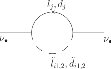
Figure 1: Diagrams by which neutrino masses are generated at the one loop level by the trilinear $R$-parity violating superpotential interactions in (8).

Loops with third generation leptons/quarks yield the largest entries, and the corresponding scale of the neutrino mass is given by,

$$m_{\nu}\sim\frac{\lambda\cdot\lambda}{32\pi^{2}}\sin 2\theta_{\tau}m_{\tau}\ \ {\rm or}\ \ \frac{\lambda^{\prime}\cdot\lambda^{\prime}}{32\pi^{2}}\sin 2\theta_{b}m_{b},$$ (10)

where $\lambda$ and $\lambda^{\prime}$ denote the appropriate $\lambda_{ijk}$ or $\lambda^{\prime}_{ijk}$ coupling, and $\theta_{\tau},\theta_{b}$ are the intragenerational mixing angles for tau sleptons and bottom squarks, respectively. Since $\sin 2\theta_{f}\sim{m_{f}\over M_{\rm SUSY}}\sim 10^{-2}$ for $f=b,\tau$, we see that we can obtain a neutrino mass scale of 0.1 eV (which is consistent with all data) if $\lambda,\lambda^{\prime}\sim 10^{-3}$.

In keeping with our stated philosophy, a coupling of this magnitude requires explanation. We may envision that these couplings, which are forbidden at the tree-level by the $U(1)^{\prime}$ symmetry, may be induced by $vev$s of the scalar components of superfields $\hat{Y}$ that enter the superpotential through,

$$\hat{W}\ni\frac{\hat{Y}_{1}}{M_{P}}\hat{L}\hat{L}\hat{E}^{c}+\frac{\hat{Y}_{2}}{M_{P}}\hat{Q}\hat{L}\hat{D}^{c}.$$ (11)

This would require $\langle Y_{i}\rangle\sim 10^{15}$ GeV, four orders of magnitude larger than the scale $10^{11}$ GeV for the $vev$s of the fields neeeded to solve the $\mu$ problem. While the existence of such fields cannot be logically excluded, since they are not needed for anything, we may consistently assume that these are absent. In this case, we may expect that $\lambda,\ \lambda^{\prime}\sim\frac{\Lambda}{M_{P}}\sim 10^{-7}$ (or even smaller if the symmetry requires higher powers of the MSSM singlet field). The contributions to active neutrino masses from these couplings is then completely negligible, at least as far as their measured oscillation parameters are concerned.

We will see below that the field $\hat{Z}^{\prime}$ that we introduce along with $\hat{Z}$ to solve the $\mu$ and $b_{\mu}$ problems, simultaneously plays the role of the field $\hat{X}$ that sets the mass scale in the active neutrino sector. Radiative corrections then allow us to accommodate (though not explain) the required pattern of neutrino masses and mixing angles.

III The complete model

We have just seen that in addition to a hidden sector superpotential $\hat{W}_{0}$ that we need to break supersymmetry at an intermediate scale $\Lambda\sim 10^{11}$ GeV, we have to introduce new superfields that we will call $\hat{X}_{1}$ and $\hat{X_{2}}$ that acquire $vev$s $\sim\Lambda$ for their scalar components, and $\sim{\Lambda^{3}\over M_{P}}$ for their auxiliary components. The field $\hat{X}_{2}$ plays a dual role in that it not only induces the SUSY breaking $vev$ for ${\cal F}_{X_{1}}$ that we need for the Kim-Nilles mechanism KNM , but also sets the mass scale for active neutrinos. We begin by exhibiting a model that leads to this required pattern of $vev$s for the fields $\hat{S}$ and $\hat{X}_{1,2}$.

III.1 Dynamical origin of the vaccum expectation values

We begin by introducing the superpotential,

$$\hat{W}=\frac{\Lambda^{2}}{M_{P}^{2}}[M_{P}^{2}\hat{S}+\alpha M_{P}\hat{S}^{2}+\beta\hat{S}^{3}+\gamma M_{P}^{3}]+\frac{\kappa}{M_{P}}\hat{X}_{1}^{3}\hat{X}_{2}+\cdots.$$ (12)

The first term is just $\hat{W}_{0}$ that we have introduced earlier. The second term shows the lowest dimensional interaction involving the fields $\hat{X}_{1,2}$ (that we introduce to dynamically generate the $\mu$ and $b_{\mu}$ parameters as described in Sec. II.3) invariant under the $U(1)^{\prime}$ gauge symmetry. The corresponding coupling constant $\kappa\sim 1$. We will see below that this term is essential in that if $\kappa=0$, we will have only supersymmetric solutions. The ellipses include superpotential couplings of $\hat{X}_{1}$ to the fields $\hat{H}_{u,d}$, of $\hat{X_{2}}$ to $\hat{L}_{i}$ and $\hat{H}_{u}$ and $\hat{W}_{\rm MSSM}$ that are unimportant for our analysis of the $vev$s of $\hat{S}$ and $\hat{X}_{1,2}$. The Kähler potential takes the minimal form,

$$\hat{K}=\hat{S}^{\dagger}\hat{S}+\hat{X}_{1}^{\dagger}\hat{X}_{1}+\hat{X}_{2}^{\dagger}\hat{X}_{2}+\hat{\Phi}_{i}^{\dagger}\hat{\Phi}_{i}+\cdots,$$ (13)

consistent with the assumed symmetries. The ellipses denote higher dimensional terms such as $\frac{(\hat{S}+\hat{S}^{\dagger})^{n}}{M_{P}^{n}}\hat{X}_{i}^{\dagger}\hat{X}_{i}$, as well as similar terms involving MSSM superfields that are consistent with the assumed symmetries. These higher dimensional terms are undoubtedly present, but will only give ${\cal O}(1)$ corrections to the solutions that we will obtain for the $vev$s, that do not qualitatively change the different scales that we obtained by our analysis. Finally, to obtain weak scale masses for gauginos, we choose the gauge kinetic function to be given by (3). Again, higher powers of ${\hat{S}\over M_{P}}$ that may be present in the gauge kinetic function will not qualitatively alter our solution.

To facilitate our calculation of the $vev$s for the scalar components of $\hat{S}$ and $\hat{X}_{1,2}$, we evaluate the relevant portion of the scalar potential for our model by substituting the superpotential (12) along with our choice of the Kähler potential and the gauge kinetic function into (4) to obtain,

$$V = \Lambda^{4}\left[V_{0}(\alpha,\beta,\gamma,\frac{S}{M_{P}})+\frac{\Lambda^{2}}{M_{P}^{2}}V_{1}(\alpha,\beta,\gamma,\kappa,\frac{S}{M_{P}},\frac{X_{1}}{\Lambda},\frac{X_{2}}{\Lambda})\right.$$ (14)

$$+\left.\frac{\Lambda^{4}}{M_{P}^{4}}V_{2}(\alpha,\beta,\gamma,\kappa,\frac{S}{M_{P}},\frac{X_{1}}{\Lambda},\frac{X_{2}}{\Lambda})+\cdots\right]e^{K/M_{P}^{2}}$$

$$+\frac{g^{\prime 2}}{2}\Lambda^{4}\left(1+f\frac{S}{M_{P}}\right)^{-1}\left[{\cal X}_{1}\frac{X_{1}X_{1}^{*}}{\Lambda^{2}}+{\cal X}_{2}\frac{X_{2}X_{2}^{*}}{\Lambda^{2}}\right]^{2},$$

where $K$ (without the caret) is the value of the Kähler potential, with the superfields replaced by their scalar components. For simplicity, we have taken $\alpha,\beta,\gamma,\kappa$ to be real parameters. Also, $g^{\prime}$ that appears in the $D$-term contribution to the potential is the gauge coupling strength for the new U(1)^′ group. Finally, ${\cal X}_{1,2}$ denote the $U(1)^{\prime}$ charges of the fields $\hat{X}_{1,2}$: these evidently must satisfy $3{\cal X}_{1}=-{\cal X}_{2}$ in order for the superpotential to be $U(1)^{\prime}$ invariant.

Keeping in mind that our goal is to show that this potential allows (classical) minima with $\langle S\rangle\sim M_{P}$, $\langle X_{1,2}\rangle\sim\Lambda$ with $\langle\Phi_{i}\rangle\ll\Lambda$, we have written the scalar potential in terms of appropriately scaled fields ${S\over M_{P}}$ and ${X_{1,2}\over\Lambda}$, and left out terms in the observable fields $\Phi_{i}$ in (14). Although we have no dynamical argument for selecting this vacuum solution, it is clearly the only one that can lead to a viable phenomenology. The dimensionless functions $V_{0},V_{1},V_{2}$ and $K/M_{P}^{2}$ are then all ${\cal O}$(1) and the scalar potential itself is ${\cal O}(\Lambda^{4})$. Indeed, (14) is an expansion of the scalar potential with each successive term being smaller in magnitude by a factor ${\Lambda^{2}\over M_{P}^{2}}$. The ellipses denote yet higher order terms. The observable sector fields (that we have not written) would enter via the functions $V_{2}$, $V_{3}$, $\cdots$, and also via suppressed terms in the square parenthesis in the last term of (14). Fortunately, these terms only result in tiny corrections to the $vev$s of the scalar components of $\hat{S}$ and $\hat{X}_{1,2}$, and can be neglected in our analysis. The functions $V_{0}$ and $V_{1}$ are given by,

$$V_{0}(\alpha,\beta,\gamma,\frac{S}{M_{P}}) = f_{s}f_{s}^{*}-3W_{s}W_{s}^{*}$$

$$V_{1}(\alpha,\beta,\gamma,\kappa,\frac{S}{M_{P}},\frac{X_{1}}{\Lambda},\frac{X_{2}}{\Lambda}) = (f_{s}^{*}\frac{S^{*}}{M_{P}}-3W_{s}^{*})\kappa\frac{X_{1}^{3}}{\Lambda^{3}}\frac{X_{2}}{\Lambda}+{\rm c.c.}$$ (15)

$$+\left(3\kappa\frac{X_{1}^{2}}{\Lambda^{2}}\frac{X_{2}}{\Lambda}+W_{s}\frac{X_{1}^{*}}{\Lambda}\right)\left(3\kappa\frac{X_{1}^{2}}{\Lambda^{2}}\frac{X_{2}}{\Lambda}+W_{s}\frac{X_{1}^{*}}{\Lambda}\right)^{*}$$

$$+\left(\kappa\frac{X_{1}^{3}}{\Lambda^{3}}+W_{s}\frac{X_{2}^{*}}{\Lambda}\right)\left(\kappa\frac{X_{1}^{3}}{\Lambda^{3}}+W_{s}\frac{X_{2}^{*}}{\Lambda}\right)^{*},$$

where

$$f_{s} = {\cal F}_{S}/\Lambda^{2},\ \ \ {\rm with}$$

$${\cal F}_{S} = \frac{\partial W_{S}}{\partial S}+\frac{W_{S}}{M_{P}^{2}}\frac{\partial K}{\partial S},$$ (16)

$$W_{s} = \frac{1}{M_{P}^{3}}[M_{P}^{2}S+\alpha M_{P}S^{2}+\beta S^{3}+\gamma M_{P}^{3}].$$

In addition to the extremization conditions,

$$\frac{\partial V}{\partial(S/M_{P})}=\frac{\partial V}{\partial(X_{1}/\Lambda)}=\frac{\partial V}{\partial(X_{2}/\Lambda)}=0,$$

(17)

for the fields $S$ and $X_{1,2}$, we require that

$$\langle V\rangle=0,\quad\langle{\cal F}_{S}\rangle\neq 0,$$ (18)

so that the cosmological constant vanishes (to the order that we are evaluating it) and that supersymmetry is broken. We further require that there are no tachyonic directions after we have shifted the fields by their vacuum expectation values; i.e the squared scalar mass parameters are non-negative.

We can satisfy these conditions order-by-order in powers of $\Lambda^{2}$. Specifically, we show that for a given choice of $\langle S\rangle\sim M_{P}$ and $\langle X_{1,2}\rangle\sim\Lambda$, it is possible to choose the model parameters $\alpha,\ \beta,\ \gamma$ all ${\cal O}(1)$, so that (17) and (18) are satisfied. Toward this end, we write,

$$\frac{\langle S\rangle}{M_{P}} = a_{0}+a_{1}\frac{\Lambda^{2}}{M_{P}^{2}}+a_{2}\frac{\Lambda^{4}}{M_{P}^{4}}+\cdots,$$

$$\frac{\langle X_{1}\rangle}{\Lambda} = b_{0}+b_{1}\frac{\Lambda^{2}}{M_{P}^{2}}+b_{2}\frac{\Lambda^{4}}{M_{P}^{4}}+\cdots,$$

$$\frac{\langle X_{2}\rangle}{\Lambda} = c_{0}+c_{1}\frac{\Lambda^{2}}{M_{P}^{2}}+c_{2}\frac{\Lambda^{4}}{M_{P}^{4}}+\cdots,$$

$$\alpha = \alpha_{0}+\alpha_{1}\frac{\Lambda^{2}}{M_{P}^{2}}+\alpha_{2}\frac{\Lambda^{4}}{M_{P}^{4}}+\cdots,$$

$$\beta = \beta_{0}+\beta_{1}\frac{\Lambda^{2}}{M_{P}^{2}}+\beta_{2}\frac{\Lambda^{4}}{M_{P}^{4}}+\cdots,$$

$$\gamma = \gamma_{0}+\gamma_{1}\frac{\Lambda^{2}}{M_{P}^{2}}+\gamma_{2}\frac{\Lambda^{4}}{M_{P}^{4}}+\cdots,$$ (19)

where the coefficients $a_{\bullet}$’s, $b_{\bullet}$’s, $\cdots$ $\gamma_{\bullet}$’s are all are ${\cal O}$(1). If we work to leading order, i.e. drop all terms ${\cal O}(\Lambda^{4}\times\frac{\Lambda^{2}}{M_{P}^{2}})$, it is clear that we must separately minimize the first and last terms of (14), and also satisfy (18). Minimization of the $D$-term contribution to the scalar potential then gives us (we take the $vev$s to be real),

$${\cal X}_{1}\frac{\langle X_{1}\rangle^{2}}{\Lambda^{2}}+{\cal X}_{2}\frac{\langle X_{2}\rangle^{2}}{\Lambda^{2}}=0,\ \ \ {\rm or}\ 3{\cal X}_{1}=-{\cal X}_{2}.$$ (20)

Extremization with respect to $S$ and the vanishing of the cosmological constant then give,

$$(\langle f_{s}\rangle^{2}-3\langle W_{s}\rangle^{2})e^{K/M_{P}^{2}}=0,\quad\frac{\partial(V_{0}e^{K/M_{P}^{2}})}{\partial(S/M_{P})}=0.$$ (21)

It is clear that for given values of $a_{0}$, $b_{0}$ and $c_{0}$, we can always choose two of the three parameters $\alpha_{0}$, $\beta_{0}$ and $\gamma_{0}$ to satisfy these conditions.

While the ratio ${\langle X_{1}\rangle}\over{\langle X_{2}\rangle}$ is fixed even at leading order, the scale of $\langle X_{1,2}\rangle$ is still arbitrary. This degeneracy of the potential is removed once we take the terms $\sim\Lambda^{6}/M_{P}^{2}$ that appear in $V_{1}$ into account. The extremization conditions then give us,

$$\left(\frac{\langle X_{2}\rangle}{M_{P}}\right)\left[81\left(\frac{\kappa\langle X_{2}\rangle^{2}}{\Lambda^{2}}\right)^{2}+3\sqrt{3}\left(\langle f_{s}\rangle\frac{\langle S\rangle}{M_{P}}+\langle W_{s}\rangle\right)\frac{\kappa\langle X_{2}\rangle^{2}}{\Lambda^{2}}+\langle W_{s}\rangle^{2}\right]=0.$$ (22)

We obtain non-vanishing values of $\langle X_{2}\rangle$ if the second factor vanishes. Substituting $f_{s}=\sqrt{3}W_{s}$ from the first equation in (21), we see that we obtain real solutions for $\langle X_{2}\rangle$ provided,

$$\left|\frac{\langle S\rangle}{M_{P}}\right|\geq 2-\frac{1}{\sqrt{3}}\approx 1.42.$$ (23)

The reader may be concerned that we are assuming the effective theory assumed to be valid below the Planck scale to derive Planck scale $vev$s for which yet higher powers of $\hat{S}$ in $\hat{W}_{0}$ (these are not forbidden by any symmetry) may be important. Moreover, the superpotential could also include terms such as $\frac{\hat{S}^{n}}{M_{P}^{n}}\times\frac{\hat{X}_{1}^{3}\hat{X}_{2}}{M_{P}}$ (as well as corresponding terms involving MSSM superfields) that would, for large enough $n$, destabilize $\kappa$ in (12) from its value of ${\cal O}(1)$, if $\langle S\rangle>M_{P}$. The point, however, is that none of our conclusions from this point on will depend on the choice of $\hat{W}_{0}$. The rest of our analysis (which determines the observable particle physics) would be qualitatively unchanged even if $\hat{W}_{0}$ is not a polynomial and radiative corrections are included, as long as $\langle S\rangle\sim M_{P}$. Thus, while the precise value of the $vev$ is not trustworthy, our conclusions about various scales arrived at using the fact that $\langle S\rangle\sim M_{P}$ are reliable. Put somewhat differently, we have assumed that the potential of the high energy theory has a local minimum (our vaccuum), with a SUSY breaking scale $\Lambda\ll M_{P}$ and a cosmological constant that is fine-tuned to be (almost) zero, sufficiently separated from other minima. An expansion about this minimum, (rather than about $S=0$) then leads to an effective field theory in which the higher dimensional operators will indeed all be suppressed by corresponding powers of $M_{P}$.

We now have to check whether the extremum that we have obtained is indeed a local minimum. Toward this end, in Table 1 we give an illustrative example of a solution for $\langle S\rangle=1.5M_{P}$. The spontaneous breakdown of the $U(1)^{\prime}$ gives a massless would-be Goldstone boson (a linear combination of the imaginary components of the $X_{1,2}$ fields) that makes the $U(1)^{\prime}$ gauge field massive via the Higgs mechanism. A corresponding combination of the real parts of $X_{1}$ and $X_{2}$ acquire a large mass $m_{Xh}\sim\Lambda$, the precise value depends on the details including parameters in the gauge kinetic function. The corresponding orthogonal combination $X_{l}$ ($h$ and $l$ here denote heavy and light) as well as the non-Goldstone combination of $X_{1I}$ and $X_{2I}$ get masses $\sim(2-20)\Lambda^{2}/M_{P}$ from the interactions contained in the $V_{1}$ part of the scalar potential (14). The real and imaginary parts of the singlet $S$ also acquire TeV scale masses. The positive values of the squared mass parameters indeed demonstrate that we have a true minimum. We remark that for solutions at the lower extreme $\left|\frac{\langle S\rangle}{M_{P}}\right|=2-\frac{1}{\sqrt{3}}$, $m_{Xl}^{2}=0$, so that the state $X_{l}$ which may be very light, could have implications for Higgs physics as well as for cosmology.

$a_{0}$	$\gamma_{0}$	$\kappa b_{0}^{2}$	$\alpha_{0}$	$\beta_{0}$	$\langle{\cal F}_{S}\rangle$	$m_{SR}^{2}$	$m_{SI}^{2}$	$m_{Xh}^{2}$	$m_{Xl}^{2}$	$m_{XI}^{2}$
					$(\Lambda^{2})$	$(\frac{\Lambda^{4}}{M_{P}^{2}})$	$(\frac{\Lambda^{4}}{M_{P}^{2}})$	$(\Lambda^{2})$	$(\frac{\Lambda^{4}}{M_{P}^{2}})$	$(\frac{\Lambda^{4}}{M_{P}^{2}})$
1.5	-.35	-.053	-.44	.059	.63	5.6	14.4	$\sim$1	7.4	54.8
1.5	-.2	-.106	-.21	-.029	1.26	15.5	64.8	$\sim$1	29.7	219.4
1.5	-.1	-.14	-.059	-.088	1.67	8.25	134	$\sim$1	52.7	390
1.5	-.05	-.16	.017	-.118	1.88	2.49	177.6	$\sim$1	66.7	493.6

Table 1: Sample solutions with zero vaccum energy and local minima along with the leading values of the parameters in (19). We have also given SUSY breaking parameter ${\cal F}_{S}$ in units of $\Lambda^{2}$ and also the squared masses of the various scalar fields in units of either $\Lambda^{2}$ or $(\Lambda^{2}/M_{P})^{2}$ as appropriate. As discussed in the text, the corresonding solution for $\langle S\rangle=-1.5M_{P}$ has an identical spectrum.

III.2 Anomalies

Since our solutions to the $\mu$ and $b_{\mu}$ problem, as well as the mechanism for neutrino masses discussed in Sec. II.4, both require us to extend the gauge group, we need to ensure that the associated anomalies cancel. We will see shortly that this will require us to introduce new fields (some of which are charged under the MSSM gauge group, $SU(3)_{C}\times SU(2)_{L}\times U(1)_{Y}$) that may manifest themselves as exotic particles at the multi-TeV scale anomaly ; ma2 .

We note that the invariance of the usual quark Yukawa coupling terms in the superpotential require that

$$2{\cal Q}+{\cal U}^{c}+{\cal D}^{c}+{\cal H}_{u}+{\cal H}_{d}=0,$$ (24)

with the understanding that the calligraphic symbol for the field denotes its $U(1)^{\prime}$ charge. Since an important role of the $U(1)^{\prime}$ field was to forbid the $\mu$ term, we know that ${\cal H}_{u}+{\cal H}_{d}\not=0$, from which we infer that

$$2{\cal Q}+{\cal U}^{c}+{\cal D}^{c}\not=0.$$ (25)

We commence our discussion of the anomalies by observing that the new fields $\hat{S}$ and $\hat{X}_{1,2}$ are $SU(3)_{C}\times SU(2)_{L}\times U(1)_{Y}$ singlets, and so do not spoil the anomaly cancellation of the MSSM. We thus need to focus only on the mixed anomalies involving the MSSM gauge group or gravity and the new $U(1)^{\prime}$ gauge group. We begin with the cancellation of the $[SU(3)_{C}]^{2}\times U(1)^{\prime}$ anomaly which, with the field content that we have up to this point, would require

$$2{\cal Q}+{\cal U}^{c}+{\cal D}^{c}=0,$$

in direct contradiction with (25). We are thus led to introduce new $SU(2)_{L}$ singlet, colour triplet fields $\hat{K}$ and $\hat{K}^{\prime}$ in the ${\bf 3}$ and ${\bf 3}^{*}$ representation of $SU(3)_{C}$ with $U(1)^{\prime}$ quantum numbers ${\cal K}$ and ${\cal K}^{\prime}$, respectively, and weak hypercharge $y(K)=-y(K^{\prime})$. Since $\hat{K}$ and $\hat{K}^{\prime}$ are in conjugate representations of the MSSM gauge group, their introduction does not affect the cancellation of the $SU(3)_{C}\times SU(2)_{L}\times U(1)_{Y}$ and the mixed $[gravity]^{2}-U(1)_{Y}$ anomalies. We choose their $U(1)^{\prime}$ charges to cancel the mixed $[SU(3)_{C}]^{2}\times U(1)^{\prime}$ anomaly. However, we also need to ensure that the coloured superfields acquire a mass. The simplest way to do so is to introduce a superpotential coupling

$$\hat{W}\ni\frac{\hat{X}_{1}^{2}\hat{K}\hat{K}^{\prime}}{M_{P}}$$

which is consistent with the cancellation of the anomaly provided we introduce one pair of $\hat{K}$ and $\hat{K}^{\prime}$ for each matter family. To understand the reason for this, we first note that the cancellation of the $[SU(3)_{C}]^{2}\times U(1)^{\prime}$ anomaly then requires that,

$$[SU(3)_{C}]^{2}-U(1)^{\prime} :\quad 3(2{\cal Q}+{\cal U}^{c}+{\cal D}^{c})+\sum_{i=1}^{n_{K}}\left({\cal K}_{i}+{\cal K}^{\prime}_{i}\right)=0,$$ (26)

where the factor 3 on the first term on the right-hand-side arises because there are three quark families, and the index $i=1-n_{K}$ counts different sets of $\hat{K}$ and $\hat{K}^{\prime}$ fields (with the same $U(1)^{\prime}$ quantum numbers). Since our solution to the $\mu$ and $b_{\mu}$ problems requires that ${\cal H}_{u}+{\cal H}_{d}=-2{\cal X}_{1}$, we infer from (26) that the lowest dimensionality $U(1)^{\prime}$-invariant superpotential operator that can give the new coloured fields a mass is $\hat{X}_{1}^{\frac{6}{n_{K}}}\hat{K}\hat{K}^{\prime}$, where $n_{K}=1,3$ or 6, is the number of pairs of these coloured fields. The corresponding mass for these fields is $\sim{{\Lambda^{\frac{6}{n_{K}}}}\over{M_{P}^{{\frac{6}{n_{K}}}-1}}}$, which for $\Lambda\sim 10^{11}$ GeV is unacceptably small for $n_{K}=1$ but leads to the interesting prediction of new coloured states at the multi-TeV scale if $n_{K}=3$ is the number of quark generations.

The superpotential, for quarks, leptons, Higgs and the new superfields that various considerations have led us to introduce, must include

$$\hat{W}\ni{\bf Y}^{u}_{ij}\hat{Q}_{i}\hat{U}^{c}_{j}\hat{H}_{u}+{\bf Y}^{d}_{ij}\hat{Q}_{i}\hat{D}^{c}_{j}\hat{H}_{d}+{\bf Y}^{e}_{ij}\hat{L}_{i}\hat{E}^{c}_{j}\hat{H}_{d}+a\frac{\hat{X}_{1}^{2}}{M_{P}}\hat{H}_{u}\hat{H}_{d}+a^{\prime}\frac{\hat{X}_{1}^{3}\hat{X}_{2}}{M_{P}}+h_{i}\frac{\hat{X}_{2}^{3}}{M_{P}^{2}}\hat{L}_{i}\hat{H}_{u}+a^{{}^{\prime\prime}}_{i}\frac{\hat{X}_{1}^{2}}{M_{P}}\hat{K}_{i}\hat{K}^{\prime}_{i}+\cdots,$$ (27)

where ${\bf Y}$’s are the usual quark and lepton Yukawa coupling matrices, and $a$, $a^{\prime}$, $a^{{}^{\prime\prime}}_{i}$ and $h_{i}$ are dimensionless coupling constants assumed to be ${\cal O}$(1), and a sum over the indices $i$ and $j$ is implied. The penultimate term leads to neutrino masses as discussed in Sec. II.4. The last term in (27), that gives supersymmetric masses to the $\hat{K}_{i}$ and $\hat{K}^{\prime}_{i}$ has been written in the diagonal basis for these fields. The ellipses include yet higher dimensional operators in the superpotential that would be allowed by the gauge symmetry but are of no relevance to us, along with the dynamics of the SUSY-breaking singlet $\hat{S}$ that we have already discussed.

The conditions for the cancellation of the remaining gauge and mixed gauge-gravity anomalies that supplement (26) above read,

$$[SU(2)_{L}]^{2}-U(1)^{\prime} :\quad 9{\cal Q}+3{\cal L}+{\cal H}_{u}+{\cal H}_{d}=0,$$ (32)

$$[U(1)_{Y}]^{2}-U(1)^{\prime} :\quad 2{\cal Q}+16{\cal U}^{c}+4{\cal D}^{c}+3(2{\cal L}+4{\cal E}^{c})+2{\cal H}_{d}+2{\cal H}_{u}$$

$$+3\sum_{i=1}^{3}\left(y(K_{i})^{2}{\cal K}_{i}+y(K^{\prime}_{i})^{2}{\cal K}^{\prime}_{i}\right)=0,$$

$$[\rm gravity]^{2}-U(1)^{\prime} :\quad 9(2{\cal Q}+{\cal U}^{c}+{\cal D}^{c})+3(2{\cal L}+{\cal E}^{c})+2({\cal H}_{d}+{\cal H}_{u})+N_{1}{\cal X}_{1}+N_{2}{\cal X}_{2}$$

$$+N_{3}{\cal Y}_{1}+N_{4}{\cal Y}_{2}+3\sum_{i=1}^{3}\left({\cal K}_{i}+{\cal K}^{\prime}_{i}\right)=0,$$

$$U(1)_{Y}-[U(1)^{\prime}]^{2} :\quad 3(2{\cal Q}^{2}-4{\cal U}^{c2}+2{\cal D}^{c2})+3(-2{\cal L}^{2}+2{\cal E}^{c2})+2(-{\cal H}^{2}_{d}+{\cal H}^{2}_{u})$$

$$+3\sum_{i=1}^{3}\left(y(K_{i}){\cal K}^{2}_{i}+y(K^{\prime}_{i}){\cal K}^{\prime 2}_{i}\right)=0,\ \ \ {\rm and}$$

$$[U(1)^{\prime}]^{3} :\quad 9(2{\cal Q}^{3}+{\cal U}^{c3}+{\cal D}^{c3})+3(2{\cal L}^{3}+{\cal E}^{c3})+2({\cal H}^{3}_{d}+{\cal H}^{3}_{u})+N_{1}{\cal X}^{3}_{1}+N_{2}{\cal X}^{3}_{2}$$

$$+N_{3}{\cal Y}^{3}_{1}+N_{4}{\cal Y}^{3}_{2}+3\sum_{i=1}^{3}\left({\cal K}^{3}_{i}+{\cal K}^{\prime 3}_{i}\right)=0.$$

The reader will have to notice that we have included two additional $SU(3)_{C}\times SU(2)_{L}\times U(1)_{Y}$ singlet superfields $\hat{Y}_{1}$ and $\hat{Y_{2}}$ with non-trivial $U(1)^{\prime}$ charges that do not alter anomalies involving any SM gauge boson in our analysis. As we will see below, their inclusion is only necessary if we want to obtain rational values for all $U(1)^{\prime}$ charges. We have also allowed for several copies ($N_{1},\ N_{2},\ N_{3},\ N_{4}$) of the SM singlet superfields ($\hat{X}_{1},\ \hat{X}_{2},\ \hat{Y}_{1},\ \hat{Y}_{2}$, respectively). We must thus understand that the couplings $a$, $a^{\prime}$, $a^{{}^{\prime\prime}}$ as well as the coupling $h_{i}$ that appear in (27) carry an extra index that specifies just which one of these multiple singlet fields we are referring to.

The various $U(1)^{\prime}$ charges are, of course, not independent since the corresponding invariance of $\hat{W}$ in (27) requires that,

$${\cal Q}+{\cal U}^{c}+{\cal H}_{u}=0,$$ (33)

$${\cal Q}+{\cal D}^{c}+{\cal H}_{d}=0,$$ (34)

$${\cal L}+{\cal E}^{c}+{\cal H}_{d}=0,$$ (35)

$$2{\cal X}_{1}+{\cal H}_{d}+{\cal H}_{u}=0,$$ (36)

$$3{\cal X}_{2}+{\cal L}+{\cal H}_{u}=0,$$ (37)

$$2{\cal X}_{1}+{\cal K}_{i}+{\cal K}^{\prime}_{i}=0,$$ (38)

$${\cal X}_{2}+3{\cal X}_{1}=0.$$ (39)

Notice that we can eliminate ${\cal H}_{u}$, ${\cal H}_{d}$ and ${\cal X}_{1}$ from (33), (34), (36) and (38) to obtain (26). The other equations are all independent and, along with the ratio ${\cal Y}_{1}/{\cal X}_{1}$ which is fixed to obtain rational values of $U(1)^{\prime}$ charges as discussed below, can be used to write the $U(1)^{\prime}$ charges of the seventeen fields (up to discrete quadratic or cubic ambiguities) in terms of the charges of any two fields which we will take to be ${\cal X}_{1}$ and ${\cal L}$. Our aim is to display one such solution explicitly.

Toward this end, we remark that by considering the linear combination

$$\frac{1}{2}\times(29)+(28)-8\times(33)-2\times(34)-6\times(35),$$

of equations (32), (32), (33), (34) and (35), and noting that ${\cal H}_{u}+{\cal H}_{d}=-2{\cal X}_{1}={\cal K}_{i}+{\cal K}_{i}^{\prime}$, we obtain (since ${\cal X}_{1}\not=0$)

$$\sum_{i=1}^{3}y(\hat{K}_{i})^{2}=4.$$ (40)

This choice of weak hypercharges is necessary to guarantee the cancellation of the $[U(1)_{Y}]^{2}-U(1)^{\prime}$ anomaly.

Next, in (32) for the cancellation of the $[{\rm gravity}]^{2}-U(1)^{\prime}$ anomaly, we first note that the first and last terms sum to zero. Then, using (35)–(37) together with ${\cal X}_{2}=-3{\cal X}_{1}$, we find that,

$$(N_{1}-3N_{2}+29){\cal X}_{1}+N_{3}{\cal Y}_{1}+N_{4}{\cal Y}_{2}=0,$$ (41)

which shows why multiple copies of some of these MSSM singlet fields are necessary. A simple solution is given by,

$$N_{1}=1,\quad N_{2}=10,\quad{\cal X}_{2}=-3{\cal X}_{1},$$

$$N_{3}=1,\quad N_{4}=2,\quad{\cal Y}_{1}=-2{\cal Y}_{2}.$$ (42)

We now turn to the last two anomaly constraints, the quadratic and cubic equations, (32) and (32), for the $U(1)^{\prime}$ charges. These depend explicitly on the weak hypercharges of the fields $\hat{K}_{i}$ which, as we have seen, satisfy (40). Of the many possible solutions, we first make the simple choice $y(\hat{K}_{i})=(2,0,0)$ which obviously leads to integrally charged, coloured particles. To find a solution, we first use (33)–(39) together with (32) to eliminate all $U(1)^{\prime}$ charges in terms of ${\cal X}_{1}$, ${\cal L}$ and ${\cal K}_{1}$, and then plug these into (32) to obtain (note that ${\cal K}_{2}$ and ${\cal K}_{3}$ drop out because the corresponding weak hypercharges are chosen to be zero),

$$\frac{8}{3}{\cal X}_{1}(-9{\cal L}+56{\cal X}_{1})-12{\cal X}_{1}{\cal K}_{1}=0.$$ (43)

Finally, we turn to the $[U(1)^{\prime}]^{3}$ anomaly equation (32). Writing all but ${\cal K}_{i}$ and ${\cal Y}_{1}$ in terms of ${\cal L}$ and ${\cal X}_{1}$ (remember that ${\cal Y}_{1}=-2{\cal Y}_{2}$), this reduces to,

$$\sum_{i=1}^{3}{\cal K}_{i}^{2}+2{\cal X}_{1}{\cal K}_{i}=\frac{1}{18{\cal X}_{1}}\{72{\cal L}^{2}{\cal X}_{1}-968{\cal L}{\cal X}_{1}^{2}+\frac{19970}{3}{\cal X}_{1}^{3}+\frac{3}{4}{\cal Y}_{1}^{3}\}.$$ (44)

We now eliminate ${\cal K}_{1}$ using (43) and find,

$$({\cal K}_{2}+{\cal X}_{1})^{2}+({\cal K}_{3}+{\cal X}_{1})^{2}=\left(\frac{{\cal X}_{1}}{9}\right)^{2}\left[15557+\left(\frac{3{\cal Y}_{1}}{2{\cal X}_{1}}\right)^{3}\right].$$ (45)

Remarkably, ${\cal L}$ does not appear in this equation, which has solutions with rational values of $U(1)^{\prime}$ charges for $\frac{3{\cal Y}_{1}}{2{\cal X}_{1}}=-1$, $-3$, $-4$, $-6$, $-10,\cdots$. We now see the role of the $\hat{Y}_{1,2}$ fields. Without these, the anomaly constraints would be satisfied, only for irrational values of the $U(1)^{\prime}$ charges, precluding the possibility of embedding the model into a grand unified framework with a simple gauge group.

We note that it is also possible to satisfy the anomaly equations with $y(\hat{K}_{i})=\left(\frac{2}{3},\frac{4}{3},\frac{4}{3}\right)$ which leads to electric charges $\pm\frac{1}{3}$ or $\pm\frac{2}{3}$ for the coloured $\hat{K}_{i}$ and $\hat{K}^{\prime}_{i}$ fields. Again solutions are possible for $\frac{3{\cal Y}_{1}}{2{\cal X}_{1}}=-1$, $-3$, $-4$, $-6$, $-10,\cdots$. In this case, the reader may suppose that the new coloured particles may mix (upon spontaneous breaking of $U(1)^{\prime}$) with the usual $SU(2)$-singlet quarks and squarks with the same spin and electric charge. However, as we will see below, there are simple cases where such mixing is precluded.

To recapitulate, the requirement of anomaly cancellation forces us to introduce three pairs of coloured fields $\hat{K}_{i}$ and $\hat{K}_{i}^{\prime}$, with either integral or fractional electric charges, with masses at the TeV scale. We also require SM singlet superfields $\hat{X}_{1,2}$ and $\hat{Y}_{1,2}$, with ten copies of $\hat{X_{2}}$ and two of $\hat{Y}_{2}$. The $\hat{Y}_{1,2}$ fields are necessary only if we insist on rational values of $U(1)^{\prime}$ charges. There are many solutions to the anomaly equations. Here, we exhibit an explicit solution with $\frac{3{\cal Y}_{1}}{2{\cal X}_{1}}=-22$, for which the new $U(1)^{\prime}$ charges are fixed by the corresponding charges of $\hat{X}_{1}$ and $\hat{L}_{i}$ fields by,

$${\cal X}_{2}=-3{\cal X}_{1},\quad{\cal Y}_{1}=-\frac{44}{3}{\cal X}_{1},\quad{\cal Y}_{2}=\frac{22}{3}{\cal X}_{1},$$

$${\cal K}_{1}=\frac{2}{9}(-9{\cal L}+56{\cal X}_{1})\ \left[-\frac{2}{3}{\cal L}-\frac{40}{27}{\cal X}_{1}\right],\quad{\cal K}_{2}=\frac{61}{9}{\cal X}_{1}\ \left[-\frac{4}{3}{\cal L}+\frac{139}{27}{\cal X}_{1}\right],$$

$${\cal K}_{3}=-\frac{2}{3}{\cal X}_{1}\ \left[-\frac{4}{3}{\cal L}+\frac{358}{27}{\cal X}_{1}\right],\quad{\cal K}^{\prime}_{i}=-{\cal K}_{i}-2{\cal X}_{1},\quad i=1,2,3,$$ (46)

$${\cal Q}=(-3{\cal L}+2{\cal X}_{1})/9,\quad{\cal D}^{c}=-\frac{2}{3}{\cal L}+\frac{97}{9}{\cal X}_{1},\quad{\cal U}^{c}=\frac{4}{3}{\cal L}-\frac{83}{9}{\cal X}_{1},$$

$${\cal E}^{c}=-2{\cal L}+11{\cal X}_{1},\quad{\cal H}_{u}=-{\cal L}+9{\cal X}_{1},\quad{\cal H}_{d}={\cal L}-11{\cal X}_{1},$$

where the values of ${\cal K}_{i}$ outside (within) the square parenthesis refer to the integrally (fractionally) charged case for the $\hat{K}_{i}$ fields discussed above. For rational values of ${\cal L},{\cal X}_{1}$, we obtain rational U(1)^′ charges for all the other fields. We have checked that despite the large number of fields that we have introduced, the $U(1)^{\prime}$ gauge coupling does not blow up below $Q=M_{P}$ as long as the corresponding weak scale gauge coupling is smaller than about 0.05 [0.6] for $({\cal L},{\cal X}_{1})$ = (1,1) [(1, 0.1)], i.e. as long as the couplings of fields such as $\hat{E}^{c}$, $\hat{D}^{c}$, etc. that have a much larger coupling to the $U(1)^{\prime}$ gauge boson than $\hat{X}_{1}$, are similar in magnitude to the SM gauge couplings.

The alert reader will have noted that since we chose the weak hypercharges for the colour triplet fields to be positive, it is the charged $\frac{1}{3}$ triplet $\hat{K}_{1}$, not the anti-triplet $\hat{K}_{1}^{\prime}$, that has positive charge. Before closing this discussion, we point out how the $U(1)^{\prime}$ charges in (46) would be altered had we instead chosen the weak hypercharge $y(\hat{K}_{1})=-\frac{2}{3}$. This would have only shown itself only in the $U(1)_{Y}-U(1)^{\prime 2}$ anomaly equation (32), which does not distinguish whether the $\hat{K}_{i}^{(\prime)}$ are triplets or anti-triplets. The flip of the sign of the weak hypercharge of $\hat{K}_{1}$ thus results in an interchange of the $U(1)^{\prime}$ charges of $\hat{K}_{1}$ and $\hat{K}_{1}^{\prime}$ from their values (in the square parenthesis) in (46), with the $U(1)^{\prime}$ charges of all other fields remaining unchanged.

III.3 A recap

With the $U(1)^{\prime}$ charges that we have just obtained in (46), the most general superpotential, invariant under the assumed symmetries, may be written as,

$$W = \frac{\Lambda^{2}}{M_{P}^{2}}[M_{P}^{2}\hat{S}+\alpha M_{P}\hat{S}^{2}+\beta\hat{S}^{3}+\gamma M_{P}^{3}]+\sum_{a=1}^{2}y_{a}\hat{Y}_{1}\hat{Y}^{2}_{2a}+\sum_{b=1}^{10}\frac{\kappa_{b}}{M_{P}}\hat{X}_{1}^{3}\hat{X}_{2b}+Y^{u}_{ij}\hat{Q}_{i}\hat{U}^{c}_{j}\hat{H}_{u}+$$ (47)

$$Y^{d}_{ij}\hat{Q}_{i}\hat{D}^{c}_{j}\hat{H}_{d}+Y^{e}_{ij}\hat{L}_{i}\hat{E}^{c}_{j}\hat{H}_{d}+\frac{\hat{X}_{1}^{2}}{M_{P}}\hat{H}_{u}\hat{H}_{d}+\sum_{b=1}^{10}h_{ib}\frac{\hat{X}_{2b}^{3}}{M_{P}^{2}}\hat{L}_{i}\hat{H}_{u}+a_{i}^{{}^{\prime\prime}}\frac{\hat{X}_{1}^{2}}{M_{P}}\hat{K}_{i}\hat{K}^{\prime}_{i}+\cdots,$$

where a sum over $i,j$ is implied, and $y_{a}$ are couplings of ${\cal O}$(1). Here, we have explicitly shown the sums over the MSSM singlet fields $\hat{X}_{2b}$ and $\hat{Y}_{2a}$, while the sums over the family indices $i$ and $j$ (including for the colour triplet superfields $\hat{K}_{i}$ and $\hat{K}^{\prime}_{i}$) are implied. The ellipses denote other terms allowed by the symmetries, but suppressed by even higher powers of $M_{P}$, that are irrelevant for our analysis.

It is instructive to note that trilinear $R$-parity violating operators,

$$\hat{L}_{i}\hat{L_{j}}\hat{E}^{c}_{k},\ \hat{L}_{i}\hat{Q}_{j}\hat{D}^{c}_{k},\ {\rm and}\ \hat{U}^{c}_{i}\hat{D}^{c}_{j}\hat{D}^{c}_{k},$$

are automatically forbidden by the $U(1)^{\prime}$ gauge symmetry. Since $2{\cal L}+{\cal E}^{c}={\cal L}+{\cal Q}+{\cal D}^{c}=11{\cal X}_{1}$, the first two operators may be induced, by the spontaneous breaking of $U(1)^{\prime}$, via effective terms,

$$\frac{(\hat{X}_{1}^{\dagger})^{2}\hat{X}_{2}^{3}}{M_{P}^{6}}\hat{L}\hat{L}\hat{E}^{c},\frac{(\hat{X}_{1}^{\dagger})^{2}\hat{X}_{2}^{3}}{M_{P}^{6}}\hat{L}\hat{Q}\hat{D}^{c}$$

in the Kähler potential which, because $\langle F_{X_{1}}\rangle\sim\frac{\Lambda^{3}}{M_{P}}$ and $\langle X_{1,2}\rangle\sim\Lambda$, leads to associated dimensionless couplings $\sim\frac{\Lambda^{7}}{M_{P}^{7}}\sim 10^{-49}$ which are utterly negligible. Since ${\cal U}^{c}+2{\cal D}^{c}=\frac{37}{3}{\cal X}_{1}$, the baryon-number violating trilinear superpotential interaction $\hat{U}^{c}_{i}\hat{D}^{c}_{j}\hat{D}^{c}_{k}$ cannot be induced.

IV Phenomenology

IV.1 Proton Decay and $n\bar{n}$ oscillations

We have just seen that the $U(1)^{\prime}$ gauge symmetry that we have introduced automatically suppresses all dimensionless baryon and lepton number violating superpotential couplings to negligible levels. Thus, the introduction of ad hoc global symmetries to avoid the disastrous prediction of proton decay at the weak interaction rate is unnecessary within our model.

The dimension-4 superpotential operators (which generate dimension-5 terms in the interaction Lagrangian),

$$\hat{Q}\hat{Q}\hat{Q}\hat{L}\ {\rm and}\ \hat{U}^{c}\hat{U}^{c}\hat{D}^{c}\hat{E}^{c},$$

can lead to a dangerously high rate for proton decay prodecay . It is, however, easy to see that the $U(1)^{\prime}$ gauge symmetry also forbids these operators. Moreover, these operators are not induced even after $U(1)^{\prime}$ breaking because $3{\cal Q}+{\cal L}=\frac{2}{3}{\cal X}_{1}$, while $2{\cal U}^{c}+{\cal D}^{c}+{\cal E}^{c}=\frac{30}{9}{\cal X}_{1}$. The baryon-number violating (but lepton-number conserving) operator, $\hat{Q}\hat{Q}\hat{Q}\hat{H}_{d}$ is also not possible. We also note that baryon- and lepton-number violating terms,

$$\hat{Q}\hat{Q}\hat{U}^{c\dagger}\hat{E}^{c\dagger}\ {\rm and}\ \hat{Q}\hat{U}^{c\dagger}\hat{D}^{c\dagger}\hat{L},$$

in the Kähler potential, which give rise to gauge-boson-mediated proton decay in many SUSY grand unified theories are also forbidden. Our model is thus safe from constraints from the non-observation of proton decay at Super-Kamiokande superK .

Indeed, it turns out that the proton is stable within this framework. To see this, we first observe that the coefficients multiplying ${\cal L}$ in the $U(1)^{\prime}$ charges in (46) are proportional to the weak hypercharges of the corresponding fields, so that changing just the value of ${\cal L}$ amounts to just a $U(1)_{Y}$ transformation, under which our Lagrangian is automatically invariant. Next, taking ${\cal L}=\frac{2}{3}{\cal X}_{1}$, we observe that the $U(1)^{\prime}$ charges of the MSSM fields, normalized so that ${\cal X}_{1}=3$, are given by,

$$({\cal Q},{\cal U}^{c},{\cal D}^{c},{\cal L},{\cal E}^{c},{\cal H}_{d},{\cal H}_{u},{\cal X}_{1})=(0,-25,31,2,29,-31,25,3)=(0,2,1,2,2,2,1,0)\ {\rm mod}\ 3.$$ (48)

Since only those products of MSSM fields ${\cal O}_{\rm MSSM}$ that are of the form ${\cal O}_{\rm MSSM}\times X_{1}^{(\dagger)n}X_{2}^{(\dagger)m}$ (with $m$ and $n$ being integers) arise in the low energy theory even after spontaneous breakdown of the $U(1)^{\prime}$ group, we conclude that the $U(1)^{\prime}$ charge of ${\cal O}_{\rm MSSM}$ must vanish modulo 3. In other words, a $Z_{3}$ subgroup of $U(1)^{\prime}$ with charges of MSSM fields as in (48) remains as a discrete symmetry of the low energy theory even though $U(1)^{\prime}$ is spontaneously broken. Indeed, this $Z_{3}$ is the same as the discrete symmetry group $B_{3}$ first discussed by Ibañez and Ross IR . The $Z_{3}$ charges of MSSM fields in (48) coincide with the corresponding $2(B-Y)$ charges modulo 3, so that conservation of $Z_{3}$ implies that the $SU(3)_{C}\times SU(2)\times U(1)_{Y}$ invariant low energy effective theory conserves $2B$ modulo 3, or that $\Delta B=1,2$ processes are forbidden cm . The proton is thus stable within our framework, and further, neutron anti-neutron oscillations are also forbidden (or at least very strongly suppressed if $Y_{1}$ or $Y_{2}$ acquires a $Z_{3}$ breaking $vev$).

IV.2 Neutrino sector

We have already seen in Sec. II.4 that because $\hat{X}_{2b}$ fields acquire $vevs$ $\sim\Lambda$, the penultimate term in the superpotential (47) naturally results in a neutrino mass scale $\sim 0.1$ eV. We have also seen that lepton-number-violating trilinear couplings are suppressed to insignificant levels. In the (s)neutrino sector, the TeV scale effective theory is just the MSSM with bilinear $R$-parity violation bilinear contained in the superpotential terms,

$$W_{\rm eff}\ni\epsilon_{i}\epsilon_{ab}\hat{L}_{i}^{a}\hat{H}_{u}^{b},$$ (49)

with $\epsilon_{i}=h_{i}\frac{\langle X_{2}\rangle^{3}}{M_{P}^{2}}\sim 10^{-4}$ GeV, together with the concomitant SSB cousin of the $b_{\mu}$ term,

$$V_{\rm soft}=\epsilon_{ab}b_{\epsilon i}\tilde{L}_{i}^{a}H_{u}^{b}+{\rm c.c.}\;,$$ (50)

where $\tilde{L}_{i}$ denotes the slepton doublet.

The phenomenology of models with bilinear $R$-parity violation, especially as it impacts on the neutrino sector, has been extensively studied in the literature. Here, we will only summarize the salient features. The sneutrino fields acquire $vevs$, $\langle\tilde{\nu}_{i}\rangle\sim\epsilon_{i}\sim 10^{-4}$ GeV, which lead to a mixing between the neutral gauginos and the neutrinos. In other words, we now have a $7\times 7$ neutral gaugino-higgsino-neutrino mass matrix that must be diagonalized to obtain the neutrino and neutralino mass eigenstates bilinear .

At tree level, one linear combination of neutrinos, $\nu_{3}$, obtains a mass whose scale is given by,

$$m^{\rm tree}_{\nu}\sim\frac{g^{2}}{4}\frac{\epsilon^{2}}{m_{\rm SUSY}}$$ (51)

which, for $m_{\rm SUSY}\sim 100$ GeV and $\epsilon\sim 10^{-4}$ GeV yields a neutrino mass scale $\sim 0.1$ eV, which is of the right magnitude to accommodate atmospheric neutrino data osci which can most simply be explained as $\nu_{\mu}-\nu_{\tau}$ oscillations with a mass difference $\Delta m^{2}_{\rm atmos}=2.5\times 10^{-3}$ eV² and a large mixing angle. A neutrino mass of $\sim 0.1$ eV is also compatible with constraints from large scale structure formation that suggest $m_{\nu}\stackrel{{\scriptstyle<}}{{\sim}}0.3$ eV lss . We must keep in mind that there is considerable numerical lee-way in (51), in that in writing this, we have treated $\langle h_{d}^{0}\rangle$, $M_{1,2}$ and $|\mu|$ all to be comparable and taken them to be all equal to $m_{\rm SUSY}$.

The remaining neutrinos $\nu_{1,2}$ obtain masses at the loop level, dominantly via the diagrams shown in Fig. 2, where the bottom quark or the gaugino mass breaks the chiral symmetry. Because the (tree-level) eigenvector for $\nu_{1,2}$ only has components in the $\nu_{e},\nu_{\mu},\nu_{\tau}$ and $\tilde{h}_{d}$ directions valle , these neutrinos only obtain their mass from the bottom quark-squark and tau-stau loops in Fig. 2a, whereas both bottom and top quark-squark loops, as well as the the tau-stau loops, contribute to the correction to $m_{\nu_{3}}$.

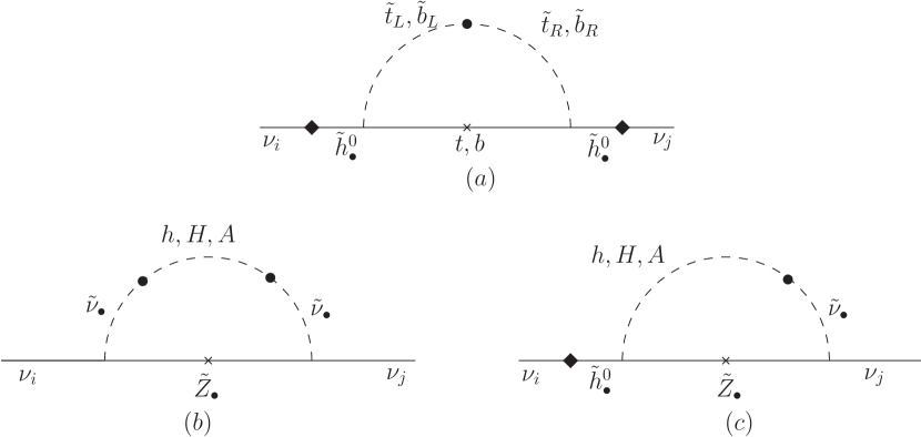
Figure 2: One-loop diagrams that contribute to the radiative masses for neutrinos. There is also an analogous diagram to (a) with a tau-stau loop in place of the quark-squark loop. As discussed in the text, the diagram with the top quark-squark loop in (a) only contributes to the mass of $\nu_{3}$ (the one neutrino massive at tree-level) but not to the masses of $\nu_{1}$ and $\nu_{2}$. The crosses denote fermion mass insertions and the solid circle denotes bilinear mixing between different scalars. The external neutrino lines with a diamond (and $\tilde{h}_{u}/\tilde{h}_{d}$ at the other end) symbolize that the neutrinos $\nu_{i}/\nu_{j}$ ($i,j=1,2,3$) couple to the quark-squark system via their $\tilde{h}_{u}/\tilde{h}_{d}$ content, and so the “internal higgsino line” is not a propagator in a Feynman diagram.

The order of magnitude of the contribution from Fig. 2a is given by,

$$m_{\nu}^{\rm rad}\sim\frac{3}{16\pi^{2}}Y_{q}^{2}m_{q}\sin 2\theta_{q}\ln\left(\frac{m_{\tilde{q}_{2}}^{2}}{m_{\tilde{q}_{1}}^{2}}\right)\frac{\epsilon^{2}}{m_{SUSY}^{2}},$$ (52)

where $q=t,b$, $Y_{q}$ is the quark Yukawa coupling, $\theta_{q}$ is the corresponding squark mixing angle, and $m_{\tilde{q}_{1,2}}$, the masses of the squarks. Detailed analyses bilinear ; valle of bilinear $R$-parity violation have shown that the radiatively generated neutrino mass is compatible with the solar neutrino mass scale $\Delta m^{2}_{\rm solar}=8\times 10^{-5}$ eV², obtained kamland by interpreting the deficit of solar neutrinos as oscillations between neutrinos with this smaller mass difference.

We now turn to contributions from the diagrams in Fig. 2b and Fig. 2c that have been examined in detail in Ref.Dav-Los ; Gros-Rak , where it has been shown that the contributions from the loops in diagrams b are generally larger than those from diagrams c. More importantly, a naive estimate of these contributions obtained using loop factors, coupling constant and mass insertions as we did for diagrams a gives a completely wrong answer because of large cancellations between contributions between the loop with $h,H$ and with $A$ that cause the total contribution to vanish, both in the (unphysical) limit where $m_{h}=m_{A}=m_{H}$, and in the decoupling limit where $m_{A},m_{H}\rightarrow\infty$, with $m_{h}$ and -ino masses fixed. The numerical analysis in Ref.Gros-Rak shows that this contribution, which scales as $1/\cos^{2}\beta$, is suppressed from its naive value by a factor of about $10^{-3}-10^{-2}$. For $\tan\beta$ in its intermediate range $\sim 30$ yields $m_{\nu}^{\rm rad}\sim 10^{-2}$ eV, in general agreement with the solar neutrino mass scale, for $b_{\epsilon}\sim(1-3)m_{\rm SUSY}\epsilon$.

We have thus seen that our model naturally yields the right scale of neutrino masses. A detailed analysis of neutrino masses and mixings, and comparison with the observed data is beyond the scope of this paper. Neutrino phenomenology for models with bilinear $R$-parity violation has been examined in detail in Ref.valle where it has been shown that it is possible to accommodate the pattern of neutrino masses together with the large mixing angles that provide a good fit to the solar and the atmospheric neutrino data. For the “minimal” boundary conditions used in this analysis, the potentially large contributions from diagrams in Fig. 2b and Fig. 2c appear to be subdominant. The analyses of Ref.adl illustrate that these contributions can, however, be dominant, and further that both a normal as well as an inverted hierarchy may be possible within this framework. We will refer the interested reader to these studies for details. Before moving on, we remind the reader that our model differs sharply from the $U(1)^{\prime}$ model of Ref. LMW in that we do not include independent right-handed neutrino fields.

IV.3 New Particles at the TeV scale: Masses and Decay patterns

We now focus our attention on the effective theory, valid at the TeV scale, that is relevant for phenomenological analyses of new physics signals at high energy colliders such as the LHC, or from various direct and indirect searches for dark matter that are very topical today. This theory is a softly broken supersymmetric $SU(3)_{C}\times SU(2)_{L}\times U(1)_{Y}$ gauge theory, with the particle content of the MSSM augmented, as we have already seen, by additional supermultiplets of exotic particles with properties that we discuss below. The underlying $U(1)^{\prime}$ gauge symmetry (which is spontaneously broken at the scale $\Lambda\sim 10^{11}$ GeV), restricts the forms of both the superpotential as well as of the SSB terms.

IV.3.1 MSSM superpartners

We have already seen that the non-trivial gauge kinetic function that we have introduced in (3) leads to weak scale masses for MSSM gauginos. Since there is no reason for the coefficients $f_{(\alpha)}$ to be the same, we will generically expect that these gaugino masses are not universal. Of course, embedding the model into a SUSY GUT framework may yield a common mass for the gauginos.

Although the $U(1)^{\prime}$ gauge boson, which acquires a mass by the Higgs mechanism, and the associated gaugino-higgsino states essentially decouple from TeV scale physics, the $U(1)^{\prime}$ leaves its imprint on the scalar spectrum via a contribution from the so-called $U(1)^{\prime}$ $D$-term contributions Dterm scalar SSB mass parameters. Thus the scalar mass parameters are given by,

$$m_{\bullet}^{2}=m_{\bullet}^{2}({\rm high})+{\cal Q}_{\bullet}\times D,$$ (53)

where $m_{\bullet}^{2}({\rm high})$ is the SSB scalar mass parameter (in general, non-universal if the non-minimal Kähler potential terms in (3) are significant) for the MSSM scalars induced by gravitational interactions, ${\cal Q}_{\bullet}$ is the $U(1)^{\prime}$ charge of the corresponding field as given in (46), and $D$ is a parameter (positive or negative) with dimension of mass squared, and a magnitude typically around the weak scale squared. In scenarios where the high scale SSB parameters are, for some reason, universal (remember that scalars of the first two generations with the same MSSM quantum numbers must be approximately degenerate for phenomenological reasons), the determination of scalar masses will provide information about the underlying $U(1)^{\prime}$ charges of MSSM fields. We remind the reader that $m_{H_{u}}^{2}<m_{H_{d}}^{2}$ facilitates radiative electroweak symmetry breaking.

The heavier MSSM superpartners decay as usual, mainly via their gauge and gaugino couplings, though effects of third generation Yukawa couplings may also be relevant BDT . An important difference from $R$-parity conserving models most extensively studied in the literature is that the would-be lightest supersymmetric particle (which, for defniteness, we will take to be the lightest neutralino, $\widetilde{Z}_{1}$) can decay via its neutrino component that is induced by the lepton-number-violating superpotential term. We may estimate this component to be ${\cal O}(\epsilon_{i}/\mu)\sim 10^{-7}$, which (very roughly speaking) gives a lifetime of $\stackrel{{\scriptstyle<}}{{\sim}}10^{-12}$ s [$10^{-8}$ s], assuming that the vector bosons in $\widetilde{Z}_{1}\rightarrow W^{\pm}\ell^{\mp}$ or $\widetilde{Z}_{1}\rightarrow Z\nu$ are real [virtual] neutra . Thus, except when the neutralino is lighter than $M_{W}$, we would expect it to decay within the detector with, or without, a discernable vertex separation.

IV.3.2 Exotics

In addition to the MSSM fields, we have seen that our model includes several TeV scale exotics. First, we have the coloured $K_{i}$, $K_{i}^{\prime}$ (both scalar and fermion) at the TeV scale, as we can see from the superpotential in (27), remembering that $\langle X_{1}\rangle=\Lambda$. Also, as we have seen in Table 1 the scalars $X_{l}$ and $X_{I}$ (and as can be seen from (27) also the fermions) acquire weak scale masses. These particles couple to SM particles only via the very suppressed $U(1)^{\prime}$ gauge interactions (or even more weakly, via gravity or via the Planck scale suppressed superpotential interactions), only the coloured $\hat{K}_{i}$ and $\hat{K}_{i}^{\prime}$ fields are of phenomenological interest exotic .

We first observe that with integer hypercharge assignment for $\hat{K}_{i}$ and $\hat{K}^{\prime}_{i}$, the lightest of the colour triplet states with each integer hypercharge, be it a boson or a fermion, will be stable since ordinary (s)quarks have fractional charges. For the fractional hypercharge case that we have considered, the lightest of the $K_{1}/K_{1}^{\prime}$ states is stable because the colour triplet state has charged $+\frac{1}{3}$, while the anti-triplet has the charged $-\frac{1}{3}$. Surprisingly, the lightest of the $K_{2,3}$ and $K_{2,3}^{\prime}$ states is also stable, despite the fact that $\hat{K}_{2,3}^{\prime}$ and $\hat{U}^{c}$ have the same $SU(3)_{C}\times SU(2)_{L}\times U(1)_{Y}$ quantum numbers, and so may be expected to mix upon $U(1)^{\prime}$ breaking via a term $\hat{U}^{c}\hat{K}_{2,3}$ that may be induced in the superpotential when $\hat{X}_{1,2}$ or $\hat{Y}_{1,2}$ acquire $vevs$. One can, however, readily check from the $U(1)^{\prime}$ charges in (46) that one would require fractional powers of $\hat{X}_{1,2}$ and/or $\hat{Y}_{1,2}\times\hat{U}^{c}\hat{K}_{2,3}$ in the superpotential to maintain the underlying $U(1)^{\prime}$ invariance. We thus conclude that such a mixing (that would have led to the decay of “the $K$ states”) is not allowed. A similar analysis shows that $\hat{K}_{2,3}^{\prime}\hat{D}^{c}\hat{D}^{c}$ term (which would allow the decays $K_{2,3}^{\prime}\rightarrow dd$, or $\tilde{K}_{2,3}\rightarrow d\tilde{d}_{R}^{(*)}$ or the conjugate modes) or the $\hat{H}_{u}\hat{Q}\hat{K}_{2,3}^{\prime}$ terms are also not allowed for the same set of values of $\frac{3{\cal Y}_{1}}{2{\cal X}_{1}}$ that we have examined.

Finally, we turn to the case where $y(\hat{K}_{i})=(-\frac{2}{3},\frac{4}{3},\frac{4}{3})$ that we considered at the end of Sec. III.2 so that the coloured exotics have the same MSSM charges as the singlet quark superfields. We have checked that even in this case mixing between $K_{1}$ scalars/fermions with singlet down squarks/quarks is forbidden because the $U(1)^{\prime}$ charge of $\hat{K}_{1}\hat{D}^{c}$ equals $\frac{277}{27}{\cal X}_{1}$. Mixing between $\hat{K}_{2,3}$ and $\hat{U}$ remains forbidden exactly as before since the corresponding $U(1)^{\prime}$ charges are unaffected by the flip of the weak hypercharge of $\hat{K}_{1}$. We have also checked that $U(1)^{\prime}$ breaking does not induce $\hat{H}_{d}\hat{Q}\hat{K}_{1}^{\prime}$, $\hat{Q}\hat{Q}\hat{K}_{1}$, $\hat{U}^{c}\hat{D}^{c}\hat{K}_{1}^{\prime}$, $\hat{U}^{c}\hat{E}^{c}\hat{K}_{1}$ and $\hat{L}\hat{Q}\hat{K}_{1}^{\prime}$ couplings since $U(1)^{\prime}$ invariance can only be maintained if these operators are multiplied by fractional powers of $\hat{X}_{1,2}$ and/or $\hat{Y}_{1,2}$ fields. This situation thus seems to be different from that in the models in Ref. ma2 , LMW and ma where couplings of the exotics to ordinary particles are possible when the exotics have the same weak hypercharges as the singlet quarks.

IV.4 Collider Signals

Since the $R$-parity violating couplings of MSSM superpartners are constrained by the observed neutrino masses to be rather small, these would dominantly be pair-produced at colliders via their gauge interactions, with cross sections as in the well-studied $R$-parity conserving models. They would then cascade decay casca to lighter sparticles as usual. The impact of the induced $R$-parity violating couplings is that the $\widetilde{Z}_{1}$ (which we have assumed to be the lightest MSSM superpartner) produced at the end of the cascade is itself unstable and decays via $\widetilde{Z}_{1}\rightarrow\ell W^{(*)}$ and $\widetilde{Z}_{1}\rightarrow\nu Z^{(*)}$ as discussed above. The (real or virtual) vector bosons decay to quarks and leptons with branching fractions given by the SM. In addition, the neutralino may decay via $\widetilde{Z}_{1}\rightarrow h\ ({\rm or}\ A,H)+\nu$, where $h$ dominantly decays via $b\bar{b}$. We refer the reader to Ref.neutra ; neutbf , where the branching fractions for the decay of the neutralino have been examined in detail. We only mention that while the $E_{T}^{\rm miss}$ signatures may be degraded in this $R$-parity violating scenario, the presence of charged leptons, $b$-quarks and potential vertex gaps provide additional handles for SUSY searches at colliders bkt ; neutbf ; neutra .

The stable coloured exotics that are necessary to cancel the $[SU(3)_{C}]^{2}\times U(1)^{\prime}$ anomaly will provide the smoking-gun signature of our scenario if they are accessible at the LHC, or at a future Very Large Hadron Collider. Once produced, the lighter of the colour triplet/anti-triplet $\hat{K}_{i}/\hat{K}_{i}^{\prime}$ scalar or fermion would pair up with an ordinary anti-quark/quark to form a heavy hadron, which then decays to the stable ground state of the exotic (s)quark–light antiquark system (or its conjugate). For the case of integrally charged $K$’s, as well as for the case where the colour-triplet $\hat{K}_{1}$ has the “wrong” sign of the weak hypercharge, this stable hadron will be fractionally charged, while in all other cases it will either be neutral or integrally charged. The penetrating track of a slow-moving, charged heavy particle provides a characteristic signature for the heavy charged hadron. Indeed, even in the case that the ground state is electrically neutral, charge exchange interactions of this hadron with the nucleon in a detector may transmute the neutral hadron to its charged isospin partner, resulting a sudden appearance of a track in the detector drees . Signals from stable quarks, squarks and gluino-hadrons in collider experiments have been examined in the literature drees ; stable . Experiments at the Fermilab Tevatron has carried out a search for penetrating tracks of slow-moving heavy particles and the non-observation of any signal has led to upper limits on the corresponding cross sections. These limits can then be translated to lower bounds on masses of various quasi-stable exotic particles: about 250 GeV for stable top-squarks and about 170/206 GeV for charged winos/higgsinos stable_tev . Even with a modest integrated luminosity of understood data, the claimed LHC reach for gluino-hadrons/top squarks exceeds 1600/800 GeV stable_lhc .

Before closing this section, we remark that, because the exotic particles have negligible couplings to SM particles, the low energy constraints on supersymmetry, e.g. from the branching ratios $b\rightarrow s\gamma$, $b\rightarrow s\ell\bar{\ell}$, $g_{\mu}-2$ etc. will be essentially as in the MSSM with the corresponding parameters.

IV.5 Cosmology and dark matter

In our scenario, we lose the neutralino as a thermal dark matter candidate since it decays via $R$-parity violating couplings that give rise to neutrino masses. While this may be viewed as a negative, it does not exclude the model, since dark matter may reside in different sector of the theory. Observation of a dark matter signal in direct searches for neutralinos would rule out our model. In this connection, we mention that it may be possible to modify the model to allow more than one pair of $SU(2)_{L}$ doublets ma with different $U(1)^{\prime}$ quantum numbers (which do not acquire a $vev$) such that a discrete subgroup under which the new doublet transforms non-trivially is left unbroken.

A potentially more serious problem is the presence of coloured TeV scale exotics in the $\hat{K}-\hat{K}^{\prime}$ sector. These would bind with ordinary nuclei to form exotic isotopes whose expected abundance (from thermal production in the Big Bang)wolfram exceeds by orders of magnitude the upper limitshemmick on the exotic isotope fraction for masses up to $\sim 10$ TeV: see Ref. glashow . These bounds may be evaded if the reheating temperature after inflation is smaller than the mass of the stable $K$-particles. While this is not currently fashionable, we are not aware of any considerations that exclude this possibility. Since the renormalizable baryon number violating operators have extremely small couplings in our framework, low scale baryogenesis mechanisms of Ref. baryogenesis do not apply , and we need to examine whether electroweak baryogenesis ewbar can be accommodated within the model.

V Summary

We have constructed a theoretically consistent and phenomenologically viable supergravity model where we impose only local symmetries to restrict the dynamics. We fix the SUSY breaking scale by hand to be $\Lambda\sim 10^{11}$ GeV, but otherwise assume that all new, i.e. non-SM, parameters are given by the natural values allowed by the underlying symmetries. Our gauge group is $SU(3)_{C}\times SU(2)_{L}\times U(1)_{Y}\times U(1)^{\prime}$, where the $U(1)^{\prime}$ gauge symmetry (which is spontaneously broken at the intermediate scale) plays multiple roles: it serves to solve the $\mu$ and $b_{\mu}$ problems, restricts the form of $R$-parity violating interactions so that dimension three and dimension four baryon number violating superpotential couplings, and in a class of models all $\Delta B=1$ couplings, are absent (solving the problem of proton lifetime in SUSY models), and determines the order of magnitude of the corresponding renormalizable lepton number violating interactions. Specifically, (in the superfield basis where the fermionic components are the $e,\mu$ and $\tau$ leptons along with the $h_{d}$ higgsino) trilinear lepton number violating couplings in the superpotential are negligible, so that “bilinear $R$-parity violation” dominates. This, in turn, allows us to obtain a novel connection between the scale of SUSY breaking and the mass scale of active neutrinos, that allows us to accommodate the observed pattern of neutrino mases and mixing angles.

The low energy theory at the (multi)-TeV scale is the MSSM augmented by several new fields. SUSY phenomenology would be largely that for models with bilinear $R$-parity violation, and has been examined in the literature. We must, however, keep in mind that often assumed scalar universality of the mSUGRA model would generically not apply here, and perhaps, even gaugino mass parameters may be non-universal. The only relevant effect of $R$-parity violation in collider experiments would be that the would-be LSP is unstable; its lepton daughters, and possible displaced vertex would provide additional handles to enhance the SUSY signal over SM background. Very low energy phenomenology (rare decays, $g_{\mu}-2$, $CP$ violation of SM particles) is unaltered from the MSSM because the new fields are extremely weakly coupled to SM particles.

There must, however, be new colour triplet, weak iso-singlet superfields with either the usual quark quantum numbers or exotic quantum numbers (integrally charged quarks, or charged +$\frac{1}{3}$ quarks) which would be copiously produced at a hadron collider if they are kinematically accessible. Quite possibly though these fields may be at the multi-TeV scale, and so would require a Very Large Hadron Collider for their experimental scrutiny. The unambiguious prediction of our model (which serves to distinguish it from other models with $U(1)$ gauge extensions) is that there are several stable coloured particles (whether these are fermions or scalars depends on details of parameters) which would combine with light quarks/antiquarks to form stable hadrons. Such hadrons would be readily discoverable at a high energy hadron collider, where it would even be possible to determine their mass.

Although these multi-TeV stable coloured particles provide the most striking phenomenological signature of our model, they also cause its demise if they are produced in the Big Bang, since their existence is excluded by very stringent upper limits on the abundance of heavy isotopes of hydrogen and other elements. We must, therefore assume that the reheating temperature after inflation was low enough not to produce these particles, and further, that the observed baryon asymmetry arises from sphaleron effects. Finally, we do not have a WIMP candidate for DM, so that detection of DM via direct searches would be a decisive blow to our model.

References

- (1) H. Baer and X. Tata, Weak Scale Supersymmetry: From Superfields to Scattering Events, (Cambridge University Press, 2006); M. Drees, R. Godbole and P. Roy, Theory and Phenomenology of Sparticles, (World Scientific, 2004); P. Bin etruy, Supersymmetry (Oxford University Press, 2006); S. P. Martin, hep-ph/9709356.
- (2) N. Sakai, Z. Phys. C 11, 153 (1981); S. Dimopoulos and H. Georgi, Nucl. Phys. B 193, 150 (1981); E. Witten, Nucl. Phys. B 188, 513 (1982); R. Kaul, Phys. Lett. B 109, 19 (1982).
- (3) U. Amaldi, W. de Boer and H. Furstenau, Phys. Lett. B 260, 447 (1991).
- (4) G. Jungman, M. Kamionkowski and K. Griest, Phys. Rep. 267, 195 (1996).
- (5) J.E. Kim and H.P. Nilles, Phys. Lett. B 138, 150 (1984); G.F. Giudice and A. Masiero, Phys. Lett. B 206, 480 (1988); J.E. Kim and H.P. Nilles, Phys. Lett. B 263, 79 (1991); E.J. Chun, J.E. Kim and H.P. Nilles, Nucl. Phys. B 370, 105 (1992); J.A. Casas and C. Muñoz, Phys. Lett. B 306, 288 (1993); G. Dvali, G.F. Giudice and A. Pomarol, Nucl. Phys. B 478, 31 (1996); D.E. Lopez-Fogliani and C. Muñoz, Phys. Rev. Lett. 97, 041801 (2006). L. Hall, Y. Nomura and A. Pierce, Phys. Lett. B 538, 359 (2002) have suggested that the symmetry that protects may be an -symmetry.
- (6) N. Sakai and T. Yanagida, Nucl. Phys. B 197, 533 (1982); S. Weinberg, Phys. Rev. D26, 287 (1982); S. Dimopoulos, S. Raby and F. Wilczek, Phys. Lett. B 112, 133 (1982).
- (7) Models without flavour problems generally fall into three categories: models where scalars with the same gauge quantum numbers are roughly degenerate, models where the matrices for fermions and corresponding sfermions are aligned, and models where scalars are very heavy.
- (8) S. Giddings and A. Strominger, Nucl. Phys. B 307, 854 (1988); S. Coleman, Nucl. Phys. B 310, 643 (1988); G. Gilbert, Nucl. Phys. B 328, 159 (1989).
- (9) A. Chamseddine, R. Arnowitt and P. Nath, Phys. Rev. Lett. 49, 970 (1982); R. Barbieri, S. Ferrara and C. Savoy, Phys. lett B 119, 343 (1982); N. Ohta, Prog. Theor. Phys. 70, 542 (1983); L. Hall, J. Lykken and S. Weinberg, Phys. Rev. D 27, 2359 (1983).
- (10) J. Polonyi, Hungary Central Research Institute report KFKI-77-93 (1977) (unpublished).
- (11) S. Dimopoulos and H. Georgi, Ref. hier ; N. Sakai, Ref. hier .
- (12) S. Soni and H.A. Weldon, Phys. Lett. B 126, 215 (1983).
- (13) H. Baer and X. Tata, Ref. susy-text
- (14) G.F. Giudice and A. Masiero, Ref. mupro .
- (15) J.E. Kim and H.P. Nilles, Ref. mupro ..
-
(16)
P. Fayet, Nucl. Phys. B 90, 104 (1975); Phys. Lett. B 69 489
(1977); ibid. B 76, 575 (1978);
C. Aulakh and R. Mohapatra, Phys. Lett. B 121, 127 (1983); L. Hall and M. Suzuki, Nucl. Phys. B 231, 419 (1984); I-Hsiu Lee, Nucl. Phys. B 246, 120 (1984); A. Santamaria and J. Valle, Phys. Lett. B 195, 423 (1987); S. Dimopoulos and L. Hall, Phys. Lett. B 207, 210 (1987); R. Godbole et al. Nucl. Phys. B 401, 67 (1993); M. Hirsch et al. Phys. Rev. D 62, 113008 (2000). - (17) S. Weinberg, Ref.prodecay ; H.C. Cheng, B.A. Dobrescu and K.T. Matchev, Phys. Lett. B 439, 301 (1998); Nucl. Phys. B 543, 47 (1999); J. Erler, Nucl. Phys. B 586, 73 (2000); M. Aoki and N. Oshimo, Phys. Rev. Lett. 84, 5269 (2000); Phys. Rev. D 62, 055013 (2000);
- (18) E. Ma, Phys. Rev. Lett. 89, 041801 (2002).
- (19) K. Dienes, C. Kolda and J. March-Russel, Nucl. Phys. B 492, 104 (1997).
- (20) K. Kobayashi et al. (SuperKamiokande Collaboration) Phys. Rev. D 72, 052007 (2005).
- (21) L. Ibañez and G. G. Ross, Nucl. Phys. B 368, 3 (1992).
- (22) D. Castaño and S. Martin, Phys. Lett. B 340, 67 (1994); H. S. Lee, C. Luhn and K. Matchev, J. High Energy Phys. 0807, 065 (2008).
- (23) See, e.g. M. Hirsch and J.W.F. Valle, New J. Phys. 6, 76 (2004), and references therein.
- (24) Y. Fukuda et al. (Super-Kamiokande Collaboration) Phys. Rev. Lett 81, 1562 (1998).
- (25) For a review, see e.g. S. Hannestad, arXiv:hep-ph/041218 (2008), Table 2, and references cited therein. See also, E. Komatsu et al. arXiv:0803.0547 [astro-ph] (2008) for an update.
- (26) S. Abe et al. (Kamland Collaboration) Phys. Rev. Lett. 100, 221803 (2008).
- (27) S. Davidson and M. Losada, J. High Energy Phys. 05, 021 (2000); Phys. Rev. D 65, 075025 (2002).
- (28) Y. Grossman and S. Rakshit, Phys. Rev. D 69, 093002 (2004).
- (29) M.A. Diaz, M. Hirsch, W. Porod, J.C. Romao and J.W.F. Valle, Phys. Rev. D 68, 013009 (2003); see also Ref. bilinear .
- (30) A. Abada, S. Davidson and M. Losada, Phys. Rev. D 65, 075010 (2002); A. Abada, G. Bhattacharya and M. Losada, Phys. Rev. D 66, 071701 (2002).
- (31) H.S. Lee, K.T. Matchev and T.T. Wang, Phys. Rev. D 77, 015016 (2008).
- (32) M. Drees, Phys. Lett. B 181, 279 (1986); J. Hagelin and S. Kelley, Nucl. Phys. B 342, 95 (1990); A. Faraggi et al. Phys. Rev. D 45, 3272 (1992); Y. Kawamura and M. Tanaka, Prog. Theor. Phys. 91, 949 (1994); N. Polansky and A. Pomarol, Phys. Rev. D 51, 6532 (1995); H. C. Cheng and L. Hall, Phys. Rev. D 51, 5289 (1995); C. Kolda and S. Martin, Phys. Rev. D 53, 3871 (1993).
- (33) H. Baer, C. H. Chen, M. Drees, F. Paige and X. Tata, Phys. Rev. Lett. 79 986 (1997) and 80, 642 (1998) (E); H. Baer, C. H. Chen, M. Drees, F. Paige and X. Tata, Phys. Rev. D 58, 075008 (1998); ibid 59, 055014 (1999).
- (34) B. Mukhopadhyaya, S. Roy and F. Vissani, Phys. Lett. B 443, 191 (1998); S. Y. Choi, E. J. Chun, S. K. Kang, and J. S. Lee, Phys. Rev. D 60, 075002 (1999); W. Porod, M. Hirsch, J. Romao and J.W.F. Valle Phys. Rev. D 63, 115004 (2001).
- (35) For a recent study of isosinglet (s)quark phenomenology, see J. Kang, P. Langacker and B.D. Nelson, Phys. Rev. D 77, 035003 (2008).
- (36) E. Ma, Phys. Lett. B 659, 885 (2008); Mod. Phys. Lett. A 23, 721 (2008).
- (37) H. Baer, J. Ellis, G. Gelmini, D. V. Nanopoulos and X. Tata, Phys. Lett B 161, 175 (1985); G. Gamberini, Z. Physik C 30, 605 (1986); H. Baer, V. Barger, D. Karatas and X. Tata, Phys. Rev. D 36, 96, (1987); H. Baer, X. Tata and J. Woodside, Phys. Rev. D 45, 142 (1992).
- (38) A. Bartl et al. Nucl. Phys. B 600, 39 (2001); E. J. Chun, D. W. Jung, S. K. Kang, J. D. Park, Phys. Rev. D 66, 073003 (2002); F. de Campos et al., arXiv:0712.2156 (2007); M. Hirsch, A. Vicente and W. Porod, Phys. Rev. D 77, 075005 (2008). See also, P. Ghosh and S. Roy, arXiv:0812.0084 (2008), for a phenomenological discussion in the context of a qualitatively different model where both and the bilinear superpotential terms arise from s of a singlet sneutrino field.
- (39) H. Baer, C. Kao and X. Tata, Phys. Rev. D51, 2180 (1995); for the extent to which the LHC reach is degraded if the neutralino decays hadronically see, H. Baer, C. Chen and X. Tata, Phys. Rev. D 55, 1466 (1997).
- (40) M. Drees and X. Tata, Phys. Lett B 252, 695 (1990).
- (41) H. Baer, K. Cheung and J. Gunion, Phys. Rev. D59, 075002 (1999); M. Fairbairn et al. Phys. Rep. 438, 1 (2007) and refereinces therein.
- (42) D. Acosta et al. Phys. Rev. Lett. 90, 131801 (2003), and CDF-note 8701 (2005); For searches for stable non-strongly interacting charged particles, see V. M. Abazov et al. arXiv:0809.4472 [hep-ex].
- (43) S. Giagu, ATL-PHYS-PROC-2008-029 (2008). See also, M. Johannsen, Acta Physica Polonica, 38, 591 (2007).
- (44) S. Wolfram, Phys. Lett. B 82, 65 (1979); C.B. Dover, T. Gaisser and G. Steigman, Phys. Rev. Lett. 42, 1117 (1979).
- (45) T. Hemmick et. al., Phys. Rev. D 41, 2074 (1990).
- (46) A. de Rujula, S. Glashow and U. Sarid, Nucl. Phys. B 333, 173 (1990).
- (47) S. Dimopoulos and L. Hall, Phys. Lett. B 196, 135 (1987); J. Cline and S. Raby, Phys. Rev. D 43, 1781 (1991); K. Babu, R. Mohapatra, and S. Nasri, Phys. Rev. Lett. 97, 131301 (2006).
- (48) M. Carena, M. Quiros, A. Riotto A. Vilja and C. Wagner, Nucl. Phys. B 503, 387 (1997); C. Balázs et al. Phys. Rev. D 71, 075002 (2005) and references therein; T. Konstandin, T. Prokopec, M. Schmidt and M. Seco, Nucl. Phys. B 738, 1 (2006); D. Chung et al. arXiv: 0808.1144 [hep-ph] (2008).