Experimental investigation of nodal domains in the chaotic microwave rough billiard

Abstract

We present the results of experimental study of nodal domains of wave functions (electric field distributions) lying in the regime of Shnirelman ergodicity in the chaotic half-circular microwave rough billiard. Nodal domains are regions where a wave function has a definite sign. The wave functions $\Psi_{N}$ of the rough billiard were measured up to the level number $N=435$. In this way the dependence of the number of nodal domains $\aleph_{N}$ on the level number $N$ was found. We show that in the limit $N\rightarrow\infty$ a least squares fit of the experimental data reveals the asymptotic number of nodal domains $\aleph_{N}/N\simeq 0.058\pm 0.006$ that is close to the theoretical prediction $\aleph_{N}/N\simeq 0.062$. We also found that the distributions of the areas $s$ of nodal domains and their perimeters $l$ have power behaviors $n_{s}\propto s^{-\tau}$ and $n_{l}\propto l^{-\tau^{\prime}}$, where scaling exponents are equal to $\tau=1.99\pm 0.14$ and $\tau^{\prime}=2.13\pm 0.23$, respectively. These results are in a good agreement with the predictions of percolation theory. Finally, we demonstrate that for higher level numbers $N\simeq 220-435$ the signed area distribution oscillates around the theoretical limit $\Sigma_{A}\simeq 0.0386N^{-1}$.

In recent papers Blum et al. Blum2002 and Bogomolny and Schmit Bogomolny2002 have considered the distribution of the nodal domains of real wave functions $\Psi(x,y)$ in 2D quantum systems (billiards). The condition $\Psi(x,y)=0$ determines a set of nodal lines which separate regions (nodal domains) where a wave function $\Psi(x,y)$ has opposite signs. Blum et al. Blum2002 have shown that the distributions of the number of nodal domains can be used to distinguish between systems with integrable and chaotic underlying classical dynamics. In this way they provided a new criterion of quantum chaos, which is not directly related to spectral statistics. Bogomolny and Schmit Bogomolny2002 have shown that the distribution of nodal domains for quantum wave functions of chaotic systems is universal. In order to prove it they have proposed a very fruitful, percolationlike, model for description of properties of the nodal domains of generic chaotic system. In particular, the model predicts that the distribution of the areas $s$ of nodal domains should have power behavior $n_{s}\propto s^{-\tau}$, where $\tau=187/91$ Ziff1986 .

In this paper we present the first experimental investigation of nodal domains of wave functions of the chaotic microwave rough billiard. We tested experimentally some of important findings of papers by Blum et al. Blum2002 and Bogomolny and Schmit Bogomolny2002 such as the signed area distribution $\Sigma_{A}$ or the dependence of the number of nodal domains $\aleph_{N}$ on the level number $N$. Additionally, we checked the power dependence of nodal domain perimeters $l$, $n_{l}\propto l^{-\tau^{\prime}}$, where according to percolation theory the scaling exponent $\tau^{\prime}=15/7$ Ziff1986 , which was not considered in the above papers.

In the experiment we used the thin (height $h=8$ mm) aluminium cavity in the shape of a rough half-circle (Fig. 1). The microwave cavity simulates the rough quantum billiard due to the equivalence between the Schrödinger equation and the Helmholtz equation Hans ; Hans2 . This equivalence remains valid for frequencies less than the cut-off frequency $\nu_{c}=c/2h\simeq 18.7$ GHz, where c is the speed of light. The cavity sidewalls are made of 2 segments. The rough segment 1 is described by the radius function $R(\theta)=R_{0}+\sum_{m=2}^{M}{a_{m}\sin(m\theta+\phi_{m})}$, where the mean radius $R_{0}$=20.0 cm, $M=20$, $a_{m}$ and $\phi_{m}$ are uniformly distributed on [0.269,0.297] cm and [0,2$\pi$], respectively, and $0\leq\theta<{\pi}$. It is worth noting that following our earlier experience Hlushchuk01b ; Hlushchuk01 we decided to use a rough half-circular cavity instead of a rough circular cavity because in this way we avoided nearly degenerate low-level eigenvalues, which could not be possible distinguished in the measurements. As we will see below, a half-circular geometry of the cavity was also very suitable in the accurate measurements of the electric field distributions inside the billiard.

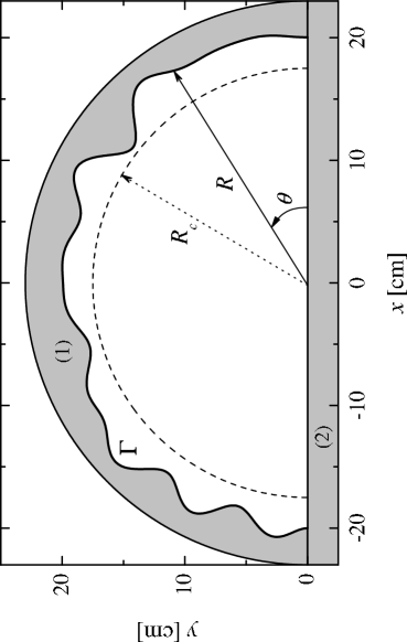
Figure 1: Sketch of the chaotic half-circular microwave rough billiard in the $xy$ plane. Dimensions are given in cm. The cavity sidewalls are marked by 1 and 2 (see text). Squared wave functions $|\Psi_{N}(R_{c},\theta)|^{2}$ were evaluated on a half-circle of fixed radius $R_{c}=17.5$ cm. Billiard’s rough boundary $\Gamma$ is marked with the bold line.

The surface roughness of a billiard is characterized by the function $k(\theta)=(dR/d\theta)/R_{0}$. Thus for our billiard we have the angle average $\tilde{k}=(\left<k^{2}(\theta)\right>_{\theta})^{1/2}\simeq 0.488$. In such a billiard the dynamics is diffusive in orbital momentum due to collisions with the rough boundary because $\tilde{k}$ is much above the chaos border $k_{c}=M^{-5/2}=0.00056$ Frahm97 . The roughness parameter $\tilde{k}$ determines also other properties of the billiard Frahm . The eigenstates are localized for the level number $N<N_{e}=1/128\tilde{k}^{4}$. Because of a large value of the roughness parameter $\tilde{k}$ the localization border lies very low, $N_{e}\simeq 1$. The border of Breit-Wigner regime is $N_{W}=M^{2}/48\tilde{k}^{2}\simeq 35$. It means that between $N_{e}<N<N_{W}$ Wigner ergodicity Frahm ought to be observed and for $N>N_{W}$ Shnirelman ergodicity should emerge. In 1974 Shnirelman Shnirelman proved that quantum states in chaotic billiards become ergodic for sufficiently high level numbers. This means that for high level numbers wave functions have to be uniformly spread out in the billiards. Frahm and Shepelyansky Frahm showed that in the rough billiards the transition from the exponentially localized states to the ergodic ones is more complicated and can pass through an intermediate regime of Wigner ergodicity. In this regime the wave functions are nonergodic and compose of rare strong peaks distributed over the whole energy surface. In the regime of Shnirelman ergodicity the wave functions should be distributed homogeneously on the energy surface.

In this paper we focus our attention on Shnirelman ergodicity regime.

One should mention that rough billiards and related systems are of considerable interest elsewhere, e.g. in the context of dynamic localization Sirko00 , localization in discontinuous quantum systems Borgonovi , microdisc lasers Yamamoto ; Stone and ballistic electron transport in microstructures Blanter .

In order to investigate properties of nodal domains knowledge of wave functions (electric field distributions inside the microwave billiard) is indispensable. To measure the wave functions we used a new, very effective method described in Savytskyy2003 . It is based on the perturbation technique and preparation of the “trial functions”. Below we will describe shortly this method.

The wave functions $\Psi_{N}(r,\theta)$ (electric field distribution $E_{N}(r,\theta)$ inside the cavity) can be determined from the form of electric field $E_{N}(R_{c},\theta)$ evaluated on a half-circle of fixed radius $R_{c}$ (see Fig. 1). The first step in evaluation of $E_{N}(R_{c},\theta)$ is measurement of $|E_{N}(R_{c},\theta)|^{2}$. The perturbation technique developed in Slater52 and used successfully in Slater52 ; Sridhar91 ; Richter00 ; Anlage98 was implemented for this purpose. In this method a small perturber is introduced inside the cavity to alter its resonant frequency according to

$$\nu-\nu_{N}=\nu_{N}(aB_{N}^{2}-bE_{N}^{2}),$$

where $\nu_{N}$ is the $N$th resonant frequency of the unperturbed cavity, $a$ and $b$ are geometrical factors. Equation (1) shows that the formula can not be used to evaluate $E_{N}^{2}$ until the term containing magnetic field $B_{N}$ vanishes. To minimize the influence of $B_{N}$ on the frequency shift $\nu-\nu_{N}$ a small piece of a metallic pin (3.0 mm in length and 0.25 mm in diameter) was used as a perturber. The perturber was moved by the stepper motor via the Kevlar line hidden in the groove (0.4 mm wide, 1.0 mm deep) made in the cavity’s bottom wall along the half-circle $R_{c}$. Using such a perturber we had no positive frequency shifts that would exceed the uncertainty of frequency shift measurements (15 kHz). We checked that the presence of the narrow groove in the bottom wall of the cavity caused only very small changes $\delta\nu_{N}$ of the eigenfrequencies $\nu_{N}$ of the cavity $|\delta\nu_{N}|/\nu_{N}\leq 10^{-4}$. Therefore, its influence into the structure of the cavity’s wave functions was also negligible. A big advantage of using hidden in the groove line was connected with the fact that the attached to the line perturber was always vertically positioned what is crucial in the measurements of the square of electric field $E_{N}$. To eliminate the variation of resonant frequency connected with the thermal expansion of the aluminium cavity the temperature of the cavity was stabilized with the accuracy of 0.05 $\deg$.

Figure 2: Panel (a): Squared wave function $|\Psi_{435}(R_{c},\theta)|^{2}$ (in arbitrary units) measured on a half-circle with radius $R_{c}=17.5$ cm ($\nu_{435}\simeq 14.44$ GHz). Panel (b): The “trial wave function” $\Psi_{435}(R_{c},\theta)$ (in arbitrary units) with the correctly assigned signs, which was used in the reconstruction of the wave function $\Psi_{435}(r,\theta)$ of the billiard (see Fig. 3).

The regime of Shnirelman ergodicity for the experimental rough billiard is defined for $N>35$. Using a field perturbation technique we measured squared wave functions $|\Psi_{N}(R_{c},\theta)|^{2}$ for 156 modes within the region $80\leq N\leq 435$. The range of corresponding eigenfrequencies was from $\nu_{80}\simeq 6.44$ GHz to $\nu_{435}\simeq 14.44$ GHz. The measurements were performed at 0.36 mm steps along a half-circle with fixed radius $R_{c}=17.5$ cm. This step was small enough to reveal in details the space structure of high-lying levels. In Fig. 2 (a) we show the example of the squared wave function $|\Psi_{N}(R_{c},\theta)|^{2}$ evaluated for the level number $N=435$. The perturbation method used in our measurements allows us to extract information about the wave function amplitude $|\Psi_{N}(R_{c},\theta)|$ at any given point of the cavity but it doesn’t allow to determine the sign of $\Psi_{N}(R_{c},\theta)$ Stein95 . Our results presented in Savytskyy2003 suggest the following sign-assignment strategy: We begin with the identification of all close to zero minima of $|\Psi_{N}(R_{c},\theta)|$. Then the sign “minus” maybe arbitrarily assigned to the region between the first and the second minimum, “plus” to the region between the second minimum and the third one, the next “minus” to the next region between consecutive minima and so on. In this way we construct our “trial wave function” $\Psi_{N}(R_{c},\theta)$. If the assignment of the signs is correct we should reconstruct the wave function $\Psi_{N}(r,\theta)$ inside the billiard with the boundary condition $\Psi_{N}(r_{\Gamma},\theta_{\Gamma})=0$.

The wave functions of a rough half-circular billiard may be expanded in terms of circular waves (here only odd states in expansion are considered)

$$\Psi_{N}(r,\theta)=\sum_{s=1}^{L}a_{s}C_{s}J_{s}(k_{N}r)\sin(s\theta),$$

where $C_{s}=(\frac{\pi}{2}\int_{0}^{r_{max}}|J_{s}(k_{N}r)|^{2}rdr)^{-1/2}$ and $k_{N}=2\pi\nu_{N}/c$.

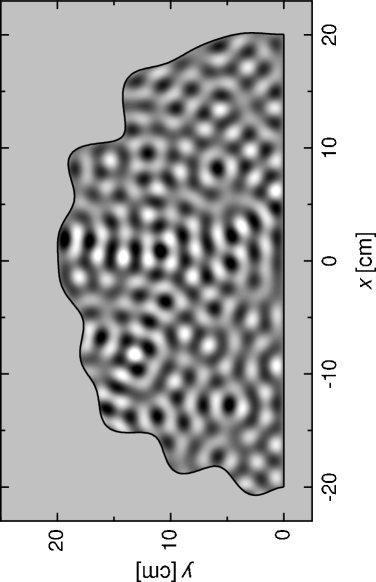
Figure 3: The reconstructed wave function $\Psi_{435}(r,\theta)$ of the chaotic half-circular microwave rough billiard. The amplitudes have been converted into a grey scale with white corresponding to large positive and black corresponding to large negative values, respectively. Dimensions of the billiard are given in cm.

In Eq. (2) the number of basis functions is limited to $L=k_{N}r_{max}=l_{N}^{max}$, where $r_{max}=21.4$ cm is the maximum radius of the cavity. $l_{N}^{max}=k_{N}r_{max}$ is a semiclassical estimate for the maximum possible angular momentum for a given $k_{N}$. Circular waves with angular momentum $s>L$ correspond to evanescent waves and can be neglected. Coefficients $a_{s}$ may be extracted from the “trial wave function” $\Psi_{N}(R_{c},\theta)$ via

$$a_{s}=[\frac{\pi}{2}C_{s}J_{s}(k_{N}R_{c})]^{-1}\int_{0}^{\pi}\Psi_{N}(R_{c},\theta)\sin(s\theta)d\theta.$$

Since our “trial wave function” $\Psi_{N}(R_{c},\theta)$ is only defined on a half-circle of fixed radius $R_{c}$ and is not normalized we imposed normalization of the coefficients $a_{s}$: $\sum_{s=1}^{L}|a_{s}|^{2}=1$. Now, the coefficients $a_{s}$ and Eq. (2) can be used to reconstruct the wave function $\Psi_{N}(r,\theta)$ of the billiard. Due to experimental uncertainties and the finite step size in the measurements of $|\Psi_{N}(R_{c},\theta)|^{2}$ the wave functions $\Psi_{N}(r,\theta)$ are not exactly zero at the boundary $\Gamma$. As the quantitative measure of the sign assignment quality we chose the integral $\gamma\int_{\Gamma}|\Psi_{N}(r,\theta)|^{2}dl$ calculated along the billiard’s rough boundary $\Gamma$, where $\gamma$ is length of $\Gamma$. In Fig. 2 (b) we show the “trial wave function” $\Psi_{435}(R_{c},\theta)$ with the correctly assigned signs, which was used in the reconstruction of the wave function $\Psi_{435}(r,\theta)$ of the billiard (see Fig. 3). Using the method of the “trial wave function” we were able to reconstruct 138 experimental wave functions of the rough half-circular billiard with the level number $N$ between 80 and 248 and 18 wave functions with $N$ between 250 and 435. The wave functions were reconstructed on points of a square grid of side $4.3\cdot 10^{-4}$ m. The remaining wave functions from the range $N=80-435$ were not reconstructed because of the accidental near-degeneration of the neighboring states or due to the problems with the measurements of $|\Psi_{N}(R_{c},\theta)|^{2}$ along a half-circle coinciding for its significant part with one of the nodal lines of $\Psi_{N}(r,\theta)$. These problems are getting much more severe for $N>250$. Furthermore, the computation time $t_{r}$ required for reconstruction of the ”trial wave function” scales like $t_{r}\propto 2^{n_{z}-2}$, where $n_{z}$ is the number of identified zeros in the measured function $|\Psi_{N}(R_{c},\theta)|$. For higher $N$, the computation time $t_{r}$ on a standard personal computer with the processor AMD Athlon XP 1800+ often exceeds several hours, what significantly slows down the reconstruction procedure.

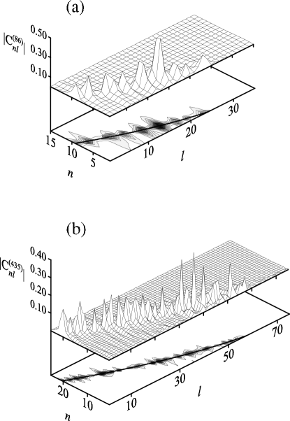
Figure 4: Structure of the energy surface in the regime of Shnirelman ergodicity. Here we show the moduli of amplitudes $|C^{(N)}_{nl}|$ for the wave functions: (a) $N=86$, (b) $N=435$. The wave functions are delocalized in the $n,l$ basis. Full lines show the semiclassical estimation of the energy surface (see text).

Ergodicity of the billiard’s wave functions can be checked by finding the structure of the energy surface Frahm97 . For this reason we extracted wave function amplitudes $C^{(N)}_{nl}=\left<n,l|N\right>$ in the basis $n,l$ of a half-circular billiard with radius $r_{max}$, where $n=1,2,3\ldots$ enumerates the zeros of the Bessel functions and $l=1,2,3\ldots$ is the angular quantum number. The moduli of amplitudes $|C^{(N)}_{nl}|$ and their projections into the energy surface for the representative experimental wave functions $N=86$ and $N=435$ are shown in Fig. 4. As expected, in the regime of Shnirelman ergodicity the wave functions are extended homogeneously over the whole energy surface Hlushchuk01 . The full lines on the projection planes in Fig. 4(a) and Fig. 4(b) mark the energy surface of a half-circular billiard $H(n,l)=E_{N}=k^{2}_{N}$ estimated from the semiclassical formula Hlushchuk01b : $\sqrt{(l^{max}_{N})^{2}-l^{2}}-l\arctan(l^{-1}\sqrt{(l^{max}_{N})^{2}-l^{2}})+\pi/4=\pi n$. The peaks $|C^{(N)}_{nl}|$ are spread almost perfectly along the lines marking the energy surface.

Figure 5: Amplitude distribution $P(\Psi A^{1/2})$ for the eigenstates: (a) $N=86$ and (b) $N=435$ constructed as histograms with bin equal to 0.2. The width of the distribution $P(\Psi)$ was rescaled to unity by multiplying normalized to unity wave function by the factor $A^{1/2}$, where $A$ denotes billiard’s area. Full line shows standard normalized Gaussian prediction $P_{0}(\Psi A^{1/2})=(1/\sqrt{2\pi})e^{-\Psi^{2}A/2}$.

An additional confirmation of ergodic behavior of the measured wave functions can be also sought in the form of the amplitude distribution $P(\Psi)$ Berry77 ; Kaufman88 . For irregular, chaotic states the probability of finding the value $\Psi$ at any point inside the billiard, without knowledge of the surrounding values, should be distributed as a Gaussian, $P(\Psi)\sim e^{-\beta\Psi^{2}}$. It is worth noting that in the above case the spatial intensity should be distributed according to Porter-Thomas statistics Hans2 . The amplitude distributions $P(\Psi A^{1/2})$ for the wave functions $N=86$ and $N=435$ are shown in Fig. 5. They were constructed as normalized to unity histograms with the bin equal to 0.2. The width of the amplitude distributions $P(\Psi)$ was rescaled to unity by multiplying normalized to unity wave functions by the factor $A^{1/2}$, where $A$ denotes billiard’s area (see formula (23) in Kaufman88 ). For all measured wave functions in the regime of Shnirelman ergodicity there is a good agreement with the standard normalized Gaussian prediction $P_{0}(\Psi A^{1/2})=(1/\sqrt{2\pi})e^{-\Psi^{2}A/2}$.

Figure 6: The number of nodal domains $\aleph_{N}$ (full circles) for the chaotic half-circular microwave rough billiard. Full line shows a least squares fit $\aleph_{N}=a_{1}N+b_{1}\sqrt{N}$ to the experimental data (see text), where $a_{1}=0.058\pm 0.006$, $b_{1}=1.075\pm 0.088$. The prediction of the theory of Bogomolny and Schmit Bogomolny2002 $a_{1}=0.062$.

The number of nodal domains $\aleph_{N}$ vs. the level number $N$ in the chaotic microwave rough billiard is plotted in Fig. 6. The full line in Fig. 6 shows a least squares fit $\aleph_{N}=a_{1}N+b_{1}\sqrt{N}$ of the experimental data, where $a_{1}=0.058\pm 0.006$, $b_{1}=1.075\pm 0.088$. The coefficient $a_{1}=0.058\pm 0.006$ coincides with the prediction of the percolation model of Bogomolny and Schmit Bogomolny2002 $\aleph_{N}/N\simeq 0.062$ within the error limits. The second term in a least squares fit corresponds to a contribution of boundary domains, i.e. domains, which include the billiard boundary. Numerical calculations of Blum et al. Blum2002 performed for the Sinai and stadium billiards showed that the number of boundary domains scales as the number of the boundary intersections, that is as $\sqrt{N}$. Our results clearly suggest that in the rough billiard, at low level number $N$, the boundary domains also significantly influence the scaling of the number of nodal domains $\aleph_{N}$, leading to the departure from the predicted scaling $\aleph_{N}\sim N$.

Figure 7: Distribution of nodal domain areas. Full line shows the prediction of percolation theory $\log_{10}(\langle n_{s}/n\rangle)=-\frac{187}{91}\log_{10}(\langle s/s_{min}\rangle)$. A least squares fit $\log_{10}(\langle n_{s}/n\rangle)=a_{2}-\tau\log_{10}(\langle s/s_{min}\rangle)$ of the experimental results lying within the vertical lines yields the scaling exponent $\tau=1.99\pm 0.14$ and $a_{2}=-0.05\pm 0.04$. The result of the fit is shown by the dashed line.

The bond percolation model Bogomolny2002 at the critical point $p_{c}=1/2$ allows us to apply other results of percolation theory to the description of nodal domains of chaotic billiards. In particular, percolation theory predicts that the distributions of the areas $s$ and the perimeters $l$ of nodal clusters should obey the scaling behaviors: $n_{s}\propto s^{-\tau}$ and $n_{l}\propto l^{-\tau^{\prime}}$, respectively. The scaling exponents Ziff1986 are found to be $\tau=187/91$ and $\tau^{\prime}=15/7$. In Fig. 7 we present in logarithmic scales nodal domain areas distribution $\langle n_{s}/n\rangle$ vs. $\langle s/s_{min}\rangle$ obtained for the microwave rough billiard. The distribution $\langle n_{s}/n\rangle$ was constructed as normalized to unity histogram with the bin equal to 1. The areas $s$ of nodal domains were calculated by summing up the areas of the nearest neighboring grid sites having the same sign of the wave function. In Fig. 7 the vertical axis $\langle n_{s}/n\rangle=\frac{1}{N_{T}}\sum_{i=1}^{N_{T}}n_{s}^{(N)}/n^{(N)}$ represents the number of nodal domains $n_{s}^{(N)}$ of size $s$ divided by the total number of domains $n^{(N)}$ averaged over $N_{T}=18$ wave functions measured in the range $250\leq N\leq 435$. In these calculations we used only the highest measured wave functions in order to minimize the influence of boundary domains on nodal domain areas distribution. Following Bogomolny and Schmit Bogomolny2002 , the horizontal axis is expressed in the units of the smallest possible area $s_{min}^{(N)}$, $\langle s/s_{min}\rangle=\frac{1}{N_{T}}\sum_{i=1}^{N_{T}}s/s_{min}^{(N)}$, where $s_{min}^{(N)}=\pi(j_{01}/k_{N})^{2}$ and $j_{01}\simeq 2.4048$ is the first zero of the Bessel function $J_{0}(j_{01})=0$. The full line in Fig. 7 shows the prediction of percolation theory $\log_{10}(\langle n_{s}/n\rangle)=-\frac{187}{91}\log_{10}(\langle s/s_{min}\rangle)$. In a broad range of $\log_{10}(\langle s/s_{min}\rangle)$, approximately from 0.2 to 1.3, which is marked by the two vertical lines the experimental results follow closely the theoretical prediction. Indeed, a least squares fit $\log_{10}(\langle n_{s}/n\rangle)=a_{2}-\tau\log_{10}(\langle s/s_{min}\rangle)$ of the experimental results lying within the vertical lines yields the scaling exponent $\tau=1.99\pm 0.14$ and $a_{2}=-0.05\pm 0.04$, which is in a good agreement with the predicted $\tau=187/91\simeq 2.05$. The dashed line in Fig. 7 shows the results of the fit. In the vicinity of $\log_{10}(\langle s/s_{min}\rangle)\simeq 1$ and $1.2$ small excesses of large areas are visible. A similar situation, but for larger $\log_{10}(s/s_{min})>4$, can be also observed in the nodal domain areas distribution presented in Fig. 5 in Ref. Bogomolny2002 for the random wave model. The exact cause of this behavior is not known but we can possible link it with the limited number of wave functions used for the preparation of the distribution.

Figure 8: Distribution of nodal domain perimeters. Full line shows the prediction of percolation theory $\log_{10}(\langle n_{l}/n\rangle)=-\frac{15}{7}\log_{10}(\langle l/l_{min}\rangle)$. A least squares fit $\log_{10}(\langle n_{l}/n\rangle)=a_{3}-\tau^{\prime}\log_{10}(\langle l/l_{min}\rangle)$ of the experimental results lying within the range marked by the vertical lines yields $\tau^{\prime}=2.13\pm 0.23$ and $a_{3}=0.04\pm 0.21$. The result of the fit is shown by the dashed line.

Nodal domain perimeters distribution $\langle n_{l}/n\rangle$ vs. $\langle l/l_{min}\rangle$ is shown in logarithmic scales in Fig. 8. The distribution $\langle n_{l}/n\rangle$ was constructed as normalized to unity histogram with the bin equal to 1 . The perimeters of nodal domains $l$ were calculated by identifying the continues paths of grid sites at the domains boundaries. The averaged values $\langle n_{l}/n\rangle$ and $\langle l/l_{min}\rangle$ are defined similarly as previously defined $\langle n_{s}/n\rangle$ and $\langle s/s_{min}\rangle$, e.g. $\langle l/l_{min}\rangle=\frac{1}{N_{T}}\sum_{i=1}^{N_{T}}l/l_{min}^{(N)}$, where $l_{min}^{(N)}=2\pi\sqrt{s_{min}^{(N)}/\pi}=2\pi(j_{01}/k_{N})$ is the perimeter of the circle with the smallest possible area $s_{min}^{(N)}$. The full line in Fig. 8 shows the prediction of percolation theory $\log_{10}(\langle n_{l}/n\rangle)=-\frac{15}{7}\log_{10}(\langle l/l_{min}\rangle)$. Also in this case the agreement between the experimental results and the theory is good what is well seen in the range $0.2<\log_{10}(\langle l/l_{min}\rangle)<1.2$, which is marked by the two vertical lines. A least squares fit $\log_{10}(\langle n_{l}/n\rangle)=a_{3}-\tau^{\prime}\log_{10}(\langle l/l_{min}\rangle)$ of the experimental results lying within the marked range yields $\tau^{\prime}=2.13\pm 0.23$ and $a_{3}=0.04\pm 0.21$. The result of the fit is shown in Fig. 8 by the dashed line. As we see the scaling exponent $\tau^{\prime}=2.13\pm 0.23$ is close to the exponent predicted by percolation theory $\tau^{\prime}=15/7\simeq 2.14$. The above results clearly demonstrate that percolation theory is very useful in description of the properties of wave functions of chaotic billiards.

Figure 9: The normalized signed area distribution $N\Sigma_{A}$ for the chaotic half-circular microwave rough billiard. Full line shows predicted by the theory asymptotic limit $N\Sigma_{A}\simeq 0.0386$, Blum et al. Blum2002 .

Another important characteristic of the chaotic billiard is the signed area distribution $\Sigma_{A}$ introduced by Blum et al. Blum2002 . The signed area distribution is defined as a variance: $\Sigma_{A}=\langle(A_{+}-A_{-})^{2}\rangle/A^{2}$, where $A_{\pm}$ is the total area where the wave function is positive (negative) and $A$ is the billiard area. It is predicted Blum2002 that the signed area distribution should converge in the asymptotic limit to $\Sigma_{A}\simeq 0.0386N^{-1}$. In Fig. 9 the normalized signed area distribution $N\Sigma_{A}$ is shown for the microwave rough billiard. For lower states $80\leq N\leq 250$ the points in Fig. 9 were obtained by averaging over 20 consecutive eigenstates while for higher states $N>250$ the averaging over 5 consecutive eigenstates was applied. For low level numbers $N<220$ the normalized distribution $N\Sigma_{A}$ is much above the predicted asymptotic limit, however, for $220<N\leq 435$ it more closely approaches the asymptotic limit. This provides the evidence that the signed area distribution $\Sigma_{A}$ can be used as a useful criterion of quantum chaos. A slow convergence of $N\Sigma_{A}$ at low level numbers $N$ was also observed for the Sinai and stadium billiards Blum2002 . In the case of the Sinai billiard this phenomenon was attributed to the presence of corners with sharp angles. According to Blum et al. Blum2002 the effect of corners on the wave functions is mainly accentuated at low energies. The half-circular microwave rough billiard also possesses two sharp corners and they can be responsible for a similar behavior.

In summary, we measured the wave functions of the chaotic rough microwave billiard up to the level number $N=435$. Following the results of percolationlike model proposed by Bogomolny2002 we confirmed that the distributions of the areas $s$ and the perimeters $l$ of nodal domains have power behaviors $n_{s}\propto s^{-\tau}$ and $n_{l}\propto l^{-\tau^{\prime}}$, where scaling exponents are equal to $\tau=1.99\pm 0.14$ and $\tau^{\prime}=2.13\pm 0.23$, respectively. These results are in a good agreement with the predictions of percolation theory Ziff1986 , which predicts $\tau=187/91\simeq 2.05$ and $\tau^{\prime}=15/7\simeq 2.14$, respectively. We also showed that in the limit $N\rightarrow\infty$ a least squares fit of the experimental data yields the asymptotic number of nodal domains $\aleph_{N}/N\simeq 0.058\pm 0.006$ that is close to the theoretical prediction $\aleph_{N}/N\simeq 0.062$ Bogomolny2002 . Finally, we found out that the signed area distribution $\Sigma_{A}$ approaches for high level number $N$ theoretically predicted asymptotic limit $0.0386N^{-1}$ Blum2002 .

Acknowledgments. This work was partially supported by KBN grant No. 2 P03B 047 24. We would like to thank Szymon Bauch for valuable discussions.

References

- (1) G. Blum, S. Gnutzmann, and U. Smilansky, Phys. Rev. Lett. 88, 114101-1 (2002).
- (2) E. Bogomolny and C. Schmit, Phys. Rev. Lett. 88, 114102-1 (2002).
- (3) R. M. Ziff, Phys. Rev. Lett. 56, 545 (1986).
- (4) H.-J. Stöckmann, J. Stein, Phys. Rev. Lett. 64, 2215 (1990).
- (5) H.-J. Stöckmann, Quantum Chaos, an Introduction, (Cambridge University Press, 1999).
- (6) Y. Hlushchuk, A. Błȩdowski, N. Savytskyy, and L. Sirko, Physica Scripta 64, 192 (2001).
- (7) Y. Hlushchuk, L. Sirko, U. Kuhl, M. Barth, H.-J. Stöckmann, Phys. Rev. E 63, 046208-1 (2001).
- (8) K.M. Frahm and D.L. Shepelyansky, Phys. Rev. Lett. 78, 1440 (1997).
- (9) K.M. Frahm and D.L. Shepelyansky, Phys. Rev. Lett. 79, 1833 (1997).
- (10) A. Shnirelman, Usp. Mat. Nauk. 29, N6, 18 (1974).
- (11) L. Sirko, Sz. Bauch, Y. Hlushchuk, P.M. Koch, R. Blümel, M. Barth, U. Kuhl, and H.-J. Stöckmann, Phys. Lett. A 266, 331 (2000).
- (12) F. Borgonovi, Phys. Rev. Lett. 80, 4653 (1998).
- (13) Y. Yamamoto and R.E. Sluster, Phys. Today 46, 66 (1993).
- (14) J.U. Nöckel and A.D. Stone, Nature 385, 45 (1997).
- (15) Ya. M. Blanter, A.D. Mirlin, and B.A. Muzykantskii, Phys. Rev. Lett. 80, 4161 (1998).
- (16) N. Savytskyy and L. Sirko, Phys. Rev. E 65, 066202-1 (2002).
- (17) L.C. Maier and J.C. Slater, J. Appl. Phys. 23, 68 (1952).
- (18) S. Sridhar, Phys. Rev. Lett. 67, 785 (1991).
- (19) C. Dembowski, H.-D. Gräf, A. Heine, R. Hofferbert, H. Rehfeld, and A. Richter, Phys. Rev. Lett. 84, 867 (2000).
- (20) D.H. Wu, J.S.A. Bridgewater, A. Gokirmak, and S.M. Anlage, Phys. Rev. Lett. 81, 2890 (1998).
- (21) J. Stein, H.-J. Stöckmann, and U. Stoffregen, Phys. Rev. Lett. 75, 53 (1995).
- (22) S.W. McDonald and A.N. Kaufman, Phys. Rev A 37, 3067 (1988).
- (23) M.V. Berry, J. Phys. A 10, 2083 (1977).