Revisiting the modified Starobinsky model with cosmological constant

Abstract

The Starobinsky model is a natural inflationary scenario in which inflation arises due to quantum effects of the massless matter fields. A modified version of the Starobinsky (MSt) model takes the masses of matter fields and the cosmological constant, $\Lambda$, into account. The equations of motion become much more complicated however approximate analytic and numeric solutions are possible. In the MSt model, inflation starts due to the supersymmetric (SUSY) particle content of the underlying theory and the transition to the radiation dominated epoch occurs due to the relatively heavy s-particles decoupling. For $\Lambda=0$ the inflationary solution is stable until the last stage, just before decoupling. In the present paper we generalize this result for $\Lambda\neq 0$, since $\Lambda$ should be non-vanishing at the SUSY scale. We also take into account the radiative corrections to $\Lambda$. The main result is that the inflationary solution of the MSt model remains robust and stable.

Managing Editor

1 Introduction

The standard cosmological model covers a wide class of phenomena and fits the current observational tests with great success. However, this model has problems of [1, 2] the initial singularity, horizon, flatness and monopoles in the early period of the universe. These problems can be solved if we assume that the primordial universe starts with a very fast expansion, denominated inflation by Guth in 1981.[3]

An essential natural inflationary scenario is one in which inflation is driven by quantum corrections to the Einstein-Hilbert action, suggested by Starobinsky in 1980.[4] The Starobinsky model is based on the semiclassical approach to quantum field theory (QFT) in curved space-time. Within this theory the metric is treated as a classical background for the quantum dynamics of the matter fields. This approach presents a consistent theory at energies of a few orders of magnitude below the Planck scale.[5, 6]

In the original Starobinsky model, inflation is a consequence of the quantum effects of massless matter fields.[4] The model assumes a non-minimal conformal coupling between the scalar field and gravity, $\xi=1/6$. In this case, the massless matter fields are conformally invariant having a traceless stress tensor at the classical level. However, the one-loop contributions create a trace anomaly which changes the dynamics of the conformal factor of the metric (see Refs. star,fhh,vile) and also the metric and density perturbations.[9, 10, 11] An alternative option is to apply the effective action method, using the conformal anomaly to calculate the induced effective action.[6, 12][15] Inflation naturally arises from the total action which is obtained from the sum of the anomaly-induced effective action to the classical terms, including the Einstein-Hilbert one.[16][18]

An alternative version of the Starobinsky model was proposed in Refs. graceexit,massivecase,asta. The main advantage of this modified version is that inflation starts in the stable regime which is afterwords interpolating to an unstable regime at the end of inflation.[4, 8, 17] The modified Starobinsky (MSt) model is a natural extension of the Starobinsky model. In the MSt version, inflation is due to the contribution of the quantum effects of both massless conformal and massive matter fields.[19][21] The massive theory is not conformally invariant at the classical level due to the masses of the scalar and fermion fields. However, using a conformal description, the massive matter fields become conformally invariant and we can use the conformal anomaly method to derive the effective action.[20, 21, 22]

The stability condition depends on the particle content of the underlying quantum field theory. Assuming supersymmetry in the high energy region, the supersymmetric (SUSY) particle content provides an initial inflationary period stable under small perturbations of the conformal factor.[21] The Hubble parameter, $H$, is not constant at this stage as in the original Starobinsky model. Instead, the inflationary expansion is slowing down due to the contributions of massive particles. At some point the stable inflation becomes unstable when the s-particles decouple and supersymmetry breaks down.

For a vanishing cosmological constant (CC) we showed that the numerical solution of the MSt model has an accurate approximate analytic solution which is robust during the entire inflationary stage.[20, 21] Recent astronomical observations indicate a small value for the CC at present, $\Lambda_{\rm present}\approx 0.7\rho_{c}^{0}\sim 10^{-121}\,M_{\rm Pl}^{4}\,$. There is a large discrepancy comparing $\Lambda_{\rm present}$ with the vacuum energy density $\rho_{\rm vac}\equiv\Lambda/(8\pi G)$ at higher energy scales, where $M_{\rm Pl}=1/\sqrt{8\pi G}=2.44\times 10^{18}\,{\rm GeV}$ is the reduced Planck mass. This discrepancy is known nowadays as the old cosmological problem (see Ref. weinb for a classical review). In fact, $\rho_{\rm vac}\sim M_{\rm SUSY}^{4}\simeq 10^{-12}M_{\rm Pl}^{4}$ for example, on the SUSY scale. The value of $\rho_{\rm vac}$ is due to the extremely exact fine-tuning of the vacuum counterpart of the CC today and to the abrupt change of the CC due to the induced counterpart, which presumably took place at an early stage of the evolution of the universe. One can find a discussion of the CC problem in the QFT framework in Ref. ilyasola02.

In the MSt model, the contribution of the massive scalar fields emerges in the effective action of gravity through the renormalization of the cosmological constant $\Lambda$ term in Einstein’s equations. Hence, when we take $\Lambda=0$ in Eq.(9), the MSt model is left solely with the contribution due to the masses of the fermion fields, which is within the definition of $\tilde{f}$ [Eq.(10)], the $\beta$-function which renormalizes the gravitational constant.

On the other hand, the $\beta$-function which renormalizes the $\Lambda$ term can be linked to a dimensionless expression $\tilde{g}$ (see Eq. (11) below). The parameter $\tilde{g}$ is given by an algebraic sum of the fourth powers of the masses of the fermion and scalar fields, taking their statistic and multiplicities into account. It is not obvious that this sum should cancel out at all stages of inflation, even if the supersymmetry is initially present. Therefore $\tilde{g}$ may not vanish. Hence, when we take $\Lambda\neq 0$ the contribution of the massive scalar fields should, in principle, contribute to the solution of the MSt model and the effect of such contributions on the inflation should be investigated.

The stability criterion in the MSt model depends, in principle, as we are going to show, on the size and sign of $\tilde{g}$ and on the supersymmetry breaking (the value of $\Lambda$). The stability at the initial inflationary period is one of the great successes of the MSt model. The MSt model does not present any initial condition problem for $\Lambda=0$ since the stability criterion is satisfied.[21] In this paper we reconsider the solutions and the stability condition for the MSt model assuming the minimum supersymmetric standard model (MSSM) particle content at the beginning of inflation and the natural values of $\tilde{g}$ and $\Lambda$ at the corresponding energy scale. We show here that, in contrast to the naive expectations, a non-vanishing CC and $\tilde{g}$ (the last depending of multiplicities and masses of the fermion and scalar constituents of the supersymmetric model) do not destroy the stability in the MSt model.

The paper is organized as follows. In section 2, we present the framework of the modified Starobinsky (MSt) model, revisiting the stability criterion for a non-vanishing $\Lambda$ and $\tilde{g}$ as well as the approximate analytic solution for the MSt model in section 3. We introduce the natural values of the parameters to analyze the solutions and stability criterion numerically in section 4. The conclusions of the paper are presented in section 5.

2 The framework of the modified Starobinsky model

In this section, we discuss the anomaly induced inflation formalism of the Starobinsky model[4] following the notations in Refs. anju-massivecase. In the Starobinsky model, inflation comes from the contribution of the quantum effects of massless matter (scalar, fermion and vector) fields.[4, 17, 18] Assuming a non-minimal conformal coupling between the scalar field and gravity, $\xi=1/6$, the massless matter fields are invariant under the local conformal transformation of the fields and the metric

$$g_{\mu\nu}\to{\bar{g}}_{\mu\nu}\,e^{2\sigma(\eta)}\,,$$ (1)

where $\sigma(\eta)=\ln{a(\eta)}$, $dt=ad\eta$,  $\eta$ is the proper (conformal) time and $a$ is the scale factor.

The massless matter action satisfies the conformal Noether identity which implies that the energy-momentum tensor is traceless at the classical level. However, the one-loop quantum contribution of the massless matter fields cause a trace anomaly $<T>\neq 0$ which is useful to calculate the induced effective action.[6, 12, 13] In this conformal anomaly method, the anomaly-induced effective action $\Gamma_{ind}$ is derived from the trace anomaly using the conformal metric (1). We assume the spatially flat ($k=0$) line element of the Friedmann-Lemaître-Robertson-Walker (FLRW) metric

$$ds^{2}=a^{2}(\eta)(d\eta^{2}-d{\bf x}^{2})\,.$$ (2)

General equations for $k=\pm 1$ (non flat space) can be found in Refs. star,wave for the massless theory and for the modified Starobinsky (MSt) model in Ref. asta.

In the MSt model, inflation starts with a massive supersymmetric (SUSY) particle content $N_{0,1/2,1}$, where $0,1/2$ and $1$ correspond to scalar, fermion and vector fields, respectively. The theory is not conformal invariant anymore due to the masses of the scalar and fermion fields. However, applying a conformal description,[22] the massive theory becomes conformal invariant at the classical level and we can use the conformal anomaly method to derive the effective action.[20, 21]

The classical vacuum action which provides the possibility to renormalize the massive theory, in its minimal version contains, besides the Newton $G$ and $\Lambda$ terms, the parameters $\,a_{1},\,a_{2},\,a_{3}$, defined according to

$$S_{vac}\,\,=\,\,S_{HD}\,+\,S_{EH}\,,$$

where $S_{HD}$ is the part which contains higher derivatives of the metric

$$S_{HD}=\int d^{4}x\sqrt{-g}\,\left\{a_{1}C^{2}+a_{2}E+a_{3}{\nabla^{2}}R\right\}\,,$$ (3)

where $C^{2}=C_{\mu\nu\alpha\beta}C^{\mu\nu\alpha\beta}=R_{\mu\nu\alpha\beta}R^{\mu\nu\alpha\beta}-2\,R_{\alpha\beta}R^{\alpha\beta}+\frac{1}{3}\,R^{2}\,$ and $E=R_{\mu\nu\alpha\beta}R^{\mu\nu\alpha\beta}-4\,R_{\alpha\beta}R^{\alpha\beta}+R^{2}$ are the square of the Weyl tensor and the integrand of the Gauss-Bonnet topological term, respectively, and $S_{EH}$ is the Einstein-Hilbert action

$$S_{EH}\,=\,-\,\frac{1}{16\pi G}\,\int d^{4}x\sqrt{-g}\,(R+2\Lambda)\,.$$ (4)

Using the method proposed in Refs. massivecase,asta, the anomaly-induced effective action $\Gamma_{ind}$ can be derived from the trace anomaly of the massive theory with the usual conformal transformations to the fields and the conformal metric (1). We obtain the total effective action adding the classical terms

$$\Gamma\,\,\cong\,\,S_{HD}\,+\,\int d^{4}x\sqrt{-{\bar{g}}}\,\{w{\bar{C}}^{2}\sigma\,+\,b\,({\bar{E}}-\frac{2}{3}{\bar{\nabla}}^{2}{\bar{R}})\,\sigma\,+\,2b\,\sigma{\bar{\Delta}}\sigma\}$$

$$\,-\,\frac{3c+2b}{36}\,\int d^{4}x\sqrt{-g}\,R^{2}\,-\,\int d^{4}x\sqrt{-{\bar{g}}}\,e^{4\sigma}\,\cdot\,\Big{[}\frac{\Lambda}{8\pi G}\,-\,g\cdot\sigma\,\Big{]}$$

$$-\,\int d^{4}x\sqrt{-{\bar{g}}}\,e^{2\sigma}\,[{\bar{R}}+6({\bar{\nabla}}\sigma)^{2}]\,\cdot\,\Big{[}\,\frac{1}{16\pi G}-f\cdot\sigma\,\Big{]}\,,$$ (5)

where we have discarded a possible unknown term which comes from the integration of $\Gamma_{ind}$. The coefficients $w,\,b,\,c,\,f$ and $\,g$ are the $\beta$-functions for the parameters of the classical vacuum action $\,a_{1},\,a_{3},a_{3},\,G\,$ and $\,\Lambda\,$, respectively. The explicit form of these functions is:

$$\left(\begin{array}[]{c}w\\ b\\ c\\ \end{array}\right)\,=\,\frac{1}{(4\pi)^{2}}\left(\begin{array}[]{c}\frac{N_{0}}{120}+\frac{N_{1/2}}{\,\,20}+\frac{N_{1}}{10}\\ -\frac{N_{0}}{360}-\frac{11N_{1/2}\,}{\,\,360}-\frac{31\,N_{1}}{180}\\ \frac{N_{0}}{180}+\frac{N_{1/2}}{30}-\frac{N_{1}}{10}\\ \end{array}\right)\,,$$ (6)

$$f\,=\,\frac{1}{3(4\pi)^{2}}\,\sum_{f}\,{N_{f}\,m_{f}^{2}}\,,$$ (7)

$$g\,=\,\frac{1}{2(4\pi)^{2}}\,\sum_{s}\,{N_{s}\,m_{s}^{4}}-\frac{2}{(4\pi)^{2}}\sum_{f}\,{N_{f}\,m_{f}^{4}}\,.$$ (8)

Here $N_{f}$ and $N_{S}$ are the multiplicities of the fermion and scalar massive fields with the masses $m_{f}$ and $m_{S}$. Taking the minimal variation of Eq.(5) with respect to the conformal factor $\sigma$, we obtain the following equation of motion

$${\stackrel{{\scriptstyle....}}{{\sigma}}{(t)}}+7{\stackrel{{\scriptstyle...}}{{\sigma}}{(t)}}{\stackrel{{\scriptstyle.}}{{\sigma}}{(t)}}+4\,{{\stackrel{{\scriptstyle..}}{{\sigma}}^{2}(t)}}+4\,\Big{(}3-\,\frac{b}{c}\Big{)}\,{\stackrel{{\scriptstyle..}}{{\sigma}}{(t)}}{{\stackrel{{\scriptstyle.}}{{\sigma}}^{2}{(t)}}}-4\,\frac{b}{c}\,{{\stackrel{{\scriptstyle.}}{{\sigma}}^{4}{(t)}}}\,\,$$

$$\,-\,\frac{M_{\rm Pl}^{2}}{c}\,\left[\,\left({\stackrel{{\scriptstyle..}}{{\sigma}}{(t)}}\,+2{{\stackrel{{\scriptstyle.}}{{\sigma}}^{2}{(t)}}}\right)\cdot\left(1-\tilde{f}\sigma{(t)}\right)-\frac{1}{2}\,\tilde{f}\stackrel{{\scriptstyle.}}{{\sigma}}^{2}{(t)}\,\right]$$

$$+\,\,\frac{2\,{\Lambda}M_{\rm Pl}^{2}}{3\,c}\,\left(1-\tilde{g}\sigma{(t)}-\frac{\tilde{g}}{4}\right)\,\,=\,0\,,$$ (9)

where $M_{\rm Pl}=1/\sqrt{8\pi G}=2.44\times 10^{18}\,{\rm GeV}$ is the reduced Planck mass. The parameters $\tilde{f}$ and $\tilde{g}$ are defined as dimensionless functions of the previous $f$ and $g$

$$\tilde{f}=(16\pi G)\,f=\frac{2}{3{(4\pi)}^{2}}\,\sum_{f}\,\frac{N_{f}\,m_{f}^{2}}{M^{2}_{\rm Pl}}\,,$$ (10)

$$\tilde{g}=\frac{g}{\Lambda/(8\pi G)}\,\,=\,\frac{1}{2(4\pi)^{2}}\,\sum_{s}\,\frac{N_{s}\,m_{s}^{4}}{{\Lambda}_{\rm ad}\,M^{4}_{\rm Pl}}-\frac{2}{(4\pi)^{2}}\,\sum_{f}\,\frac{N_{f}\,m_{f}^{4}}{{\Lambda}_{\rm ad}\,M^{4}_{\rm Pl}}\,,$$ (11)

where we have introduced here a dimensionless vacuum parameter, according to $\rho_{\rm vac}=\Lambda/(8\pi G)$, as

$$\Lambda_{\rm ad}\equiv\rho_{\rm vac}/M_{\rm Pl}^{4}\,.$$ (12)

The Starobinsky inflationary solution can be found assuming the massless matter fields ($\tilde{f}=\tilde{g}=0$) and $\Lambda=0$ in Eq.(9)

$$a(t)\equiv e^{\sigma_{S}(t)}=e^{H_{S}t}\,,$$ (13)

where $H_{S}\,\equiv\,H_{a}\,M_{\rm Pl}$ is the Hubble parameter in the original Starobinsky model[4] and $H_{a}=1/\sqrt{-2\,b}$ is a dimensionless constant. The parameter $H_{a}$ depends on the particle content $N_{0}$, $N_{1/2}$ and $N_{1}$ according to Eq.(6). A solution for $\Lambda\neq 0$ can be found in Ref. wave.

When massive field contributions are taken into account, the equation of motion (9) becomes more complicated and can not be solved analytically. Numerical calculations with $\Lambda=0$ have shown that $H$ is slowly decreasing in time.[20, 21] It is important that the corresponding solution is stable until the transition point, where heavy s-particles decouple, supersymmetry breaks down and another phase of inflation starts.[19] During the stable period one can find an accurate approximate solution which closely reproduces the numerical solution. In the next two sections we shall generalize these results by taking the cosmological constant and its running into account.

3 The stability conditions and the approximate solution

In the massless theory, the stability condition is well-known: $c>0$.[4, 21] This condition corresponds to the assymptotic stability of the de Sitter solution under small perturbations of the conformal factor of the metric $\sigma(\tau)\rightarrow\sigma_{S}(\tau)+y(\tau)$, where $\sigma_{S}$ is given by Eq.(13). According to Eq.(6), this condition corresponds to the following inequality for the particle content of the theory

$$N_{1}<\frac{1}{3}N_{1/2}+\frac{1}{18}N_{0}\,,$$ (14)

where $N_{1},\,N_{1/2},\,N_{0}$ are the numbers of particles with the corresponding spin.

Furthermore, the stability condition for the massive theory, which was obtained in Ref. asta, has the following form

$$3{\tilde{f}}{\tilde{H}}^{2}(\tau)-{\,{\tilde{g}}\,{\tilde{\Lambda}}(\tau)}\,>\,0\,,$$ (15)

with

$${\tilde{H}}^{2}(\tau)=-\frac{{\tilde{M}}_{\rm Pl}^{2}(\tau)}{4b}\,\Big{[}\,1\,+\,\Big{(}1+\frac{8b}{3}\,\frac{{\tilde{\Lambda}}(\tau)}{{\tilde{M}}_{\rm Pl}^{2}(\tau)}\Big{)}^{1/2}\Big{]}\,,$$ (16)

where we have normalized the time to $\tau\equiv{t}/{t_{\rm Pl}}$ ($t_{\rm Pl}\simeq 5.3\times 10^{-44}sec$ is the Planck time) and

$${\tilde{M}}_{\rm Pl}^{2}(\tau)=M_{\rm Pl}^{2}\,\Big{[}1-\tilde{f}\,\sigma(\tau)\Big{]}\,,\,\,\,\,\,\,\,\,\,\,\,\,\,\,\,\,\,\,\,\,\,{\tilde{\Lambda}}(\tau)=\Lambda\Big{\{}1-\tilde{g}\,\sigma(\tau)-\tilde{g}/4\Big{\}}\,.$$ (17)

During inflation, the solution of the MSt model is stable (obeying the criterion of stability) until a characteristic scale $M_{*}$.[21] After this scale, or the dimensionless scale $\mu\equiv M_{*}/M_{\rm Pl}$, the Hubble parameter decreases, becoming constant and very small $\tilde{H}_{*}=\dot{\sigma}(\tau)\approx\mu$, when the sparticles decouple and the matter content $N_{0,1/2,1}$ becomes modified. As a result, the inequality in Eq.(14) changes sign and the universe enters into an unstable inflation regime with an eventual transition to the FRW evolution. We have shown that the last transition of the inflation, satisfying the stability condition (14), is independent of the value of the cosmological constant $\Lambda$ or the curvature $k$ in Ref. asta.

Our purpose here is to consider the MSt model assuming the possible contribution of the cosmological constant $\Lambda$ and $\tilde{g}$ to the numerical solution. The approximate solution for the MSt model is obtained assuming $\tilde{f}$ small, a slowly varying Hubble parameter and, in addition, $\Lambda=0$.[20, 21] Discarding the term $\tilde{f}\stackrel{{\scriptstyle.}}{{\sigma}}^{2}$ in Eq.(9) we obtain exactly the equation of motion for the massless matter fields.[17, 18] The approximate analytic solution is then obtained taking $\Lambda=0$ in Eq.(17). Thus, according to the first expression of Eq.(17), integrating the running Hubble parameter $H(\tau)=\,{\sigma}^{\prime}(\tau)\equiv H_{a}\,{\tilde{M}}_{\rm Pl}(\tau)$ we find

$$\sigma(\tau)\,=\,H_{a}\,\tau\,-\frac{H_{a}^{2}\tilde{f}}{4}\,\tau^{2}\,.$$ (18)

This approximate analytic solution can be understood as the massive contribution (with $\tilde{f}\neq 0$ and $\Lambda=0$) arises as a running G, $G(\tau)\equiv[8\pi{\tilde{M}}_{\rm Pl}^{2}(\tau)]^{-1}$, to the Starobinsky model. The approximate solution Eq.(18) shows a very good agreement with the numerical solution of the MSt model for the case $\Lambda=0$.[21] However, let us remark that the corresponding analysis was performed for the particular case $\Lambda=0$ and $\tilde{g}=0$. In particular, we assumed $\Lambda=0$ and that our numerical solutions is stable as far as $\tilde{f}>0$ [Eq. (10)], such that the criterion (15) was satisfied. However, the stability criterion for the massive theory (15) may depend, in principle, on the value of $\Lambda$ and also on the size and sign of $\tilde{g}$. The last parameter can be different from zero, since it is not necessary that there is an algebraic cancelation between the sum of the fourth powers of the masses of the fermion and scalar fields. Using a natural value for $\Lambda$ during the inflationary period and the possible values of $\tilde{g}$, in the next section we analyze the solutions and the stability criterion for the general MSt model.

4 Numerical analysis

In this section, we discuss the natural values of the parameters $\tilde{f}$ and $\tilde{g}$ for $\Lambda$ at the SUSY scale. Using these values we compare the approximate parabolic solution with the full numerical solution of the MSt model and the stability criterion for the initial evolution of the inflationary period. Recent astronomical observations indicate a small value for the cosmological constant

$$\Lambda_{\rm obs}\approx 0.7\rho_{c}^{0}\sim 10^{-47}\,{\rm GeV}^{4}\sim 10^{-121}\,M_{\rm Pl}^{4}\,.$$ (19)

It can be much more larger at higher energy scales, for example, on SUSY (or GUT) scales. This difference can be due to phase transitions, e.g. the electroweak, which took place between the present time and the SUSY scale. Let us suppose $M_{\rm SUSY}\sim 10^{16}\,{\rm GeV}\simeq 10^{-3}M_{\rm Pl}$ which is consistent with the GUT scale ($\sim 10^{14}$ - $10^{16}){\rm GeV}$. In this case,

$$\rho_{\rm vac}\simeq M_{\rm SUSY}^{4}\sim 10^{-12}M_{\rm Pl}^{4}\,.$$ (20)

The difference between the two above values is a manifestation of the well-known cosmological constant (CC) problem. Certainly it is much easier to assume that the vacuum energy is zero than to solve the CC problem.[26][28] However, let us remark that almost all deviations from a “perfect equilibrium” vacuum lead to a non-zero vacuum energy density which is proportional to the perturbations of the vacuum. Nevertheless, from Eq.(20), the natural value of the dimensionless vacuum parameter $\Lambda_{\rm ad}$ [Eq.(12)] at the SUSY scale is

$$\Lambda_{\rm ad}\approx 10^{-12}\,.$$ (21)

For the numerical analysis, we use the particle content $N_{1,1/2,0}=(12,48,104)$ of the minimum supersymmetric standard model (MSSM) and $\tilde{f}$ in the range

$$\tilde{f}\sim(10^{-5}-10^{-3})\,,$$ (22)

which corresponds to the scale of Eq.(20) and a typical matter content $N_{f}+N_{s}\sim 10-1000$.

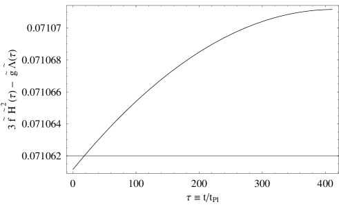
Figure 1: a) The stability criterion for the massive theory Eq.(15) assuming the MSSM particle content $N_{1,1/2,0}=(12,48,104)$, the natural value of the dimensionless $\Lambda$ at the SUSY scale (21) and a combination of extreme values of the parameters $\tilde{f}=10^{-3}$ and $\tilde{g}=-10^{2}$. b) The time dependence of $\tilde{\Lambda}(\tau)$ from the transformations Eq.(17) for the same values of the parameters as in Fig.1a.

Whether we assume the masses of the fermions and scalars to be of the same order or not, we can stipulate the parameter $\tilde{g}$ from Eq.(11) as

$$\tilde{g}\sim\pm\frac{\tilde{f}}{\Lambda_{\rm ad}}\,\sum_{s}\,\frac{\,m_{s}^{2}}{M^{2}_{\rm Pl}}\,.$$ (23)

Let us extrapolate the possible difference between the sum of the scalar masses squared and $\Lambda_{\rm ad}$, as well as the simplified approximation used in Eq.(23), in the range $(10^{-3}-10^{5})$. Thus, using Eqs.(21) and (22) we find

$$\tilde{g}\sim\pm\,(10^{-8}-10^{2})\,.$$ (24)

We begin the analysis solving the equation of motion of Eq.(9) for the dimensionless $\Lambda$ at the SUSY scale [Eq.(21)] varying $\tilde{f}$ and $\tilde{g}$ within the range of Eqs.(22) and (24), respectively. We check the stability criterion [Eq.(15)] during the inflationary period assuming the possible combinations of the range in $\tilde{f}$ and $\tilde{g}$, as well as the possibility of positive and negative signs in $\tilde{g}$ until the end of inflation which should happens at $t_{\rm end}\sim 2/H_{a}\tilde{f}$, according to the approximate parabolic solution (18). We checked that the stability criterion [Eq.(15)] is satisfied for all possible combinations of the values of the parameters. We found that $3{\tilde{f}}{\tilde{H}}^{2}(\tau)-{\tilde{g}}\,{\tilde{\Lambda}}(\tau)$ is positive until the end of inflation and the numerical solution is independent of the initial conditions. As an example, we show the stability criterion for the massive theory assuming a MSSM particle content, the natural value of the dimensionless $\Lambda$ at the SUSY scale [Eq.(21)] and a combination of extreme values of the parameters $\tilde{f}=10^{-3}$ and $\tilde{g}=-10^{2}$ in Fig.1a. The result can be understood looking at the time dependence of $\tilde{\Lambda}(\tau)$ from the transformations of Eq.(17). We notice that one can neglect the constant terms so that the function $\tilde{\Lambda}(\tau)$ has the opposite sign of $\tilde{g}$ (since $\sigma^{\prime}(\tau)=H(\tau)>0$), or ${\tilde{\Lambda}}(\tau)\propto-\tilde{g}\,\sigma(\tau)$ as shown in Fig.1b. This mean that the stability criterion is then $\sim 3{\tilde{f}}{\tilde{H}}^{2}(\tau)+{\tilde{g}}^{2}\,{\tilde{\sigma}(\tau)}$ which always has a positive sign.

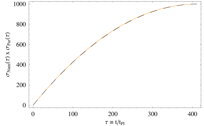
Figure 2: The numerical solution of Eq.(9) for the same values of the parameters as in Fig.1 versus the approximate parabolic solution (the dashed line).

The numerical solution of Eq.(9) can be compared to the approximate parabolic solution [Eq.(18)] for all possible combinations of the parameters values discussed above. As a result we found an accurate compatibility between the numerical and approximate solutions. We show in Fig.2 the approximate versus the numerical solution for the MSSM particle content with the same extreme values of the parameters used in Fig.1. The dashed line shows the approximate parabolic solution [Eq.(18)]. The contribution of the difference due to massive fermions and bosons, which is within the definition of $\tilde{g}$ can not be distinguished in the numerical solutions. The massive fermions are mainly responsible for slowing down $\sigma(\tau)$ and we can safely consider $\tilde{g}$ and $\Lambda$ vanishing as an approximation. The approximate solution is also robust in this stage.

5 Conclusions

We considered the inflationary solution in the modified Starobinsky (MSt) model, taking into account the cosmological constant $\Lambda$ and quantum contributions to the vacuum energy density from massive fermions and bosons. The fields with different statistics contribute with opposite signs and the overall quantum effect is due to the difference of their contributions. The natural value for $\Lambda$ corresponds to the supersymmetry breaking value at the MSSM scale. We also assumed the corresponding particle spectrum for evaluating the quantum contributions. The corresponding dimensionless parameter is called $\tilde{g}$. It turns out that the agreement between approximate analytical and numerical solutions is robust for the natural values of the above-mentioned parameters. Furthermore, the numerical solution is not sensitive to the sign of $\tilde{g}$. The latter means that the contribution of the massive fermions can be smaller or larger than the contribution of the massive boson particles without visible effect to the numerical solution of the model. The inflation remains stable until the point when the s-particles decouple and supersymmetry breaks down, for any natural choice of the parameters.

On the other hand, the renormalization of the inverse Newton constant, parametrized by the dimensionless quantity $\tilde{f}$, is very important. This parameter is always positive and its magnitude depends only on the fermion spectrum of the theory. Indeed, $\tilde{f}$ is responsible for decreasing the value of the Hubble parameter in the course of inflation.

Finally, it is very important that the value of the cosmological constant $\Lambda$ and the contributions of the massive particles do not destroy the stability which holds at the initial stage of inflation. Hence, the MSt model provides a possibility to describe all stages of inflation without fine-tuning of the parameters of the theory and/or initial data.

Acknowledgments. I am very grateful to I. L. Shapiro and R. Opher for numerous discussions and helpful comments on the manuscript and to J. Solà for useful discussions. This work has been partially supported by MEC and FEDER under project FPA2007-66665 and by DURSI Generalitat de Catalunya under project 2005SGR00564 and in part also by the Brazilian agency FAPESP (grants 2003/04516-0 and 2006/56213-9).

References

- [1] A. Friedmann, Z. Phys. 10 (1922) 377; Z. Phys. 21 (1924) 326; Gen. Rel. Grav. 31 (1999) 2001; see also, e.g., Ref. \refcitegrav.
- [2] S. Weinberg, Gravitation and Cosmology (Wiley, New York, 1972).
- [3] A. Guth, Phys. Rev. D 23 (1981) 347.
- [4] A. A. Starobinsky, Phys. Lett. B 91 (1980) 99.
- [5] N. D. Birell and P. C. W. Davies, Quantum Fields in Curved Space (Cambridge University Press, Cambridge, 1982).
- [6] I. L. Buchbinder, S. D. Odintsov and I. L. Shapiro, Effective Action in Quantum Gravity (IOP Publishing, Bristol, 1992).
- [7] M. V. Fischetti, J. B. Hartle and B. L. Hu, Phys. Rev. D 20 (1979) 1757.
- [8] A. Vilenkin, Phys. Rev. D 32 (1985) 2511.
- [9] V. F. Mukhanov and G. V. Chibisov, JETP Lett. 33 (1981) 532 [astro-ph/030307]; Sov. Phys. JETP 56 (1982) 258.
- [10] A. A. Starobinsky, JETP Lett. 30 (1979) 682; JETP Lett. 34 (1981) 438; Nonsingular Model of the Universe with the Quantum-Gravitational De Sitter Stage and its Observational Consequences Proceedings of the second seminar “Quantum Gravity”, (1982) pp. 58-72 (Moscow).
- [11] A. A. Starobinsky, Sov. Astr. Lett. 9 (1983) 302.
- [12] R. J. Riegert, Phys. Lett. B 134 (1984) 56.
- [13] E. S. Fradkin and A. A. Tseytlin, Phys. Lett. B 134 (1980) 187.
- [14] I. L. Shapiro and A. G. Jacksenaev, Phys. Lett. B 324 (1994) 284.
- [15] P. O. Mazur and E. Mottola, Phys. Rev. D 64 (2001) 104022.
- [16] I. L. Buchbinder, S. D. Odintsov and I. L. Shapiro, Phys. Lett. B 162 (1985) 92.
- [17] J. C. Fabris, A. M. Pelinson and I. L. Shapiro, Grav. Cosmol. 6 (2000) 59 (Preprint gr-qc/9810032)
- [18] J. C. Fabris, A. M. Pelinson and I. L. Shapiro, Nucl. Phys. B 597 (2001) 539.
- [19] I. L. Shapiro, Int. J. Mod. Phys. D 11 (2002) 1159.
- [20] I. L. Shapiro and J. Solà, Phys. Lett. B 530 (2002) 10.
- [21] A. M. Pelinson, I. L. Shapiro and F. I. Takakura, Nucl. Phys. B 648 (2003) 417.
- [22] R. D. Peccei, J. Solà and C. Wetterich, Phys. Lett. B 195 (1987) 183.
- [23] S. Weinberg, Rev. Mod. Phys. 61 (1989) 1.
- [24] G. E. Volovik, Int. J. Mod. Phys. D 15 (2006) 1987.
- [25] I. L. Shapiro and J. Solà, JHEP 02 (2002) 006.
- [26] S. M. Carroll, Living Rev. Rel. 4 (2001) 1 [astro-ph/0004075].
- [27] T. Padmanabhan, Phys. Rep. 380 (2003) 235.
- [28] E. J. Copeland, M. Sami and S. Tsujikawa, Int. J. Mod. Phys. D 15 (2006) 1753.
- [29] I. L. Shapiro and J. Solà, JHEP 0202 (2002) 006.
- [30] R. Opher and A. Pelinson, Int. J. Mod. Phys. D 14 (2005) 1907.
- [31] A. A. Starobinsky, Sov. Astron. Lett. 4 (1978) 82.