Dark matter and collider phenomenology of split-UED

Abstract

We explicitly show that split-universal extra dimension (split-UED), a recently suggested extension of universal extra dimension (UED) model, can nicely explain recent anomalies in cosmic-ray positrons and electrons observed by PAMELA and ATIC/PPB-BETS. Kaluza-Klein (KK) dark matters mainly annihilate into leptons because the hadronic branching fraction is highly suppressed by large KK quark masses and the antiproton flux agrees very well with the observation where no excess is found . The flux of cosmic gamma-rays from pion decay is also highly suppressed and hardly detected in low energy region ($E_{\gamma}\lesssim 20$ GeV). Collider signatures of colored KK particles at the LHC, especially $q_{1}q_{1}$ production, are studied in detail. Due to the large split in masses of KK quarks and other particles, hard $p_{T}$ jets and missing $E_{T}$ are generated, which make it possible to suppress the standard model background and discover the signals.

I Introduction

Recent observations by PAMELA PAMELA and ATIC/PPB-BETS ATIC ; PPB-BETS consistently suggest a new primary source of energetic cosmic electrons and positrons in the neighborhood of our solar system, since high energy electrons/positrons lose their energy quickly within about 1 kpc. These resutls have attracted enormous attentions and stimulated many interpretations of the primary electric source from both astrophysics and particle physics, for example, the nearby pulsars pulsar and dark matter decay decayDM or annihilation anniDM . The existing data of cosmic electrons and positrons cannot distinguish among these possibilities, and we expect that future data from cosmic-ray and accelerator experiments such as Fermi and Large Hadron Collider (LHC) will give us some clues on which interpretation is more promising and ultimately correct.

In this paper, we consider one of the most attractive models of dark matter, universal extra dimension (UED) with its minimal realization (mUED)UED ; Cheng:2002ab and a recently suggested variety split-UED split-UED . When the reflection symmetry (dubbed Kaluza-Klein parity) about the mid point of the orbifold extra dimension is exact, the lightest Kaluza-Klein particle (LKP), which is odd under the parity operation, is absolutely stable and is a good candidate of dark matter Servant:2002aq . It turns out that in most cases of universal extra dimension scenarios the LKP is the first Kaluza-Klein (KK) photon ($B_{1}$), and a pair of charged leptons is produced in the annihilation process of $B_{1}$. Interestingly enough, the mass of dark matter suggested by the ATIC/PPB-BETS data ($\sim 600-700$ GeV) exactly coincides with the one that gives the right relic density for the LKP dark matter after taking co-annihilation channels into account Kong:2005hn .

On the other hand, the measured data of the cosmic ray antiproton-to-proton flux ratio between 1 and 100 GeV by PAMELA follow the expectations from secondary production and strongly constrain contributions from dark matter particle annihilation Adriani:2008zq . Therefore it is required to naturally reduce antiproton flux in any dark matter model. Split-UED is promising in the sense that production of antiproton is quite suppressed. The cross section for dark matter annihilates into a quark pair is

$$\langle\sigma_{B_{1}B_{1}\to q\bar{q}}v\rangle\propto m_{B_{1}}^{2}/(m_{B_{1}}^{2}+m_{q_{1}}^{2})^{2}$$

where $m_{B_{1}}$ and $m_{q_{1}}$ are the masses of $B_{1}$ and the first KK quark ($q_{1}$), respectively, and it can be significantly suppressed by increasing the masses of KK quarks, i.e. splitting the KK quarks from other particles. However we should keep in mind that predictions of the observed antiprotons from dark matter annihilation can vary quite a lot for different adopted diffusion models as we will see later. As hadronic production is suppressed in split-UED, we would also expect much less production of cosmic gamma-ray whose main source is decay of pions. This prediction will be tested by forthcoming data from the Fermi experiment FGST .

The split spectrum of Kaluza-Klein particles is realized by introducing a bulk mass term for quarks in split-UED keeping the KK parity exact split-UED . One immediate consequence is that the 5D wave functions of quark fields are quasi-localized at the boundaries and induce violation of the translational symmetry along the extra dimension. Accordingly the KK number conservation is violated in the quark sector, and KK-even gauge bosons could directly couple to the zero mode quarks at the tree level, which is forbidden in mUED. KK-even bosons could be copiously produced at colliders and it is promising to discover them, for example, by the 2nd KK gluon resonance at the LHC split-UED . Another consequence is the heavy KK quark decay to the SM quark and KK boson, which will generate harder jets with large missing momentum compared to that in mUED due to a large mass splitting between KK quarks and other KK particles. Such differences may give us some handle to tell split-UED apart from mUED at the LHC.

This paper is organized as follows. In Section II we review split-UED and show how the spectrum and the interactions are modified compared with those in mUED. Note that the renormalization group (RG) running is taken into account in our spectrum calculation. We then calculate the annihilation cross section to leptons and quarks with varying “bulk mass parameter”, $\mu$, which is the only new extra parameter in split-UED. In Section III, we estimate the signals of cosmic-ray positrons, electrons, and antiprotons from LKP dark matter annihilation in both mUED Hooper:2009fj and split-UED, and compare our predictions with recent experimental data. Moreover, the diffusive gamma-ray is studied as well. In Section IV, we consider the productions of KK quarks and gluons at the LHC, and we also discuss the possibility of discovering these signals and mass reconstructions. We finally conclude our studies in Section V.

II Masses and Couplings in Split-UED

Our set-up is based on the all SM fields are “universally” propagating in one extra dimension, which is compactified on an orbifold, $S^{1}/Z_{2}$, with the boundary points $y=\pm L$ (the orbifold radius $R=2L/\pi$). The extension we have introduced is an scalar background $\Phi(y)$ that couples to each colored Dirac fermions $\Psi_{q}(x^{\mu},y)$ in the 5D bulk where the corresponding standard model quark field $q$ (=$SU(2)$ singlets $u_{R}^{c},d_{R}^{c}$ and doublet $Q_{L}$) resides on the chiral zero mode after orbifold projection. A common Yukawa coupling $\lambda(\equiv\lambda_{Q_{L}}=\lambda_{u_{R}^{c}}=\lambda_{d_{R}^{c}})$ is assumed for all quarks so that any further source of flavor violation beyond the CKM matrix is automatically avoided and the model becomes more predictive . Here we neglect the family indices but one can easily extend the model to include more generations. Finallly the 5D action is given by the form

$$S_{\rm split-UED}=\int d^{4}x\int_{-L}^{L}dy\Big{[}\mathcal{L_{\rm mUED}}-\lambda\Phi(y)\bar{\Psi}_{q}(x,y)\Psi_{q}(x,y)\Big{]}\ ,$$ (1)

where the summation runs for all quark fields $q$, and $\mathcal{L_{\rm mUED}}$ contains the usual mUED terms.

If we choose an odd background profile $\Phi(-y)=-\Phi(y)$ under the inversion symmetry about the middle point $y=0$, we can see that the KK parity, which transforms the fields as $\Phi(x,y)\rightarrow\Phi(x,-y)$, $\Psi_{q}(x,y)\rightarrow\pm\gamma_{5}\Psi_{q}(x,-y)$, is still a good symmetry of the Lagrangian. For quantitative concreteness we consider the simplest mass profile which respects the requirement: $\lambda\langle\Phi(y)\rangle=\mu\epsilon(y)$, where $\mu$ is the bulk mass parameter and $\epsilon(y)$ is a step function defined as $+1$ for $0<y<L$ and $-1$ for $-L<y<0$. As ($\lambda\to 0$) or equivalently ($\mu\to 0$), split-UED is continuously reduced to mUED thus we call this limit as “mUED limit” below. For gauge bosons, scalars, and leptons ($l$), their KK decompositions are the same as those in mUED, while for quarks, their odd masses will affect the KK decompositions. The details of the all KK decompositions in Eq. (1) are presented in Appendix A. Notice that in the case of KK decomposition, we also label the KK parity in addition to the KK number $n=\{n^{-}(\textrm{n odd}),~{}n^{+}(\textrm{n even})\}$.

The tree level mass for the $n$-th KK fermion is given by

$$m_{q_{n}}^{\textrm{tree}} = \sqrt{\mu^{2}+k_{n}^{2}},$$ (2)

$$m_{l_{n}}^{\textrm{tree}} = n/R\ ,$$ (3)

if we neglect their masses coming from electroweak symmetry breaking. Here $k_{n}$ is determined by the boundary conditions which are given by:

$$k_{n^{-}} = -|\mu|\tan{k_{n}L},$$ (4)

$$k_{n^{+}} = n/R\ .$$ (5)

We choose the minimal universal boundary conditions at the energy cutoff scale $\Lambda$ that all boundary kinetic terms vanish , and the general expression for the one-loop correction to the $n$-th KK fermion masse is given by Cheng:2002iz

$$m_{f_{n}}=m_{f_{n}}^{\textrm{tree}}\left[1+\frac{9}{8\pi}\left(\sum_{G}C_{2}^{G}(N)\alpha_{G}\right)\log\Lambda R\right]\ ,$$ (6)

where $\alpha_{G}=g_{G}^{2}/4\pi$ and we neglect the Yukawa corrections in this formula. The sum is over all SM gauge groups under which the fermion $f$ is charged, and $C_{2}^{G}(N)$ is the quadratic Casimir operator of the fundamental representation $N$ in gauge group $G$, e.g., $C_{2}^{SU(N)}(N)=(N^{2}-1)/2N$ and we take $C_{2}^{U(1)_{Y}}(N)=Y_{f}^{2}$ with $Y_{f}$ being the hypercharge of $f$. If we choose $(\alpha_{1},\alpha_{2},\alpha_{3})\simeq(0.010,0.033,0.094)$ at $Q^{2}=(620{\rm GeV})^{2}$, colored particles will get bigger corrections ($\sim 14\%$ for $u_{R}^{1},d_{R}^{1}$ and $16\%$ for $Q_{L}^{1}$) than leptons ($\sim 1.9\%$ for $l_{R}^{1}$ and $3.1\%$ for $l_{L}^{1}$).

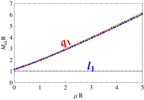
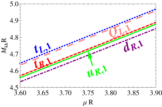
Figure 1: (upper plot) The spectra of 1st KK quarks and leptons in the unit $1/R$ with the given bulk mass parameter $\mu$. The lepton masses are independent of $\mu$ in our scenario. Here we included 1-loop correction for all the masses. The most important correction is QCD correction and it is roughly $14\sim 16\%$ for quarks. For leptons the correction is small ($\sim 2\%$). (lower plot) The magnified figure of the upper one in $\mu R=(3.60,3.90)$. $SU(2)$ doublets ($t_{L},Q_{L}$) get the larger 1-loop correction than singlet quarks ($u_{R},d_{R}$) get.

In Fig. 1 we plot the spectra of 1st KK quarks and leptons including 1-loop corrections. When $\mu=0$, i.e. the mUED limit, quarks are quite degenerate with leptons even we take the QCD corrections to the masses into account. However when we increase the bulk mass parameter $\mu$, the KK quark masses become larger and larger so that we get the split spectra as we request. Note that small deviations in quark spectra come from different $SU(2)$ and $U(1)$ charge of $u_{R},d_{R}$ and $Q_{L}$. In our study, these differences can be neglected.

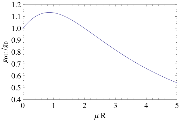
Figure 2: The coupling constant ratio $g_{A_{1}-q_{1}-q_{0}}/g_{0}={\cal G}_{110}$ vesus $\mu R$. The dependence comes from the change of the 5D profiles. Notice that the coupling ratio first increases to its maximal value around 1.14 for $\mu R\sim 1$ and then decreases monotonically.

The couplings between KK gauge bosons and fermions determine the most interesting phenomenological features of the model. All 4D effective couplings could be calculated by integrating out the 5D profiles of the relevant fields along the extra dimension. Since 5D profiles are the same for different KK gauge bosons (quarks) with the same KK number, the ratio between a general gauge boson-quark-quark coupling $g_{A_{m}-q_{n}-q^{\prime}_{l}}$ over the SM one is the same for fixed KK numbers, where $m$, $n$ and $l$ are KK number of $A$, $q$ and $q^{\prime}$, respectively. We introduce a function $\mathcal{G}_{mnl}(\mu R)$ to parameterize how such a ratio depends on the bulk mass parameter $\mu$ times the radius $R$:

$$g_{A_{m}-q_{n}-q_{l}}/g_{0}\equiv{\cal G}_{mnl}(\mu R)\ ,$$ (7)

where $g_{0}$ is the SM gauge interaction between $A_{0}$, $q_{0}$ and $q^{\prime}_{0}$. Among those couplings, the most interesting one in phenomenology is the coupling between the 1st KK gauge boson $A_{1}$, the 1st KK quark $q_{1}$, and SM quark $q_{0}$, which is crucial on LKP pair annihilation and productions of $q_{1}$ and the 1st KK gluon $g_{1}$ at the LHC. The dimensionless function ${\cal G}_{110}(\mu R)$ is calculated from the 5D profiles of $A_{1}$, $q_{1}$ and $q_{0}$ given by Eq. (37), (38), (Appendix A: KK decomposition in split-UED), and (41) in Appendix A, and is plotted in Fig. 2 as a function of $\mu R$. At $\mu=0$ limit we get the mUED result, which is the same as the SM coupling. As $\mu$ gets larger, the 5D profiles are localized so that the resultant overlap among the fields get smaller.

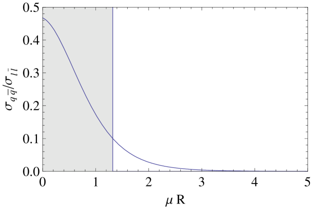
Figure 3: The ratio of LKP pair annihilation into quarks and charged leptons vesus $\mu R$. The mUED limit corresponds to $\mu=0$ and the ratio of cross section to quarks to leptons is about $47\%$ but it quickly goes down below $10\%$ as $\mu\mathrel{\hbox to0.0pt{\lower 4.0pt\hbox{\hskip 1.0pt$\sim$}\hss}\raise 1.0pt\hbox{$>$}}1.3/R$. The shaded region ($\sigma_{q\bar{q}}/\sigma{l\bar{l}}>10\%$) is not preferred by PAMELA antiproton data.

Table 1: The branching fraction of the LKP pair annihilates into various final states, for different $q_{1}$ mass, and different bulk mass parameter $\mu$. The numbers shown are summed over generations. We neglect the $W$-boson final state because the SU(2) component of LKP is too small. Here we fix the LKP mass to be 620 GeV and include the radiative corrections to all the masses according to Ref. Cheng:2002iz .

$\mu$ (GeV)	0	200	400	600	800	1000
$M_{q_{1}}$ (GeV)	713	863	1026	1198	1378	1566
BR($B_{1}B_{1}\rightarrow q\bar{q}$)	29.4%	26.4%	20.6%	14.3%	8.9%	5.2%
BR($B_{1}B_{1}\rightarrow l\bar{l}$)	64.3%	67.1%	72.3%	78.2%	83.0%	86.5%
BR($B_{1}B_{1}\rightarrow\nu\bar{\nu}$)	3.8%	3.9%	4.3%	4.6 %	4.9%	5.1%
BR($B_{1}B_{1}\rightarrow\phi\phi^{*}$)	2.3%	2.4%	2.6%	2.8%	3.0%	3.1%

Taking care of all the corrections and effects of $\mu$ we can now calculate the branching fractions that LKP pair annihilates into quarks and leptons. At the non-relativistic limit ($\beta=\sqrt{1-4m_{B_{1}}^{2}/s}\rightarrow 0$), the cross section for LKP pair annihilates into fermions can be well approximated as:

$$\langle\sigma v\rangle_{B_{1}B_{1}\rightarrow f\bar{f}}=\frac{2g_{1}^{4}C_{f}}{9\pi m_{B_{1}}^{2}}\left[\frac{\mathcal{G}_{110}(\mu R)}{(1+r_{f}^{2})}\right]^{2}+{\cal O}(v),$$ (8)

where a useful numerical term $C_{f}=N_{c}(Y_{f_{L}}^{4}+Y_{f_{R}}^{4})$ is introduced with the color factor $N_{c}=3(1)$ for quarks(leptons). The mass ratio between the LKP and KK fermion is parameterized by a parameter $r_{f}$ defined as $r_{f}\equiv m_{f_{1}}/m_{B_{1}}$ and we ignore the small mass corrections coming from $SU(2)_{L}$, $U(1)_{Y}$ gauge group so that $m_{f_{1}}=m_{f_{L1}}\simeq m_{f_{R1}}$. In mUED limit, the ratio between productions of the lepton and the quark is mainly controlled by the ratio of $C_{f}$ from the hypercharges and color factor of fermions. For leptons and quarks the corresponding terms are $\sum_{l}C_{l}\simeq 3.18$ and $\sum_{q}C_{q}\simeq 1.90$, respectively. Obviously the mUED does have a sizable hadronic annihilation channel and a carefully study of antiproton flux is important. In the case of split-UED, one can easily adjust $r_{q}$ to suppress the hadronic annihilation cross section. In Fig. 3 we plot the ratio of annihilation cross section into quarks and charged leptons $\sigma_{q\bar{q}}/\sigma_{l\bar{l}}$ with $\mu R$ in the range of $(0,5)$. We find the ratio goes down very quickly as the bulk mass parameter goes larger since $\sigma\sim 1/(1+r_{f}^{2})^{2}$. By turning on the bulk mass parameter we can easily avoid the antiproton excess in the cosmic ray detection experiments. We also note that the soft gamma-ray from decay of hadrons, especially from pions, is under control in this set-up.

III Cosmic Positron, Antiproton and Photon

LKP dark matter $B_{1}$ will mainly annihilate into a fermion pair while the W-boson and Higgs boson modes are suppressed, as shown in Table 1. For the quark-pair final state, due to the QCD hadronization process, a bunch of hadrons will be produced and sequentially decay into positrons/electrons, protons/antiprotons, photons and neutrinos. Moreover, positrons and electrons also originate in the leptonic channels: muon and tau (also generate photons) decay and direct production in $B_{1}B_{1}\to e^{+}e^{-}$ process. In our calculation, we use PYTHIA Sjostrand:2006za for the simulation of the QCD hadronization and the decays of particles. Since these stable particles from the dark matter annihilation in our Galaxy will propagate to our solar system and be observed as cosmic-ray signals, we estimate the predictions from our model, the split-UED, and compared with experimental data in this section. Due to the fact that excesses were observed in the positron fraction in PAMELA PAMELA and the flux of electron plus positron in ATIC/PPB-BETS ATIC ; PPB-BETS while the ratio of antiproton to proton, $\bar{p}/p$, is consistent with the astrophysical background, we first explain positron and electron data from the dark matter annihilation. Then base on the parameters set by fitting the ATIC/PPB-BETS and PAMELA data, we calculate the $\bar{p}/p$ and photon flux. Since the W-boson and the Higgs boson productions are highly suppressed in UED models we are considering, we will not take into account their contributions in the following calculations.

III.1 Positron and Electron

Model	$\delta$	$K_{0}(\rm{kpc^{2}/Myr})$	$L(\rm{kpc})$
M2	$0.55$	$0.00595$	$1$
MED	$0.70$	$0.0112$	$4$
M1	$0.46$	$0.0765$	$15$

Table 2: The parameters in the diffusion models which are comparible with B/C and generate minimum (M2), median (MED) and maximal (M1) positron flux.

In this section, we calculate the cosmic-ray positrons and electrons from the $B_{1}B_{1}$ annihilation which account for the PAMELA and ATIC/PPB-BETS data. Since the dark matter annihilation generates the same amount of electrons and positrons, we only show the formula for positron flux below. After being produced from the dark matter annihilation process, the positrons will propagate in the magnetic field of the Milky Way. Because the magnetic fields are tangled, the motion of the positron can be described by a diffusion equation. Neglecting the convection and annihilation in the disk, the steady state solution must satisfy

$$K(E)\bigtriangledown^{2}f_{e^{+}}(E,\vec{r})+\frac{\partial}{\partial E}\left[b(E)f_{e^{+}}(E,\vec{r})\right]+Q(E,\vec{r})=0,\,$$ (9)

where $f_{e^{+}}$ is the number density of $e^{+}$ per unit kinetic energy, $K(E)=K_{0}(E/\rm{GeV})^{\delta}$ is the diffusion coefficient, $b(E)=10^{-16}(E/\rm{GeV})^{2}$ is the rate of energy loss and $Q(E,\vec{r})$ is the source of producing $e^{+}$. In the $B_{1}$ dark matter annihilation case,

$$Q(E,\vec{r})=\frac{1}{2}\left(\frac{\rho(\vec{r})}{m_{B_{1}}}\right)^{2}\sum_{i}\langle\sigma v\rangle_{i}\left(\frac{dN(E)_{e^{+}}}{dE}\right)_{i},$$ (10)

where $dN_{e^{+}}/dE$ is the energy spectrum of $e^{+}$ obtained by using PYTHIA, the index $i$ runs over all quark and charged lepton pairs and $\rho(\vec{r})$ is the dark matter profile. In our numerical calculations, we adopt an overall boost factor $B_{F}$ and the isothermal halo model Bergstrom:1997fj which is given as

$$\rho_{\textrm{halo}}(\vec{r})=\frac{\rho_{0}}{1+(r/r_{c})^{2}},$$ (11)

where $r=|\vec{r}|$ is the distance from our Galactic center, $r_{c}=3.5$ kpc and $\rho_{0}$ is the parameter that is adjusted to yield a dark matter local halo density of $0.3\,\rm{GeV}/cm^{3}$ Bergstrom:1997fj in our solar system. Considering the diffusion zone of a cylinder with radius R and half-height L, the solution for the positron flux at the Earth can be written in a useful form Hisano:2005ec

$$\Phi^{DM}_{e^{+}}(E)=\frac{c}{4\pi}f_{e^{+}}(E,r_{\odot}),\,$$ (12)

where $c$ is the speed of light,

$$f_{e^{+}}(E,r_{\odot})=\int_{E}^{m_{B_{1}}}\frac{10^{16}}{E^{2}}dE^{\prime}\sum_{n,m=1}^{\infty}Q_{n,m}(E^{\prime})J_{0}\left(\frac{\zeta_{n}r_{\odot}}{R}\right)\sin\left(\frac{m\pi}{2}\right)\exp\left[\left((\frac{m\pi}{2L})^{2}+(\frac{\zeta_{n}}{R})^{2}\right)X\right]$$ (13)

where $E^{(^{\prime})}$ is the energy in a unit of GeV, $J_{0}$ is the zeroth-order of the first kind Bessel function, $r_{\odot}\sim 8.5$ kpc is the distance from Milky Way center to the Sun, $\zeta_{n}$ is the n-th zero of the function $J_{0}$,

$$X=\frac{K_{0}\times 10^{16}}{\delta-1}\left[E^{\delta-1}-E^{\prime\delta-1}\right]$$ (14)

and

$$Q_{n,m}(E)=\frac{2}{J_{1}(\zeta_{n})^{2}R^{2}L}\int_{0}^{R}drrJ_{0}(\frac{\zeta_{n}r}{R})\int_{-L}^{L}dz\sin\left(\frac{m\pi z}{2L}(L-z)\right)Q(E,\vec{r}).$$ (15)

The $J_{1}$ in the Eq.(15) is the first-order of the Bessel function and the parameters $\delta,K_{0}$ are set in the simulations of diffusion models to coincide with the observed cosmic-ray data, especially the Boron to Carbon ratio (B/C) Maurin:2001sj . The values for different diffusion models we adopted are listed in table 2 Delahaye:2007fr .

In addition to $e^{\pm}$ fluxes from dark matter annihilation, there exist secondary $e^{\pm}$ fluxes from interactions between cosmic-rays and nuclei in the interstellar medium. We use the approximations of the $e^{-}$ and $e^{+}$ background fluxes  Moskalenko:1997gh ; Baltz:1998xv

$$\Phi_{e^{-}}^{prim}(E) =\frac{0.16E^{-1.1}}{1+11E^{0.9}+3.2E^{2.15}}\quad{\rm GeV}^{-1}{\rm cm}^{-2}{\rm sec}^{-1}{\rm sr}^{-1},$$

$$\Phi_{e^{-}}^{sec}(E) =\frac{0.7E^{0.7}}{1+110E^{1.5}+600E^{2.9}+580E^{4.2}}\quad{\rm GeV}^{-1}{\rm cm}^{-2}{\rm sec}^{-1}{\rm sr}^{-1},$$

$$\Phi_{e^{+}}^{sec} (E)=\frac{4.5E^{0.7}}{1+650E^{2.3}+1500E^{4.2}}\quad{\rm GeV}^{-1}{\rm cm}^{-2}{\rm sec}^{-1}{\rm sr}^{-1},\,$$ (16)

where $E$ is in units of GeV. Therefore, the fraction of positron flux and total flux of positron plus electron are

$$\frac{\Phi_{e+}^{DM}+\Phi_{e+}^{sec}}{\Phi_{e+}^{DM}+\Phi_{e-}^{DM}+\Phi_{e+}^{sec}+k\Phi_{e^{-}}^{prim}+\Phi_{e^{-}}^{sec}},\,$$ (17)

and

$$\Phi_{e+}^{DM}+\Phi_{e-}^{DM}+\Phi_{e+}^{sec}+k\Phi_{e^{-}}^{prim}+\Phi_{e^{-}}^{sec},\,$$ (18)

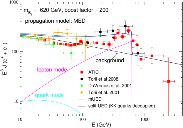
Figure 4: The flux of electron plus positron from LKP dark matter annihilation using MED diffusion model, compared with experimental data DuVernois:2001bb ; Torii:2001aw ; PPB-BETS ; ATIC . Note that only lepton mode is inclulded in the split-UED, since all the KK quarks are decoupled.

respectively, where $k$ is a free parameter which is used to fit the data when no primary source of $e^{+}$ flux exists Baltz:1998xv ; Baltz:2001ir . For our numerical simulation, we take the mass of dark matter, $m_{B_{1}}$ to be $620$ GeV. In Fig.4, we show the total flux of electron and positron with the background from Eq.(16) and recent experimental data DuVernois:2001bb ; Torii:2001aw ; PPB-BETS ; ATIC . In order to have a better fit for the data, a boost factor of 200 is needed, which is consistent with the value (200) chosen in Ref.ATIC . Boost factor is known to have origins such as local clumps in dark matter profile clump1 (see also clump2 ), Sommerfeld enhancement effect by a long range attractive force Sommerfeld1 ; Sommerfeld2 ; Sommerfeld3 ; Sommerfeld4 ; Sommerfeld5 , the Breit-Wigner type resonance effect Breit-Wigner and possibly many more origins. In our case, without assuming a new attractive force or further tuning of mass spectra to get the large resonance, we tend to assume that boost factor mainly comes from clumps. We also show in Fig.4 the contributions of quark mode and leptonic mode from the dark matter annihilation. The $e^{\pm}$ from quark mode are much softer than that in the leptonic mode. This is because that the main source of $e^{\pm}$ in quark mode is the hadron cascade decay while in leptonic mode there exists a direct production of $B_{1}B_{1}\to e^{+}e^{-}$, and $e^{\pm}$ from $\mu^{\pm}$ and $\tau^{\pm}$ decay are harder. We can easily see that the peak is mainly contributed by the leptonic mode and sharp drop-off is due to the direct production of $e^{\pm}$, therefore, the predictions of mUED and split-UED are quite similar to each other in the peak region since the difference between these two models is just in quark sector. We also compare different diffusion models in Fig.5 for split-UED case. MED and M1 models produce more soft electrons and positrons than the M2 model does, thus the distributions of the former two models are flater. For energetic positrons and electrons, all of three models are quite the same with each other.

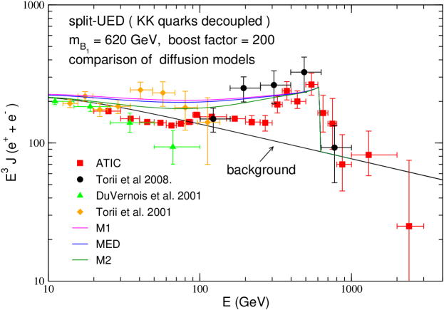
Figure 5: The same as Fig.4 but only for split-UED, and different diffusion models, M1, MED and M2, are shown together.

For positron fraction, we show in Fig.6 the predictions of mUED and split-UED, using MED diffusion model, with PAMELA data PAMELA . Since there are more soft $e^{+}$ in mUED from the quark modes, the distribution is falter compared to that of split-UED. If we adopt M2 and M1 models, as shown in Fig.7, the fittings seem worse compared the MED case for split-UED especially in the energy region around $10$ GeV. However, we have decoupled all of the higher KK quarks in this plot, i.e. hadronic final states are turned off in the dark matter annihilation. With finite mass of a first KK quark, more soft positrons will be produced, therefore, the M2 model can also be consistent with the data. For M1 model, we expect that by tuning the parameters, e.g. boost factor or the normalization of the background, it would be possible to explain the PAMELA data as well. So, we conclude here that the dark matter in both mUED and spilt-UED can be the equivalently good source of the excesses in PAMELA and ATIC/PPB-BETS data.

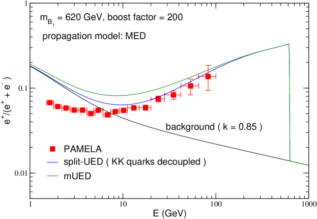
Figure 6: The positron flux fraction predicted from the LKP dark matter annihilation using MED diffusion model, compared with PAMELA data PAMELA .

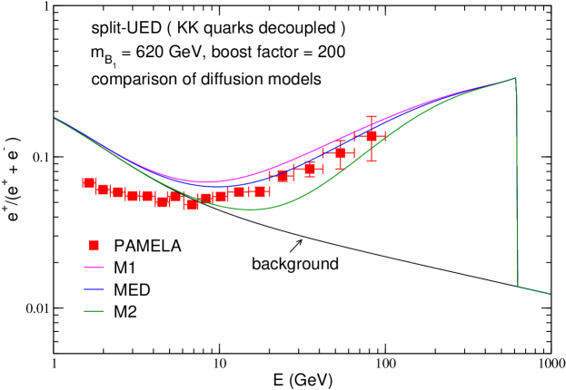
Figure 7: Same as Fig.6 but only for split-UED, and different diffusion models, M1, MED and M2, are shown together.

III.2 Antiproton

The propagation of antiprotons through the Galaxy is similar to that of positrons. The diffusion equation of antiprotons can be described as

$$K_{p}\bigtriangledown^{2}f_{\bar{p}}(T,\vec{r})-\frac{\partial}{\partial z}\left[(sign\,of\,z)V_{c}(z)f_{\bar{p}}(T,\vec{r})\right]-2h\delta(z)\Gamma_{ann}f_{\bar{p}}(T,\vec{r})+Q(T,\vec{r})=0,\,$$ (19)

where $f_{\bar{p}}(T,\vec{r})$ is the number density of antiproton per unit energy, $T$ is the kinetic energy of antiproton and $K_{p}=K_{0p}\beta(p/\rm{GeV})^{\delta}$ is the diffusion parameter. $V_{c}(z)$ in the second term of Eq.(19) is related to the convective wind that tends to push antiprotons away from the Galactic plane, and is assumed to be a constant . Again, like the case in positron, the values of $K_{0p}$, $\delta$ and $V_{c}$ for different diffusion models are set to agree with the observed cosmic-ray data, especailly the B/C, and their values are listed in table 3 Delahaye:2007fr . The third term of Eq.(19) represents the annihilation of $\bar{p}$ with the interstellar proton in the Galactic plane, $h$ is the half-height of plane which is set to be $0.1$ kpc in our calculations. The antiproton annihilation rate $\Gamma_{ann}$ is given as Donato:2001ms

$$\Gamma_{ann}=(n_{H}+4^{2/3}n_{He})\sigma^{ann}_{\bar{p}p}(T)v_{\bar{p}},$$ (20)

where $n_{H}\sim 1/\rm{cm}^{3}$ and $n_{He}\sim 0.07n_{H}$ are the number densities of hydrogen and helium, respectively; $\sigma^{ann}_{\bar{p}p}(T)$ is the annihilation cross section and $v_{\bar{p}}$ is the velocity of antiproton. The form of $\sigma^{ann}_{\bar{p}p}(T)$ is given by Tan:1983de

$$\sigma^{ann}_{\bar{p}p}(T)=\left\{\begin{array}[]{cc}661(1+0.0115T^{-0.774}-0.948T^{0.0151})\,\rm{mbarn}&,\rm{for}\,T<15.5\,{\rm{GeV}};\\ 36T^{-0.5}\,\rm{mbarn}&,\rm{for}\,T\geq 15.5\,{\rm{GeV}}.\end{array}\right.$$ (21)

The solution of the interstellar flux of antiproton in the vicinity of solar system is Cirelli:2008id

$$\Phi^{\rm{IS}}(T) = \frac{v_{\bar{p}}}{4\pi}f_{\bar{p}}(T,\vec{r_{\odot}})$$

$$= \frac{v_{\bar{p}}}{4\pi}\frac{1}{2m_{B_{1}}^{2}}\sum_{i}<\sigma v>_{i}G(T)\left(\frac{dN_{\bar{p}}}{dT}\right)_{i},$$

where the $dN_{\bar{p}}/dT$ is the spectrum of antiproton which we simulate with PYTHIA, and the index $i$ runs over all quark final states in the $B_{1}$ dark matter annihilation processes, and

$$G(T)=\sum_{n,m=1}^{\infty}J_{0}\left(\zeta_{n}\frac{r_{\odot}}{R}\right)\exp\left[-\frac{V_{c}L}{2K_{p}(T)}\right]\frac{y_{n}(L)}{A_{n}\sinh(S_{n}L/2)},$$ (23)

with

$$y_{n}(L)=\frac{4}{J_{1}^{2}(\zeta_{n})R^{2}}\int_{0}^{R}drrJ_{0}(\zeta_{n}r/R)\int_{0}^{L}dz\exp\left[\frac{V_{c}(L-z)}{2K_{p}(T)}\right]\sinh(S_{n}(L-z)/2)\rho(\vec{r})^{2},$$ (24)

and

$$A_{n} = 2h\Gamma_{ann}+V_{c}+K_{p}(T)S_{n}\coth(S_{n}L/2),$$ (25)

$$S_{n} = \sqrt{\frac{V_{c}^{2}}{K^{2}_{p}(T)}+\frac{4\zeta_{n}^{2}}{R^{2}}}.$$ (26)

However, we have to take solar modulation into account to estimate the flux of antiproton obtained at the the Earth, which is important for the low energy antiproton. The flux of the antiprotons at the top of Earth’s atmosphere can, therefore, be written as ap:solar1 ; ap:solar2

$$\Phi_{\bar{p}}^{\rm{TOA}}(T_{\rm{TOA}})=\frac{2m_{p}T_{\rm{TOA}}+T_{\rm{TOA}}^{2}}{2m_{p}T_{\rm{IS}}+T_{\rm{IS}}^{2}}\Phi_{\bar{p}}^{\rm{IS}}(T_{\rm{IS}}),$$ (27)

where $T_{\rm{TOA}}=T_{\rm{IS}}-\phi_{F}$ with $\phi_{F}$ being the solar modular parameter which we take to be $500$ MV in our calculation.

Model	$\delta$	$K_{0p}(\rm{kpc^{2}/Myr})$	$L(\rm{kpc})$	$V_{c}(\rm{km/s})$
MIN	$0.85$	$0.0016$	$1$	$13.5$
MED	$0.70$	$0.0112$	$4$	$12$
MAX	$0.46$	$0.0765$	$15$	$5$

Table 3: The parameters in the diffusion models which are comparible with B/C and generate minimum (MIN), median (MED) and maximal (MAX) antiproton flux.

In order to compare with the observed data of antiproton to proton ratio, we need to include the astrophysical background. Here we adopt simple fittings for background antiprotons $\Phi_{\bar{p}}^{bg}$ and protons $\Phi_{p}^{bg}$ provided in Ref.Nezri:2009jd ,

$$\Phi_{\bar{p}}^{bg} = \frac{0.9t^{-0.9}}{14+30t^{-1.85}+0.08t^{2.3}}\,[\rm{GeV}^{-1}\rm{m}^{-2}\rm{s}^{-1}\rm{sr}^{-1}],$$ (28)

$$\Phi_{p}^{bg} = 10^{4}\frac{0.9t^{-1}}{8+1.1t^{-1.85}+0.8t^{1.68}}\,[\rm{GeV}^{-1}\rm{m}^{-2}\rm{s}^{-1}\rm{sr}^{-1}].$$ (29)

The predicted ratios of antiproton to proton, $\bar{p}/p$, for mUED and split-UED are shown in Fig. 8 with experimental data Adriani:2008zq ; Orito:1999re ; Boezio:2001ac ; Asaoka:2001fv ; Abe:2008sh . Here we take a common boost factor ($B_{F}=200$) which we have obtained from ATIC/PPB-BETS fit. Since the hard electronic signals are mainly from local sources within a few kpcs but antiprotons can come from distant sources, one may take different values of boost factor for positron and antiproton in one’s calculation. Here, partly for predictability and simplicity and partly in order to follow common assumption that we live at a typical place in our galaxy, we take a common boost factor for all particles in our calculations. The mUED agrees well in the low energy region $E\lesssim 10$ GeV, but starts deviating significantly from the recent PAMELA data when energy of antiproton becomes higher, if MED diffusion model is adopted. Therefore, mUED seems to be disfavored by PAMELA data in the high energy region, and it agrees with PAMELA observations only when MIN diffusion model is chosen. However, one can easily see that how the situation can be improved in the split-UED case. By enhancing the mass of $q_{1}$ to be twice of the $l_{1}$, the prediction of $\bar{p}/p$ is reduced by more than a factor of two, and will be much suppressed if $q_{1}$ becomes heavier, as shown by the blue and magenta lines in Fig.8. We also note that if we adopt MIN model, the split-UED case agrees with PAMELA very well even for $m_{q_{1}}=2m_{l_{1}}$. The lower bound of the mass of $q_{1}$ in split-UED can be estimated by the upcoming data of PAMELA in the higher energy region, since a small bump is predicted at $E\approx 200$ GeV, and the height of deviation from background is controlled by the mass of $q_{1}$.

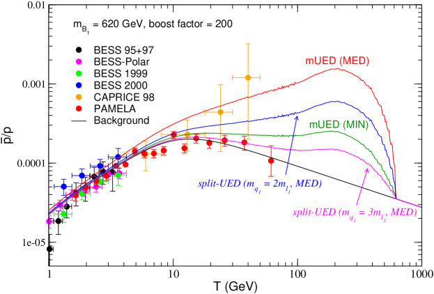
Figure 8: Antiproton to proton ratio predicted in mUED and split-UED models, together with experimental data. In mUED, both MED (red line) and MIN (green line) diffusion models are shown. For split-UED, the cases of $m_{q_{1}}=2m_{l_{1}}$ (blue line) and $m_{q_{1}}=3m_{l_{1}}$ (magenta line) are presented, using MED diffusion model.

III.3 Gamma-ray

For diffusive gamma-ray, there are galactic and extragalactic contributions from the annihilation of LKP dark matter $B_{1}$. The flux of the gamma-ray from the extragalactic origin is estimated as Bergstrom:2001jj

$$\left[E^{2}\frac{dJ_{\gamma}}{dE}\right]_{eg}=\frac{B_{F}E^{2}c\Omega_{B_{1}}^{2}\rho_{c}^{2}}{4\pi m_{B_{1}}^{2}H_{0}\Omega_{M}^{1/2}}\sum_{i}<\sigma v>_{i}\int_{0}^{z_{{\rm up}}}dy\left(\frac{dN_{\gamma}}{d((1+z)E)}\right)_{i}\frac{(1+z)^{-3/2}e^{-z/z_{\rm{max}}}}{\sqrt{1+\frac{\Omega_{\Lambda}}{\Omega_{M}}(1+z)^{-3}}},$$ (30)

where $\Omega_{B_{1}}$, $\Omega_{M}$ and $\Omega_{\Lambda}$ are the density parameters of $B_{1}$, matter (including both baryons and dark matter) and the cosmological constant, respectively; $\rho_{c}$ is the critical density; $H_{0}$ is the Hubble parameter at the present time; $z$ is the redshift, and $z_{up}=m_{B_{1}}/E-1$ since the maximum energy of photon in the rest frame of annihilation is $E=m_{B_{1}}$; the term $e^{-z/z_{\rm{max}}}$ with $z_{\rm{max}}(E)\sim 3.3(E/10\rm{GeV})^{-0.8}$ takes the optical depth into account Bergstrom:2001jj . For the numerical results, we use Komatsu:2008hk

$$\Omega_{B_{1}}h^{2}=0.1099,\quad\Omega_{M}h^{2}=0.1326,\quad\Omega_{\Lambda}=0.742,\quad\rho_{c}=1.0537\times 10^{-5}{\rm GeV/cm}^{3}.\,$$ (31)

On the other hand, the gamma-ray flux from the annihilation of $B_{1}$ in the Milky Way halo is

$$\left[E^{2}\frac{dJ_{\gamma}}{dE}\right]_{halo}=\frac{E^{2}}{4\pi}\frac{1}{2m_{B_{1}}^{2}}\frac{dN_{\gamma}}{dE}\left\langle\int_{los}\rho^{2}(\vec{\ell})d\vec{\ell}\right\rangle,$$ (32)

where $\rho_{halo}$ is the density profile of dark matter in the Milky Way, $\left\langle\int_{los}\rho^{2}(\vec{\ell})d\vec{\ell}\right\rangle$ is the average of the integration along the line of sight (los).

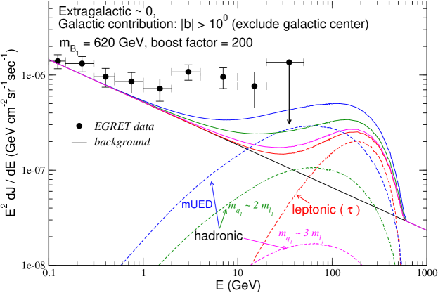
Figure 9: The diffusive gamma-ray predicted in mUED and split-UED models, together with EGRET data. The solid lines are for signals with background, blue line is for mUED; green, magenta and red lines are for $m_{q_{1}}=2m_{l_{1}}$, $m_{q_{1}}=3m_{l_{1}}$ and $m_{q_{1}}\to\infty$, respectively. Signals of dark matter annihilation are shown separately in dashed lies for leptonic final state (red), hadronic final states in mUED (blue) and in split-UED with $m_{q_{1}}=2m_{l_{1}}$ (green) and $m_{q_{1}}=3m_{l_{1}}$ (magenta).

Since there are still big uncertainties and ambiguities for modeling the Galaxy center, we integrate over the whole sky except for the zone of the Galactic plane (i.e. exclude the region with the galactic latitudes $|b|<10^{\circ}$). For the background, we use a power-law form adopted in Ref. Ishiwata:2008cu

$$\left[E^{2}\frac{dJ_{\gamma}}{dE}\right]_{bg}\simeq 5.18\times 10^{-7}E^{-0.499}\quad{\rm GeVcm}^{-2}{\rm sr}^{-1}{\rm sec}^{-1},$$ (33)

where $E$ is in units of GeV.

The total flux of diffusive gamma-ray is shown in Fig.9, and the signals from the hadronic and leptonic final states in $B_{1}B_{1}$ annihilation are presented as well. We should emphasize that we do not try to fit EGRET data  Sreekumar:1997un ; Strong:2004ry in the plot, since Fermi  FGST is expected to have more precise results soon, however, we still show EGRET data for reference. We notice that the extragalactic contribution from cosmological distance is very small even we enhance it by a factor of $10^{6}$ to estimate the effect of subhalo Bergstrom:2001jj . The gamma-ray in the decay of $\pi^{0}$ from hadron cascade decay is softer than that from the decay of $\tau$, therefore the distribution become flater when more quarks are produced in $B_{1}$ annihilation. By suppressing the fraction of the quark mode in the final state, i.e. comparing mUED (blue lines) and split-UED (green, magenta and red lines), the starting point of deviation from the background will shift to high energy and the predicted peak at energy about 200 GeV will become smaller. The bump at the high energy is a generic prediction for split-UED even all of the higher order KK quarks are decoupled, because gamma-rays still come from the $\tau$ decay, and it can be further examined by the Fermi experiment in the near future.

IV Collider signature of split-UED

Having light colored particles below a few TeV in split-UED, the LHC can produce lots of KK quarks and gluons via QCD interactions. As it is already shown in Sec. II, one of the features of our model is that KK quarks are split from the other particles, therefore, will lead to collider phenomenology quite different from the mUED models. For example, the 1st KK quark, where we take $m_{q_{1}}\approx 2m_{B_{1}}$ through calculations, mainly decays to the 1st KK gluon $g_{1}$ and a SM quark, generating at least one high $p_{T}$ jet due to the big mass gap between $q_{1}$ and $g_{1}$. Another one is the existance of tree-level KK number non-conserved interactions between KK-even gauge bosons and the SM fermions, as a result, the production cross sections of 2nd KK gauge bosons can be substantial. It has been shown that the signals of a 2nd KK gluon production can be dominant over the SM background in dijet events after imposing a certain set of cuts at the LHC split-UED . In this section, we will focus on the scenarios of 1st KK quarks and gluon, which can only be produced in pairs.

Figure 10: The cross sections and the mass of $u_{L1}$ as functions of the bulk mass $\mu$ with fixing $1/R=620$ GeV. Here, $u_{1}$($d_{1}$) includes both $u_{L1}$ and $u_{R1}$ ($d_{L1}$ and $d_{R1}$) contributions.

The production cross sections involving $q_{1}$ at the LHC depend on the bulk mass parameter $\mu$. Among the production cross sections of $q_{1}q_{1}^{(\prime)}$, $q_{1}\bar{q}_{1}^{(\prime)}$ and $\bar{q}_{1}\bar{q}_{1}^{(\prime)}$, the $\sigma(q_{1}q_{1})$ is dominant one as the valence $u$ and $d$ partons can contribute to the initial states. These productions proceed mainly through the $t$-channel diagrams with the 1st KK gauge bosons exchanged. The most relevant couplings for these productions are $q_{1}$-$q$-$V_{1}$, where $V_{1}=g_{1}$, $B_{1}$, the 1st KK $W-$boson $W_{1}$ and the 1st KK $Z-$boson $Z_{1}$. The cross section $\sigma(u_{1}u_{1})$, $\sigma(u_{1}d_{1})$ and $\sigma(d_{1}d_{1})$ are plotted in Fig. 10 with varying $\mu$, and we neglect the $q_{1}\bar{q}_{1}^{(\prime)}$ productions, since they are insignificant. For small $\mu$, the production cross sections increase with increasing $\mu$ due to the enhancement from the couplings, as shown in Fig.3, since the cross section is proportional to $({\cal G}_{110})^{4}$. For large $\mu$, on the other hand, those cross sections decrease very quickly with increasing $\mu$ (increasing $m_{q_{1}}$) as expected. For the $g_{1}q_{1}$ and $g_{1}g_{1}$ productions, the cross sections, which are not shown, are at the same order as that of $q_{1}q_{1}$. Here all cross sections are calculated using CalcHEP Pukhov:2004ca by modifying the mUED model file in Ref. mUEDcalc .

The signature of split-UED $q_{1}q_{1}$ productions followed by $q_{1}\rightarrow g_{1}q$ $\rightarrow B_{1}qX$ is two high $p_{T}$ jets plus soft jets/leptons and large missing momentum. The kinematics and the decay branching ratios are very similar to those of the corresponding supersymmetric model (SUSY) processes, namely the $\tilde{q}\tilde{q}$ productions followed by $\tilde{q}\rightarrow\tilde{g}q$ $\rightarrow\tilde{\chi}_{1}^{0}qX$ with squark mass $m_{\tilde{q}}=m_{q_{1}}$, gluino mass $m_{\tilde{g}}=m_{g_{1}}$ and the lightest neutralino mass $m_{\tilde{\chi}^{0}_{1}}=m_{B_{1}}$. Therefore, we mimic split-UED collider signatures of $q_{1}$ pair productions at the LHC by scaling the total cross sections of SUSY signatures with the model point whose mass spectrum is similar to that of the split-UED. Furthermore, because collider signatures of $q_{1}q_{1}$ are the same as that of $\tilde{q}\tilde{q}$, they share the same SM background. Since the SM background for squark and gluino productions at the LHC is very well studied ATLASEP , we apply the same cuts in our calculation. The model points we study are listed in Table 4, in which we use ISAJET Paige:2003mg for SUSY, and we take $1/R$ and $\mu$ to be $620$ GeV and $700$ GeV, respectively, for split-UED so that $m_{q_{1}}\approx 2m_{B_{1}}$. The events are generated by using HERWIG Corcella:2002jc for SUSY processes, then we regard them as the split-UED events, and detector simulations are carried out by AcerDET Richter-Was:2002ch . Table 5 shows the acceptances of the events after imposing the following basic cuts:

$$M_{\rm eff}>500~{}{\rm GeV},\,\,E_{\rm Tmiss}>\max(100~{}{\rm GeV},0.2M_{\rm eff}),\,\,n_{100}\geq 1,\,\,n_{50}\geq 4,$$ (34)

$M_{\rm eff}$ is the scalar sum of the $p_{T}$ of the first four leading jets; $E_{\rm Tmiss}$ is the transverse missing momentum; $n_{100}$ ($n_{50}$) is the number of jets with $p_{T}>100$ $(50)$ GeV. Forthermore, we also use harder cuts on $M_{\rm eff}$ with $M_{\rm eff}>1,\,1.5\rm{TeV}$.

split-UED	mass	SUSY	mass
$q_{L1}$	1347 GeV	$\tilde{u}_{L}$ ,$\tilde{d}_{L}$	1355, 1358  GeV
$u_{R1}$	1322 GeV	$\tilde{u}_{R}$	1304 GeV
$d_{R1}$	1318 GeV	$\tilde{d}_{R}$	1263 GeV
$g_{1}$	794 GeV	$\tilde{g}$	799 GeV
$B_{1}$	621 GeV	$\tilde{\chi}^{0}_{1}$	622 GeV

Table 4: Mass spectrum of split-UED at $1/R=620$ GeV and $\mu=700$ GeV. The corresponding SUSY point generated using ISAJET is also listed.

	after standard cut	$M_{\rm eff}>1$ TeV	$M_{\rm eff}>1.5$ TeV
$q_{1}q_{1}$	0.40	0.37	0.21
$q_{1}g_{1}$	0.30	0.18	0.049
$g_{1}g_{1}$	0.18	0.04	0.007

Table 5: The acceptances for the split-UED $q_{1}q_{1}$, $q_{1}g_{1}$ and $g_{1}g_{1}$ productions after imposing basic event selection cuts (34) and harder $M_{\rm eff}$ cuts for the model point in Table 4. Note that these numbers are obtained from SUSY events.

We can see that the acceptance is about 40 % for $q_{1}$ pair production after the basic cuts. On the other hand, the efficiency to select the $g_{1}$ pair production is much smaller, especially when a large $M_{\rm eff}$ is required. For example, the number of events from the 1st KK gluon pair production reduces by factor of 1/30 after imposing the basic cuts with $M_{\rm eff}>1$ TeV. This is because the probability of having high $p_{T}$ jets and large $E_{\rm Tmiss}$ is very low for the $g_{1}$ production events at our point. Thus, we expect $g_{1}g_{1}$ production is not promising due to the very small efficiency found in the simulation. The $g_{1}q_{1}$ production may be easier to detect compared to the $g_{1}g_{1}$ case with the help of the high $p_{T}$ jet from $q_{1}\rightarrow qg_{1}$, although the signal and the background separation would be worse compared with $q_{1}q_{1}$ production. Therefore we only consider $q_{1}q_{1}$ productions in the following studies. For completeness, we show the $M_{\rm eff}$ distributions for $g_{1}g_{1}$, $q_{1}g_{1}$ and $q_{1}q_{1}$ in Fig. 11. Again these results are obtained from SUSY events mimicking split-UED with the same kinematics.

Figure 11: $M_{\rm eff}$ distributions for “$g_{1}g_{1}$”, “$q_{1}g_{1}$” and “$q_{1}q_{1}$” from left to right obtained by corresponding SUSY channels $\tilde{g}\tilde{g}$, $\tilde{q}\tilde{g}$ and $\tilde{q}\tilde{q}$. We neglect the y-axis here since we focus on the shapes, and we see that the distributions shift to higher energy region from left to right.

The total production cross section of $q_{1}q_{1}$, including $u_{L1}$,$d_{L1}$, $u_{R1}$, $d_{R1}$, is 7.64 pb, and we expect 7640 events for 1 fb^-1. According to Table 11, we expect $7640\times 0.37=2830$ events left under the standard cut with $M_{\rm eff}>1$TeV. We should also consider lepton veto before using the background studied in Ref.ATLASEP . Although it depends on the lepton branching ratio, we expect more than a half number of events, i.e. 1400, remain with the lepton veto. The number of SM background events with the same cut for 1fb^-1 is less than 300 according to the $M_{\rm eff}$ distribution shown in Ref. ATLASEP . Therefore the $q_{1}q_{1}$ signal distribution is well above the background distribution for $M_{\rm eff}>1000$ GeV.

Figure 12: The $M_{T2}$ distribution for $q_{1}q_{1}$ production events under the standard cut with $M_{\rm eff}>1$ TeV for 1 fb^-1. We can see that the end point of $M_{T2}$ distribution is given by $m_{q_{1}}-\frac{m_{g_{1}}^{2}}{m_{q_{1}}}\simeq 880$ GeV. The bin size is 10 GeV/bin. Note that we do not apply any lepton veto cut for this plot.

Given the enough statistics, we now discuss the possibility to determine some of the split-UED particle masses. Fig. 12 shows the $M_{T2}$ Barr:2003rg distribution of the two highest $p_{T}$ jets under the standard cut with $M_{\rm eff}>1000$ GeV. The $M_{T2}$ is usually used to determine the masses of unknown particles which are pair-produced and decay identically. In our case, we have two $q_{1}$’s being produced, and both decay into $g_{1}q$. Here the $M_{T2}$ is calculated from the two highest $p_{T}$ jets, $j_{1}$ and $j_{2}$ and a missing transverse momentum defined as $p_{T\rm miss}=-p_{Tj_{1}}-p_{Tj_{2}}$ and the formula is

$$M_{T2}=\min_{p_{T{\rm miss}}=q_{T1}+q_{T2}}\left[\max\{M_{T}(q_{T1},p_{j_{1}},m_{\rm trial}),M_{T}(q_{T2},p_{j_{2}},m_{\rm trial})\}\right],$$ (35)

where $q_{T1}$ and $q_{T2}$ are two dummy parameters that make up $p_{T{\rm miss}}$, and the minimization is taken for all possible sets of $q_{T1}$ and $q_{T2}$; $p_{j_{1}(j_{2})}$ is the momentum of $j_{1(2)}$; $m_{\rm trial}$ is the trial mass that represents the unknown mass of the daughter particle ($g_{1}$ in our process) and $M_{T}$ is the transverse mass. The $M_{T2}$ depends on the trial mass $m_{\rm trial}$, and we took $m_{\rm trial}=0$ in Fig.12. For our simulation, the two highest $p_{T}$ jets comes from $q_{1}\rightarrow g_{1}q$, and the end point of $M_{T2}$ should be $m_{q_{1}}$ when the trial particle mass $m_{\rm trial}$ is taken as the true mass of $g_{1}$. Another important fact is that when there are no initial state radiations, the formula of the $M_{T2}$ endpoint for $m_{\rm trial}=0$ has a general form given as

$$M^{\rm end}_{T2}=m_{A}-\frac{m_{X}^{2}}{m_{A}},$$ (36)

where $m_{A}$ is the mass of mother particle which is pair produced and $m_{X}$ is the mass of the unknown daughter particle, and in our case $m_{A}=m_{q_{1}}$ and $m_{X}=m_{g_{1}}$. We can see that the $M_{T2}$ distribution in Fig. 12 has a clear end point which is consistent with the predicted value $M_{T2}^{\rm end}\simeq$ 880 GeV for the model point in Table 4 . Although we are unable to measure precise masses of $q_{1}$ and $g_{1}$, we still have a useful information on their combination.

Finally, let us comment on the comparison with mSUGRA. If we assume the signature comes from squark production, with a typical mass spectrum $m_{\tilde{q}}\sim$ 1 TeV and gives the similar $M_{T2}$ end point, the cross section is much smaller than that of the split-UED point. Thus, SUSY and split-UED should be distinguished based on the event rates, although the kinematical nature of the signal is similar. We can get a rough understanding on the enhancement of the cross section in split-UED by comparing the helicity structure of squarks/gluinos and corresponding KK quarks/gluons Cheng:2002ab .

V Conclusion

The split-UED model proposed in Ref. split-UED is studied in detail. From the basic set-up of the model, we calculate all the masses (including one-loop radiative corrections to the masses) and relevant couplings for the first KK particles. Characteristic split spectrum of KK quark states is realized and enables us to control the hadronic branching fraction of the LKP annihilation by one parameter, bulk mass scale ($\mu$). In the non-relativistiv limit, such a branching fraction decreases very fast by increasing $\mu$.

In order to explain the anomalies from the cosmic ray, we fixed the size of extra dimension ($1/R\simeq 620$ GeV) from the peak position in flux of electrons plus positrons observed by ATIC and PPB-BETS, with boost factor $B=200$. Then all data from PAMELA, ATIC, and PPB-BETS can simultaneously be fitted very well. It is important to notice that such a dark matter mass in split-UED generically can explain the right amount of relic density of dark matter ($\Omega\simeq 0.23$). To avoid all the strong constraints known up to date, we take $m_{q_{1}}\gtrsim 2/R$ so that the hadronic branching fraction of LKP annihilation is significantly smaller than the leptonic one ($\sigma_{q\bar{q}}/\sigma_{l\bar{l}}<10\%$) and the cosmic antiproton flux is suppressed more than the safe rate. The flux of cosmic gamma-rays from pion decay is also highly suppressed and hardly detected in low energy region ($E_{\gamma}\lesssim 20$ GeV). However future coverage of high energy domain in $O(100)$ GeV will make it possible to detect gamma-rays originated by tau lepton which is still sizable.

At the LHC, the 1st KK colored particles (KK quarks and gluons) in split-UED are copiously produced and further decay into hard jets, soft jets/leptons and dark matter (missing energy). Because of the large mass splitting between the 1st KK quark $q_{1}$ and 1st KK gluon $g_{1}$, we can separate out the production of $g_{1}g_{1}$, $g_{1}q_{1}$ and $q_{1}q_{1}$ by using the $M_{\textrm{eff}}$ cuts. We focus on the $q_{1}q_{1}$ production,in particular, which has two hard jets so that we can distinguish the signals from the SM background. The split-UED $q_{1}$ pair signal is simulated by scaling the SUSY signatures with the same mass spectrum. After the appropriate cuts, our signal is well above the SM background. We calculate the $M_{T2}$ distribution of the $q_{1}$ pair signals, and its end point reflects the information for combination of $q_{1}$ and $g_{1}$ masses. Although we are unable to determine the mass of individual particle in split-UED, its predictions of the signatures of $q_{1}q_{1}$ production at the LHC, e.g. $M_{\rm eff}$ and $M_{T2}$, can be examined whether they are consistent with the cosmic-ray signatures in the near future, and vice versa.

VI Acknowledgement

C.R.C. thanks F. Takahashi for useful discussions. This work was supported by the World Premier International Research Center Initiative (WPI initiative) by MEXT, Japan.

Appendix A: KK decomposition in split-UED

For all the gauge bosons, scalars, and leptons, their KK decompositions are the same as those in mUED. For bosons and fermions that are in the same chirality of the zero mode, which has $(+,+)$ boundary condition at $[-L,L]$, the KK decomposition is:

$$\Phi_{+}(y)=\frac{1}{\sqrt{2L}}\phi_{0}(x)+\frac{1}{\sqrt{L}}\sum_{n^{+},n^{-}}\sin\left[\frac{n^{-}\pi}{2L}y\right]\phi_{n^{-}}(x)+\cos\left[\frac{n^{+}\pi}{2L}y\right]\phi_{n^{+}}(x)\ .$$ (37)

While for fermions that are in the opposite chirality of the zero mode, which has the $(-,-)$ boundary condition at $[-L,L]$, the KK decomposition is:

$$\Phi_{-}(y)=\frac{1}{\sqrt{L}}\sum_{n^{+},n^{-}}\cos\left[\frac{n^{-}\pi}{2L}y\right]\phi_{n^{-}}(x)+\sin\left[\frac{n^{+}\pi}{2L}y\right]\phi_{n^{+}}(x)\ .$$ (38)

The label $n^{-}$ or $n^{+}$ here stands for the $n$-th KK modes with the even/odd KK parity.

For the quark, we consider the case in which a SM quark is embeded into $\Psi_{+}=P_{+}\Psi$ component of a 5D Dirac fermion $\Psi$, where $P_{+}=(1+\gamma_{5})/2$ is the positive chirality projection operator. The other case could be considered quite similarly by replacing $\mu$ by $-\mu$. A convenient way of expressing the KK decomposition is in the form split-UED ; Agashe:2007jb :

$$\Psi_{+}(x,y) = \sum_{n^{+},n^{-}}g_{n^{+}}(|y|)\chi_{n^{+}}(x)+\epsilon(y)g_{n^{-}}(|y|)\chi_{n^{-}}(x),$$

$$\Psi_{-}(x,y) = \sum_{n^{+},n^{-}}\epsilon(y)f_{n^{+}}(|y|)\psi_{n^{+}}(x)+f_{n^{-}}(|y|)\psi_{n^{-}}(x).$$ (39)

The 5D profiles satisfy the following coupled, first-order equations of motion

$$\partial_{y}g_{n}+\mu g_{n}-m_{n}f_{n} = 0,$$

$$\partial_{y}f_{n}-\mu f_{n}+m_{n}g_{n} = 0,$$ (40)

with each 5D profile $g_{n^{+}}$, $g_{n^{-}}$, $f_{n^{+}}$, $f_{n^{-}}$ satisfying the $(+,+)$, $(-,+)$, $(-,-)$, $(+,-)$ boundary condition at $y=0$ and $L$, respectively. Once the solution for $y\subset[0,L]$ is obtained, the solution to the whole space is determined from Eq. (Appendix A: KK decomposition in split-UED) thanks to the symmetry.

For the zero modes, $m_{n}=0$, the equations are separable and the solution is given as

$$g_{0^{+}}(y)=A_{0}\exp(\int_{0}^{y}\lambda\langle\Phi(s)\rangle ds)=A_{0}\exp(\mu y),$$ (41)

with the normalization factor $A_{0}=\sqrt{\mu/e^{(2\mu L-1)}}$. There is no zero mode company for $g_{0^{+}}$ but each of the KK modes has its couple and fill the spinor states of the Dirac spinor. The solution for the even KK modes is

$$g_{n^{+}} = \sqrt{\frac{1}{L}}\Big{[}\frac{k_{n^{+}}}{m_{n^{+}}}\cos(k_{n^{+}}y)+\frac{\mu}{m_{n^{+}}}\sin(k_{n^{+}}y)\Big{]},$$

$$f_{n^{+}} = -\sqrt{\frac{1}{L}}\sin(k_{n^{+}}y),$$ (42)

where the KK mass $m_{n^{+}}=\sqrt{\mu^{2}+k_{n^{+}}^{2}}$ and $k_{n^{+}}={n\pi}/{L}$ ($n\in\mathcal{Z}$).

To avoid the very light 1st KK quark, we choose $\mu>0$ and the zero mode is quasi-localized at the boundary $y=\pm L$. For odd KK modes, the solution is

$$g_{n^{-}} = -\sqrt{\frac{1}{L}}\sin(k_{n^{-}}y),$$

$$f_{n^{-}} = \sqrt{\frac{1}{L}}\Big{[}\frac{k_{n^{-}}}{m_{n^{-}}}\cos(k_{n^{-}}y)+\frac{\mu}{m_{n^{-}}}\sin(k_{n^{-}}y)\Big{]},$$ (43)

where the KK mass $m_{n}=\sqrt{\mu^{2}+k_{n}^{2}}$ and $k_{n}$ is the $n$-th solution of the equation

$$k_{n^{-}}=-\mu\tan(k_{n^{-}}L)\ .$$ (44)

When $\mu$ increases from 0 to $+\infty$, $k_{n^{-}}$ increases from $(n-1/2)\pi/L$ to $n\pi/L$. In this case, in the limit of $\mu\rightarrow+\infty$, all KK modes could be decoupled.

References

- (1) O. Adriani et al., arXiv:0810.4995 [astro-ph],
- (2) J. Chang et al., Nature 456 (2008) 362.
- (3) S. Torii et al., arXiv:0809.0760 [astro-ph].
- (4) D. Hooper, P. Blasi and P. D. Serpico, JCAP 0901, 025 (2009) [arXiv:0810.1527 [astro-ph]]. H. Yuksel, M. D. Kistler and T. Stanev, arXiv:0810.2784 [astro-ph].
- (5) C. R. Chen, F. Takahashi and T. T. Yanagida, Phys. Lett. B 671, 71 (2009) [arXiv:0809.0792 [hep-ph]]. C. R. Chen and F. Takahashi, JCAP 0902, 004 (2009) [arXiv:0810.4110 [hep-ph]]. I. Cholis, D. P. Finkbeiner, L. Goodenough and N. Weiner, arXiv:0810.5344 [astro-ph]. P. f. Yin, Q. Yuan, J. Liu, J. Zhang, X. j. Bi and S. h. Zhu, Phys. Rev. D 79, 023512 (2009) [arXiv:0811.0176 [hep-ph]]. K. Ishiwata, S. Matsumoto and T. Moroi, arXiv:0811.0250 [hep-ph]. A. Ibarra and D. Tran, arXiv:0811.1555 [hep-ph]. C. R. Chen, M. M. Nojiri, F. Takahashi and T. T. Yanagida, arXiv:0811.3357 [astro-ph]. E. Nardi, F. Sannino and A. Strumia, JCAP 0901, 043 (2009) [arXiv:0811.4153 [hep-ph]]. K. Hamaguchi, S. Shirai and T. T. Yanagida, arXiv:0812.2374 [hep-ph]. F. Takahashi and E. Komatsu, arXiv:0901.1915 [astro-ph]. K. Hamaguchi, F. Takahashi and T. T. Yanagida, arXiv:0901.2168 [hep-ph]. C. H. Chen, C. Q. Geng and D. V. Zhuridov, arXiv:0901.2681 [hep-ph]. X. Chen, arXiv:0902.0008 [hep-ph]. B. Kyae, arXiv:0902.0071 [hep-ph]. K. J. Bae and B. Kyae, arXiv:0902.3578 [hep-ph].
- (6) L. Bergstrom, T. Bringmann and J. Edsjo, Phys. Rev. D 78, 103520 (2008) [arXiv:0808.3725 [astro-ph]]. M. Cirelli and A. Strumia, arXiv:0808.3867 [astro-ph]. V. Barger, W. Y. Keung, D. Marfatia and G. Shaughnessy, Phys. Lett. B 672, 141 (2009) [arXiv:0809.0162 [hep-ph]]. I. Cholis, L. Goodenough, D. Hooper, M. Simet and N. Weiner, arXiv:0809.1683 [hep-ph]. M. Cirelli, M. Kadastik, M. Raidal and A. Strumia, arXiv:0809.2409 [hep-ph]. J. H. Huh, J. E. Kim and B. Kyae, arXiv:0809.2601 [hep-ph]. N. Arkani-Hamed and N. Weiner, JHEP 0812, 104 (2008) [arXiv:0810.0714 [hep-ph]]. I. Cholis, D. P. Finkbeiner, L. Goodenough and N. Weiner, arXiv:0810.5344 [astro-ph]. Y. Nomura and J. Thaler, arXiv:0810.5397 [hep-ph]. R. Harnik and G. D. Kribs, arXiv:0810.5557 [hep-ph]. D. Feldman, Z. Liu and P. Nath, arXiv:0810.5762 [hep-ph]. Y. Bai and Z. Han, arXiv:0811.0387 [hep-ph]. I. Cholis, G. Dobler, D. P. Finkbeiner, L. Goodenough and N. Weiner, arXiv:0811.3641 [astro-ph]. P. J. Fox and E. Poppitz, arXiv:0811.0399 [hep-ph]. I. Cholis, G. Dobler, D. P. Finkbeiner, L. Goodenough and N. Weiner, arXiv:0811.3641 [astro-ph]. G. Bertone, M. Cirelli, A. Strumia and M. Taoso, arXiv:0811.3744 [astro-ph]. K. M. Zurek, arXiv:0811.4429 [hep-ph]. J. Hisano, M. Kawasaki, K. Kohri and K. Nakayama, arXiv:0812.0219 [hep-ph]. J. Zhang, X. J. Bi, J. Liu, S. M. Liu, P. f. Yin, Q. Yuan and S. H. Zhu, arXiv:0812.0522 [astro-ph]. R. Allahverdi, B. Dutta, K. Richardson-McDaniel and Y. Santoso, arXiv:0812.2196 [hep-ph]. D. Hooper, A. Stebbins and K. M. Zurek, arXiv:0812.3202 [hep-ph]. K. J. Bae, J. H. Huh, J. E. Kim, B. Kyae and R. D. Viollier, arXiv:0812.3511 [hep-ph]. L. Bergstrom, G. Bertone, T. Bringmann, J. Edsjo and M. Taoso, arXiv:0812.3895 [astro-ph]. C. R. Chen, K. Hamaguchi, M. M. Nojiri, F. Takahashi and S. Torii, arXiv:0812.4200 [astro-ph]. P. Grajek, G. Kane, D. Phalen, A. Pierce and S. Watson, arXiv:0812.4555 [hep-ph]. M. Baumgart, C. Cheung, J. T. Ruderman, L. T. Wang and I. Yavin, arXiv:0901.0283 [hep-ph]. I. Gogoladze, R. Khalid, Q. Shafi and H. Yuksel, arXiv:0901.0923 [hep-ph]. S. Khalil, H. S. Lee and E. Ma, arXiv:0901.0981 [hep-ph]. Q. H. Cao, E. Ma and G. Shaughnessy, arXiv:0901.1334 [hep-ph]. W. L. Guo and Y. L. Wu, arXiv:0901.1450 [hep-ph]. P. Meade, M. Papucci and T. Volansky, arXiv:0901.2925 [hep-ph]. J. Mardon, Y. Nomura, D. Stolarski and J. Thaler, arXiv:0901.2926 [hep-ph]. D. J. Phalen, A. Pierce and N. Weiner, arXiv:0901.3165 [hep-ph]. J. Hisano, M. Kawasaki, K. Kohri, T. Moroi and K. Nakayama, arXiv:0901.3582 [hep-ph]. F. Chen, J. M. Cline and A. R. Frey, arXiv:0901.4327 [hep-ph]. H. S. Goh, L. J. Hall and P. Kumar, arXiv:0902.0814 [hep-ph]. R. Allahverdi, B. Dutta, K. Richardson-McDaniel and Y. Santoso, arXiv:0902.3463 [hep-ph]. K. Cheung, P. Y. Tseng and T. C. Yuan, arXiv:0902.4035 [hep-ph]. D. P. Finkbeiner, T. Slatyer, N. Weiner and I. Yavin, arXiv:0903.1037 [hep-ph].
- (7) T. Appelquist, H. C. Cheng and B. A. Dobrescu, Phys. Rev. D 64, 035002 (2001).
- (8) H. C. Cheng, K. T. Matchev and M. Schmaltz, Phys. Rev. D 66, 056006 (2002) [arXiv:hep-ph/0205314].
- (9) S. C. Park and J. Shu, arXiv:0901.0720 [hep-ph].
- (10) G. Servant and T. M. P. Tait, Nucl. Phys. B 650, 391 (2003).
- (11) K. Kong and K. T. Matchev, JHEP 0601, 038 (2006); F. Burnell and G. D. Kribs, Phys. Rev. D 73, 015001 (2006).
- (12) O. Adriani et al., arXiv:0810.4994 [astro-ph].
- (13) Fermi Gamma-ray Space Telescope (formerly GLAST) collaboration, see the webpage: http://fermi.gsfc.nasa.gov/
- (14) K. Agashe, A. Falkowski, I. Low and G. Servant, JHEP 0804, 027 (2008).
- (15) D. Hooper and K. Zurek, arXiv:0902.0593 [hep-ph].
- (16) T. Flacke, A. Menon and D. J. Phalen, arXiv:0811.1598 [hep-ph].
- (17) H. C. Cheng, K. T. Matchev and M. Schmaltz, Phys. Rev. D 66, 036005 (2002).
- (18) T. Sjostrand, S. Mrenna and P. Skands, JHEP 0605, 026 (2006) [arXiv:hep-ph/0603175].
- (19) L. Bergstrom, P. Ullio and J. H. Buckley, Astropart. Phys. 9, 137 (1998) [arXiv:astro-ph/9712318].
- (20) J. Hisano, S. Matsumoto, O. Saito and M. Senami, Phys. Rev. D 73, 055004 (2006) [arXiv:hep-ph/0511118].
- (21) D. Maurin, F. Donato, R. Taillet and P. Salati, Astrophys. J. 555, 585 (2001) [arXiv:astro-ph/0101231].
- (22) T. Delahaye, R. Lineros, F. Donato, N. Fornengo and P. Salati, Phys. Rev. D 77, 063527 (2008) [arXiv:0712.2312 [astro-ph]].
- (23) I. V. Moskalenko and A. W. Strong, Astrophys. J. 493, 694 (1998) [arXiv:astro-ph/9710124].
- (24) E. A. Baltz and J. Edsjo, Phys. Rev. D 59, 023511 (1999) [arXiv:astro-ph/9808243].
- (25) E. A. Baltz, J. Edsjo, K. Freese and P. Gondolo, Phys. Rev. D 65, 063511 (2002) [arXiv:astro-ph/0109318].
- (26) M. A. DuVernois et al., Astrophys. J. 559 (2001) 296.
- (27) S. Torii et al., Astrophys. J. 559 (2001) 973.
- (28) J. Diemand, B. Moore and J. Stadel, Nature 433, 389 (2005) [arXiv:astro-ph/0501589]. J. Diemand, M. Zemp, B. Moore, J. Stadel and M. Carollo, Mon. Not. Roy. Astron. Soc. 364, 665 (2005) [arXiv:astro-ph/0504215].
- (29) J. Lavalle, Q. Yuan, D. Maurin and X. J. Bi, arXiv:0709.3634 [astro-ph].
- (30) A. Sommerfeld, Annalen der Physik 403, 257(1931).
- (31) J. Hisano, S. Matsumoto, M. Nojiri, O. Saito, Phys. Rev. D71,063528 (2005) [hep-ph/0412403].
- (32) N. Arkani-Hamed, D. P. Finkbeiner, T. Slatyer, N. Weiner Phys. Rev. D79015014 (2009), [arXiv:0810.0713].
- (33) M. Lattanzi, J. Silk, [arXiv:0812.0360].
- (34) E. J. Chun and J. C. Park, [arXiv:0812.0308].
- (35) M. Ibe, H. Murayama and T. T. Yanagida, arXiv:0812.0072 [hep-ph].
- (36) F. Donato, D. Maurin, P. Salati, A. Barrau, G. Boudoul and R. Taillet, Astrophys. J. 563, 172 (2001) [arXiv:astro-ph/0103150].
- (37) L. C. Tan and L. K. Ng, J. Phys. G 9 (1983) 227.
- (38) M. Cirelli, R. Franceschini and A. Strumia, Nucl. Phys. B 800, 204 (2008) [arXiv:0802.3378 [hep-ph]].
- (39) L.J. Gleeson and W. I. Axford, Astrophys. J. 149, L115 (1967) Astrophys. J. 154, 1011 (1968)
- (40) J. S. Perko, Astron. Astrophys. J. 184, 119 (1987)
- (41) E. Nezri, M. H. G. Tytgat and G. Vertongen, arXiv:0901.2556 [hep-ph].
- (42) S. Orito et al. [BESS Collaboration], Phys. Rev. Lett. 84, 1078 (2000) [arXiv:astro-ph/9906426].
- (43) K. Abe et al., Phys. Lett. B 670, 103 (2008) [arXiv:0805.1754 [astro-ph]].
- (44) Y. Asaoka et al., Phys. Rev. Lett. 88, 051101 (2002) [arXiv:astro-ph/0109007].
- (45) M. Boezio et al. [WiZard/CAPRICE Collaboration], Astrophys. J. 561, 787 (2001) [arXiv:astro-ph/0103513].
- (46) L. Bergstrom, J. Edsjo and P. Ullio, Phys. Rev. Lett. 87, 251301 (2001) [arXiv:astro-ph/0105048].
- (47) E. Komatsu et al. [WMAP Collaboration], arXiv:0803.0547 [astro-ph].
- (48) K. Ishiwata, S. Matsumoto and T. Moroi, arXiv:0805.1133 [hep-ph].
- (49) P. Sreekumar et al. [EGRET Collaboration], Astrophys. J. 494, 523 (1998) [arXiv:astro-ph/9709257].
- (50) A. W. Strong, I. V. Moskalenko and O. Reimer, Astrophys. J. 613, 956 (2004) [arXiv:astro-ph/0405441].
- (51) Talk by Johannesson Gudlaugur (Stanford University) on behalf of the Fermi LAT Collaboration, AAS 2009 January meeting in Long Beach, 7 Jan. 2009.
- (52) A. ‘Pukhov, arXiv:hep-ph/0412191.
- (53) A. Datta, K. Kong and K. T. Matchev, http://home.fnal.gov/~kckong/mued/
-
(54)
G. Aad, [ATLAS Collaboration] “Expected Performance of the ATLAS Experiment Detector, Trigger, Physics”,
CERN-OPEN-2008-020 ; ISBN978-92-9083-321-5. 2008. Page 1592 – 1593,
http://cdsweb.cern.ch/record/1125884/files/CERN-OPEN-2008-020.pdf - (55) F. E. Paige, S. D. Protopopescu, H. Baer and X. Tata, arXiv:hep-ph/0312045.
- (56) G. Corcella et al., arXiv:hep-ph/0210213.
- (57) E. Richter-Was, arXiv:hep-ph/0207355.
- (58) A. Barr, C. Lester and P. Stephens, J. Phys. G 29, 2343 (2003) [arXiv:hep-ph/0304226].
- (59) K. Kong and S. C. Park, JHEP 0708, 038 (2007) [arXiv:hep-ph/0703057].