Di-Electrons from Resonances in Nucleon-Nucleon Collisions

Abstract

The contribution of the low-lying nucleon resonances $P_{33}(1232)$, $P_{11}(1440)$ $D_{13}(1520)$ and $S_{11}(1535)$ to the invariant mass spectra of di-electrons stemming from the exclusive processes $pp\to pp\ e^{+}e^{-}$ and $pn\to pn\ e^{+}e^{-}$ is investigated within a fully covariant and gauge invariant diagrammatical approach. We employ, within the one-boson exchange approximation, effective nucleon-meson interactions including the exchange mesons $\pi$, $\eta$, $\sigma$, $\omega$ and $\rho$ as well as excitations and radiative decays of the above low-lying nucleon resonances. The total contribution of these resonances is dominant, however, bremsstrahlung processes in $pp$ and, in particular, $pn$ collisions at beam energies of 1 - 2 GeV are still significant in certain phase space regions.

I Introduction

The experimental study of di-electrons as penetrating probes in relativistic heavy-ion collisions is aimed at identifying medium modifications of hadrons, in particular of the vector mesons $\rho$, $\omega$ and $\phi$ Rapp_Wambach . Previous measurements of di-electrons in the reaction ${}^{12}C+{}^{12}C$ at kinetic beam energy of 1.04 AGeV performed by the DLS collaboration DLS have been confirmed recently by the HADES collaboration HADES1 , at least in phase space regions covered by both experiments. Various transport models have been employed brat08 ; also for understanding and interpreting the di-electron data DLS ; HADES1 ; HADES2 . Among the important sources for di-electrons in the low-mass region are $\pi^{0}$, $\Delta$ and $\eta$ Dalitz decays and bremsstrahlung as well brat08 ; also .

The elementary cross section for virtual nucleon-nucleon bremsstrahlung with $\gamma^{*}\to e^{+}e^{-}$ as a subprocess in heavy-ion collisions was parameterized often within the soft-photon approximation (cf. tormoz ), which is appropriate at low kinetic energies, where the photon is quasi-real, but becomes questionably at higher energies and at higher virtualities of the $\gamma^{*}$. Moreover, the soft-photon approximation preserves only approximately the gauge invariance, and the violation of gauge invariance increases with initial energy. In Ref. ourbrem , based on previous investigations ourPhi ; ourOmega ; titov ; mosel_calc ; Kapusta , a fully covariant and gauge invariant approach has been proposed to parameterize the bremsstrahlung amplitude in elementary $pp$ and $pn$ collisions. It was demonstrated that, in order to preserve the gauge invariance in $pn$ reactions, one has to include additional diagrams with meson exchange currents and, for the couplings with field derivatives, to introduce contact terms, the so-called seagull or Kroll-Rudermann KR type diagrams. The resulting $pn$ bremsstrahlung cross section was found to essentially differ from the one obtained within previous quasi-classical calculations. (This conclusion has been confirmed in Ref. shyam08 .) The calculations reported in brat08 utilized the bremsstrahlung cross sections of ourbrem and, indeed, are capable describing perfectly the DLS DLS and the recent HADES di-electron data HADES1 ; HADES2 for the reaction ${}^{12}C+{}^{12}C$. Hence, one can assert that the so-called ”DLS puzzle” originated from scarce knowledge of elementary cross sections used in transport models, in particular the elementary nucleon-nucleon bremsstrahlung.

In covariant approaches, based on an effective meson-nucleon theory to calculate the bremsstrahlung of di-electrons from nucleon-nucleon scattering, the effective parameters have been adjusted to describe elastic nucleon-nucleon ($NN$) and inelastic $NN\to NN\pi$ processes at intermediate energies. Excitations of resonances have been studied at the same time, and it is found that at intermediate energies the main contribution comes from $\Delta$ resonances (see also Ref. ernst ), whereas excitations of higher mass resonances are often neglected. The role of higher mass and spin nucleon resonances at energies near the vector meson ($\rho$, $\omega$ and $\phi$) production thresholds have been investigated for proton-proton collisions in several papers (see, e.g., Refs. nakayama ; fuchs and further references therein) with the conclusion that at threshold-near energies the inclusion of heavier resonances also leads to a good description of data. However, as demonstrated in Refs. nakayama ; ourOmega calculations with a reasonable readjustment of the effective parameters can equally well describe the data without higher mass and spin resonances. In contrast, for di-electron production in photon and pion induced reactions, excitations of low-lying as well as heavier resonances can play a role lutzNew .

In the present paper we investigate in some detail the role of nucleon resonances with masses close to the $\Delta$ for di-electron production in $NN$ collisions. Besides the $\Delta$ we consider the low-lying $P_{11}(1440)$, $D_{13}(1520)$ and $S_{11}(1535)$ resonances which are expected to contribute at larger values of the $e^{+}e^{-}$ invariant mass and, therefore, can modify the shape of the $e^{+}e^{-}$ mass distribution at the kinematical limit.

Our paper is organized as follows. In section II.1 we recall the kinematics and the general expressions for the cross section. The purely electromagnetic part of the cross section is considered in section II.2, where the integration over the leptonic variable is performed analytically and an expression for the cross section is presented. In sections II.3 and II.4, the effective Lagrangians and the problem of gauge invariance within the one-boson exchange model are discussed. Meson exchange diagrams and seagull terms are considered in this section as well. Results for the invariant-mass distribution of di-electrons stemming from $pp$ and $pn$ bremsstrahlung processes, where only nucleons and mesons are involved, are reported in section II.5. The role of resonances is investigated in section III. In section III.1, the contribution of the $\Delta$ isobar is considered. In particular, the choice of the coupling constants together with the off-mass shell parameters is discussed. A comparison of the contributions from bremsstrahlung and $\Delta$ is presented also in this subsection. The nucleon resonances with spin 1/2 and 3/2 are considered in sections III.2 and III.3, respectively. The adjustment of effective parameters to experimental data and the parametrization of the energy dependence of the resonance widths are reported in detail. The individual contributions of each resonance are analyzed. The total cross section as a coherent sum of bremsstrahlung and resonance contributions, including all interference effects, is presented for two experimentally relevant kinetic energies in $pp$ and $pn$ collision. The summary and conclusions can be found in section IV.

II Di-electrons from $NN$ collisions

II.1 Kinematics and Notation

We consider the exclusive $e^{+}e^{-}$ production in $NN$ reactions of the type

$$N_{1}(P_{1})+N_{2}(P_{2})\to N_{1}^{\prime}(P_{1}^{\prime})+N_{2}^{\prime}(P_{2}^{\prime})+e^{+}(k_{1})+e^{-}(k_{2}).$$ (1)

The invariant eight-fold cross section is

$$d^{8}\sigma = \frac{1}{2\sqrt{\lambda(s,m^{2},m^{2})}}\frac{1}{(2\pi)^{8}}\frac{1}{4}\sum\limits_{spins}\,|T|^{2}\,\frac{1}{n!}ds_{12}ds_{\gamma}$$

$$\times dR_{2}(P_{1}+P_{2}\to q+P_{12})\ dR_{2}(q\to k_{1}+k_{2})\ dR_{2}(P_{12}\to P_{1}^{\prime}+P_{2}^{\prime})\ ,$$

where the two-body invariant phase space volume $R_{2}$ is defined as

$$dR_{2}(a+b\to c+d)=d^{4}P_{c}\ d^{4}P_{d}\ \delta^{(4)}(P_{a}+P_{b}-P_{c}-P_{d})\ \delta(P_{c}^{2}-m_{c}^{2})\ \delta(P_{d}^{2}-m_{d}^{2}).$$ (3)

The four-momenta of initial ($P_{1},P_{2}$) and final ($P_{1}^{\prime},P_{2}^{\prime}$) nucleons are $P=(E_{\bf P},{\bf P})$ with $E_{\bf P}=\sqrt{m^{2}+{\bf P}^{2}}$; an analogous notation is used for the lepton momenta $k_{1,2}$; $m$ denotes the nucleon mass, while the electron mass can be neglected for the present kinematics. The invariant mass of two particles is denoted hereafter as $s$ with $s=(P_{1}+P_{2})^{2}$; along with this notation for the invariant mass of the virtual photon throughout the paper we also use the more familiar notation $q^{2}$ with $q^{2}\equiv M^{2}$. The kinematical factor $\lambda$ is $\lambda(x^{2},y^{2},z^{2})=(x^{2}-(y+z)^{2})(x^{2}-(y-z)^{2})$; the factor $1/n!$ accounts for $n$ identical particles in the final state.

II.2 Leptonic tensor

The di-electron production process is considered as decay of a virtual photon produced in strong and electromagnetic $NN$ interactions from different elementary reactions, e.g., bremsstrahlung, Dalitz decay, vector meson decay etc. brat . For such a process the general expression for the invariant amplitude squared reads

$$|T|^{2}=W_{\mu\nu}\,\frac{e^{4}}{q^{4}}l^{\mu\nu},$$ (4)

where the momentum of the virtual photon is denoted as $q=(k_{1}+k_{2})$; $e$ is the elementary electric charge. The purely electromagnetic decay vertex of the virtual photon is determined by the leptonic tensor $l^{\mu\nu}=\sum\limits_{spins}j^{\mu}j^{\nu}$ with the current $j^{\mu}=\bar{u}(k_{1},s_{1})\ \gamma^{\mu}v(k_{2},s_{2})$, where $\bar{u}$ and $v$ are the corresponding Dirac bispinors for the outgoing electron and positron. The leptonic tensor reads explicitly

$$l_{\mu\nu}=4\left(k_{1\mu}k_{2\nu}+k_{1\nu}k_{2\mu}-g_{\mu\nu}(k_{1}\cdot k_{2})\right)$$ (5)

for unpolarized di-electrons.

The integral over the leptonic phase space is easily calculated due to its covariance and the fact that the only ”external” variable on which it can depend is the di-electron four-momentum $q$,

$$\int l_{\mu\nu}(k_{1},k_{2},q)dR_{2}(q\to k_{1}+k_{2})=\frac{2\pi}{3}q^{2}\left(-g_{\mu\nu}+\frac{q_{\mu}q_{\nu}}{q^{2}}\right).$$ (6)

Obviously, in virtue of gauge invariance of the electromagnetic tensors, $q_{\mu}l^{\mu\nu}=q_{\nu}l^{\mu\nu}=q^{\nu}W_{\mu\nu}=q^{\nu}W_{\mu\nu}=0$, only the first term in the r.h.s. of Eq. (6) contributes, so that we obtain

$$\frac{d\sigma}{dM}=-\frac{\alpha_{em}^{2}}{6Ms(4\pi)^{5}}\int ds_{12}d\Omega_{\gamma}^{*}d\Omega_{12}^{*}\sqrt{\displaystyle\frac{\lambda(s,s_{12},M^{2})\lambda(s_{12},m^{2},m^{2})}{s_{12}^{2}\lambda(s,m^{2},m^{2})}}\sum\limits_{spins}J_{\mu}J^{+\mu},$$ (7)

where $d\Omega_{\gamma}^{*}$ and $d\Omega_{12}^{*}$ are defined in the center of mass of initial and final nucleons, respectively; $\alpha_{em}$ stands for the electromagnetic fine structure constant.

II.3 Lagrangians and parameters

The covariant hadronic current $J_{\mu}$ is evaluated within a meson-nucleon theory based on effective interaction Lagrangians which consist on two parts describing the strong and electromagnetic interaction. In our approach, the strong interaction among nucleons is mediated by four exchange mesons: scalar ($\sigma$), pseudoscalar-isovector ($\pi$), and neutral vector ($\omega$) and vector-isovector ($\rho$) mesons mosel_calc ; ourOmega ; ourPhi ; bonncd . We adopt the nucleon-nucleon-meson (NNM) interaction terms

$${\cal L}_{NN\sigma} = g_{\sigma}\bar{N}N\it\Phi_{(\sigma)},$$ (8)

$${\cal L}_{NN\pi} = -\frac{f_{NN\pi}}{m_{\pi}}\bar{N}\gamma_{5}\gamma^{\mu}{\mathchar 28956\relax}(\partial_{\mu}{{\mathchar 28680\relax}_{(\pi)}})N,$$ (9)

$${\cal L}_{NN\rho} = -g_{NN\rho}\left(\bar{N}\gamma_{\mu}{{\mathchar 28956\relax}}N{\mathchar 28680\relax}_{(\rho)}^{\mu}-\frac{\kappa_{\rho}}{2m}\bar{N}\sigma_{\mu\nu}{{\mathchar 28956\relax}}N\partial^{\nu}{\mathchar 28680\relax}_{(\rho)}^{\mu}\right),$$ (10)

$${\cal L}_{NN\omega} = -g_{NN\omega}\left(\bar{N}\gamma_{\mu}N{\it\Phi}_{(\omega)}^{\mu}-\frac{\kappa_{\omega}}{2m}\bar{N}\sigma_{\mu\nu}N\partial^{\nu}\it\Phi_{(\omega)}^{\mu}\right),$$ (11)

where $N$ and $\it\Phi_{(M)}$ denote the nucleon and meson fields, respectively, and bold face letters stand for isovectors. All couplings with off-mass shell particles are dressed by monopole form factors $F_{M}=\left(\Lambda^{2}_{M}-\mu_{M}^{2}\right)/\left(\Lambda^{2}_{M}-k^{2}_{M}\right)$, where $k^{2}_{M}$ is the four-momentum of a virtual meson with mass $\mu_{M}$. The effective parameters and their dependence on the initial energy are adjusted to experimental data on $NN$ scattering at the considered intermediate energies mosel_calc ; ikh_model .

II.4 Gauge invariance

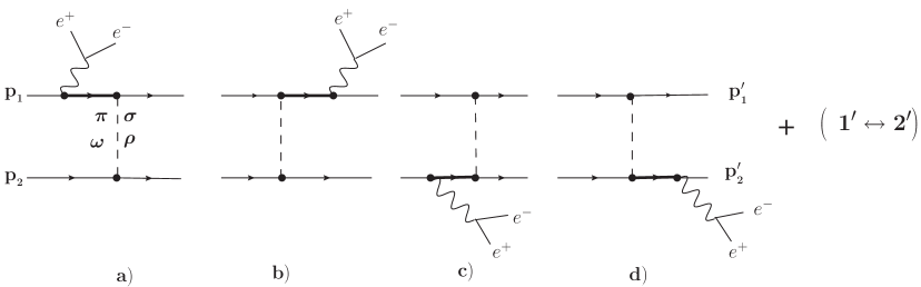
Figure 1: Bremsstrahlung diagrams for the process $N_{1}+N_{2}\to N_{1}^{\prime}+N_{2}^{\prime}+e^{+}+e^{-}$. Fat lines are for resonances considered in section III.

The form of the cross section Eq. (7) exploits essentially the gauge invariance of hadronic and leptonic tensors. This implies that in elaborating models for the reaction (1) with effective Lagrangians, particular attention must be devoted to the gauge invariance of the computed currents with the mandatory condition $q_{\mu}J^{\mu}=0$. In our approach, i.e., in the one-boson exchange approximation (OBE) for the strong $NN$ interaction and one-photon exchange for the electromagnetic production of $e^{+}e^{-}$, the current $J_{\mu}$ is determined by diagrams of two types: (i) the ones which describe the creation of a virtual photon with $q^{2}>0$ as pure nucleon bremsstrahlung as depicted in Fig. 1 and (ii) in case of exchange of charged mesons, the emission of a virtual photon ($\gamma^{*}$) from internal meson lines, see Fig. 2a. For these diagrams the gauge invariance is tightly connected with the two-body Ward-Takahashi (WT) identity

$$q_{\mu}\Gamma^{\mu}(p^{\prime},p)=\frac{e(1+\tau_{3})}{2}\left(S^{-1}(p^{\prime})-S^{-1}(p)\right),$$ (12)

where $\Gamma^{\mu}$ denotes the electromagnetic vertex and $S(p)$ is the (full) propagator of the respective particle. It is straightforward to show that, if (12) is to be fulfilled, then pairwise two diagrams with exchange of neutral mesons and pre-emission and post-emission of $\gamma^{*}$ (cf.  Figs. 1a) and b)) cancel each other, hence ensuring $q^{\mu}J_{\mu}=0$, i.e., current conservation. This is also true after dressing the vertices with phenomenological form factors. However, in case of charged meson exchange the WT identity is not any more automatically fulfilled. This is because the nucleon momenta are interchanged and, consequently, the ”right” and ”left” internal nucleon propagators are defined for different momenta of the exchanged meson.

In order to restore the gauge invariance on this level one must consider additional diagrams with emission of the virtual photon by the charged meson exchange (Fig. 2a) which exactly compensates the non-zero part of the current divergence, and thus gauge invariance is restored. This holds true for bar $NNM$ vertices without cut-off form factors. Inclusion of additional form factors again leads to non-conserved currents. There are several prescriptions of how to preserve gauge invariance within effective theories with cut-off form factors.

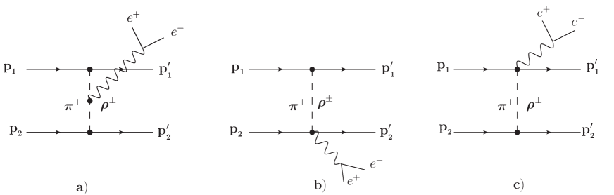
Figure 2: Contribution of meson exchange currents (a) and seagull terms (b, c) to the process $N_{1}+N_{2}\to N_{1}^{\prime}+N_{2}^{\prime}+e^{+}e^{-}$, where $N_{1}$ and $N_{2}^{\prime}$ stand for protons and $N_{2}$ and $N_{1}^{\prime}$ denote neutrons.

The main idea of these prescriptions is to consider the cut-off form factors as phenomenological part of the self-energy corrections to the corresponding propagators; the full propagators are to be treated as the bare ones multiplied at both ends by a form factor gross . Then, the full propagator, e.g. for mesons, can be defined as

$$\Delta(k)=\frac{1}{k^{2}-\mu_{M}^{2}+\Pi(k)}\equiv\frac{F_{M}^{2}(k)}{k^{2}-\mu_{M}^{2}},$$ (13)

where $\Pi(k)$ is the self-energy correction (see Fig. 3).

Figure 3: Graphical illustration of the cut-off form factor as self-energy corrections to the full propagator gross .

In the simplest case, for mesonic vertices with pseudoscalar couplings, the bare mesonic vertex $\Gamma_{\mu}^{M}=\left(k_{1\mu}+k_{2\mu}\right)$ receives an additional factor schafer ; mathiot ; ourbrem becoming

$$\Gamma_{\mu}^{\gamma M}=\left(k_{1\mu}+k_{2\mu}\right)\frac{\left(\Lambda_{M}^{2}-k_{1}^{2}\right)}{\left(\Lambda_{M}^{2}-\mu_{M}^{2}\right)}\frac{\left(\Lambda_{M}^{2}-k_{2}^{2}\right)}{\left(\Lambda_{M}^{2}-\mu_{M}^{2}\right)}\left(1-\frac{k_{1}^{2}-\mu_{M}^{2}}{\Lambda_{m}^{2}-k_{2}^{2}}-\frac{k_{2}^{2}-\mu_{M}^{2}}{\Lambda_{M}^{2}-k_{1}^{2}}\right).$$ (14)

The above prescriptions for restoration of the gauge invariance in $pn$ collisions are valid only for pion exchange diagrams with the interaction vertices independent of the momentum $k$ of the exchanged meson, i.e., solely for the case of pseudo-scalar $\pi NN$ coupling. The presence of field derivatives in the interaction Lagrangian, e.g. the case for pseudo-vector $\pi NN$ coupling or for vector mesons, Eqs. (9) and (10), requires a more refined treatment of the gauge invariance. In the simplest case, besides the WT identity condition (with full propagators) for the diagram 2a, the gauge invariance requires an introduction of covariant derivatives, i.e. the replacement of the partial derivatives, including the $NNM$ vertices, by a covariant form (minimal coupling). Such a procedure generates another kind of Feynman diagrams with contact terms, i.e., vertices with four lines, known also as Kroll-Rudermann KR or seagull like diagrams, see Figs. 2b and c. We include therefore in our calculations these diagrams by the corresponding interaction Lagrangian

$${\cal L}_{NN\pi\gamma}=-\frac{\hat{e}f_{NN\pi}}{m_{\pi}}\bar{N}\gamma_{5}\gamma^{\mu}A_{\mu}({{\mathchar 28956\relax}{\mathchar 28680\relax}_{(\pi)}})N$$ (15)

with electromagnetic four-potential $A_{\mu}$ and charge operator $\hat{e}$ of the pion. Analogously for the $\rho NN$ coupling one has to replace

$$\frac{\kappa_{\rho}}{2m}\bar{N}\sigma_{\mu\nu}{{\mathchar 28956\relax}}N\partial^{\nu}{\mathchar 28680\relax}_{(\rho)}^{\mu}\,\longrightarrow\,\frac{\kappa_{\rho}}{2m}\bar{N}\sigma_{\mu\nu}{{\mathchar 28956\relax}}N\partial^{\nu}{\mathchar 28680\relax}_{(\rho)}^{\mu}+\hat{e}\frac{\kappa_{\rho}}{2m}\bar{N}\sigma_{\mu\nu}{{\mathchar 28956\relax}}NA_{\nu}{\mathchar 28680\relax}_{(\rho)}^{\mu}.$$ (16)

Gauge invariance is henceforth ensured. It should be stressed that as far as the tensor part of the $\rho NN$ Lagrangian (see Eq. (10)) is accounted for, the prescription (16) must be mandatorily applied, regardless of the choice of $\pi NN$ coupling. This implies that calculations with pseudo-scalar couplings for the pion-nucleon vertex violates gauge invariance due to $\rho$ meson exchange. Our numerical calculations show that the effect of such $\rho$ exchange seagull type diagrams vary from $10\%$ at low di-electron invariant masses up to 35% at the kinematical limit.

All electromagnetic $NN\gamma$ vertices correspond to the interaction Lagrangian

$${\cal L}^{em}_{NN\gamma}=-e\left(\bar{N}\gamma_{\mu}N\right)A^{\mu}+e\kappa\bar{N}\left(\frac{\sigma_{\mu\nu}}{4m}{\cal F}^{\mu\nu}\right)N$$ (17)

with the field strength tensor ${\cal F}_{\mu\nu}=\partial_{\nu}A_{\mu}-\partial_{\mu}A_{\nu}$, and $\kappa$ as the anomalous magnetic moment of the nucleon ($\kappa=1.793$ for protons and $\kappa=-1.913$ for neutrons).

II.5 Results for bremsstrahlung

The OBE parameters and their energy dependence have been taken as in Ref. ourbrem ; mosel_calc . Figure 4 exhibits results of our calculations of the invariant-mass distribution of di-electrons in $pp$ and $pn$ collisions from bremsstrahlung processes in Figs. 1 and 2 (nucleons only) at two values of the kinetic energy, 1.04 GeV and 1.25 GeV as relevant for DLS DLS and HADES HADES1 measurements. In our actual calculations we include, besides the mentioned four exchange mesons $\pi$, $\sigma$, $\rho$ and $\omega$ also a ”counter term” simulating a heavy axial vector-isovector meson, with the goal to cancel singularities of the pion potential at the origin mosel_calc . The dotted lines in Fig. 4 depict the cross section in $pn$ collision, while the solid lines stand for results of $pp$ reactions. It is seen that the $pn$ cross section is by a factor $5-6$ larger than the $pp$ cross section. (The situation for real photon emission is similar: The $pn$ channel has a significant contribution, while, due to a destructive interference, the $pp$ channel is much weaker and is often neglected barz .) This is due to isospin effects for the charged $\pi$ and $\rho$ mesons and different interference effects in $pp$ and $pn$ channels. In $pn$ reactions, additional contributions stem from the emission off charged exchange mesons and from corresponding seagull type diagrams. Note that in both channels, $pp$ and $pn$, numerical tests of gauge invariance can serve as additional check of the code. The meson exchange diagrams together with contact terms amplify the contribution of pure nucleonic currents; their contribution is of the order of $\sim 40\%$ at low values of the invariant di-electron masses and increases up to a factor $2-3$ at higher invariant masses.

Figure 4: Contribution of the bremsstrahlung diagrams in Figs. 1 and 2 (without nucleon resonances) to the $e^{+}e^{-}$ invariant mass distribution at two kinetic energies (left: 1.04 GeV, right: 1.25 GeV). Solid lines correspond to $pp$ reactions; dashed lines are for $pn$ reactions.

III resonances

Intermediate baryon resonances play an important role in di-electron production in $NN$ collisions at beam energies in the 1 - 2 GeV region fuchs ; ernst ; nakayama ; lutzNew ; kapusta ; mosel_calc ; ikh_model ; schafer ; brat . The main contribution to the cross section stems from the $\Delta$ isobar mosel_calc . Also, the low-lying nucleon resonances such as $N^{*}(1440)$, $N^{*}(1520)$ and $N^{*}({1535})$ contribute to the cross section. We are going to investigate separately each of these resonances represented in Fig. 1 by fat lines.

III.1 $P_{33}(1232)$

Since the isospin of the $\Delta$ is $3/2$ only the isovector mesons $\pi$ and $\rho$ couple to nucleons and $\Delta$’s. The form of the effective $\Delta N$ interaction was thoroughly investigated in literature in connection with $NN$ scattering bonncd ; holinde ; weise , pion photo- and electroproduction pascQuant ; photo ; davidson ; elctro ; lenske . The effective Lagrangians of the $\Delta NM$ interactions read holinde ; weise ; pascQuant

$${\cal L}_{\Delta N\pi}=\frac{f_{\Delta N\pi}}{m_{\pi}}\left(\bar{\Psi}_{\Delta}^{\alpha}\ {\bf T}\ \partial_{\alpha}{\mathchar 28680\relax}_{(\pi)}N\right)+h.c.,$$ (18)

$${\cal L}_{\Delta N\rho}=\frac{if_{\Delta N\rho}}{m_{\rho}}\left(\bar{\Psi}_{\Delta\,\alpha}{\bf T}\left\{\partial^{\beta}{\mathchar 28680\relax}_{(\rho)}^{\alpha}-\partial^{\alpha}{\mathchar 28680\relax}_{(\rho)}^{\beta}\right\}\gamma_{\beta}\gamma_{5}N\right)+h.c.$$ (19)

with $f_{\Delta N\pi}=2.13$ GeV and $f_{\Delta N\rho}=7.14$ GeV schafer . The $\Delta NM$ vertices are dressed by cut-off form factors

$$F^{\Delta NM}=\left[\frac{\Lambda_{\Delta NM}^{2}-\mu_{M}^{2}}{\Lambda_{\Delta NM}^{2}-k^{2}}\right]^{2},$$ (20)

where $\Lambda_{\Delta N\pi}=1.4214$ GeV and $\Lambda_{\Delta N\rho}=2.273$ GeV schafer . The symbol ${\bf T}$ in Eqs. (18) and (19) stands for the isospin transition matrix, and $\Psi_{\Delta}$ denotes the field describing the $\Delta$. Particles with higher spins ($s>1$) are treated usually within the Rarita-Schwinger formalism in accordance with which the $\Delta$ propagator has the form

$$S_{\Delta}^{\alpha\beta}(p,m_{\Delta})=\frac{i\left(\hat{p}+m_{\Delta}\right)}{p^{2}-m_{\Delta}^{2}}\ P_{\frac{3}{2}}^{\alpha\beta}(p,m_{\Delta})$$ (21)

with the spin projection operator $P_{\frac{3}{2}}^{\alpha\beta}(p)$ defined as

$$P_{\frac{3}{2}}^{\alpha\beta}(p,m_{\Delta})=-g^{\alpha\beta}+\frac{1}{3}\gamma^{\alpha}\gamma^{\beta}+\frac{2}{3m_{\Delta}^{2}}p^{\alpha}p^{\beta}+\frac{1}{3m_{\Delta}}\left(\gamma^{\alpha}p^{\beta}-\gamma^{\beta}p^{\alpha}\right).$$ (22)

In addition, to take into account the widths of $\Delta$, the mass in the denominator of the scalar part of the propagator is modified as $m_{\Delta}\to m_{\Delta}-i\Gamma_{\Delta}/2$. For the kinematics considered here, the ”mass” $\sqrt{p^{2}}$ of the intermediate $\Delta$ can be rather far from its pole value. The width, as a function of $p^{2}$, is calculated as a sum of partial widths being dominated by the one-pion ($\Delta\to N\pi$) and two-pion ($\Delta\to N\rho\to N\pi\pi$) decay channels shyamwidts .

The general form of the $\Delta N\gamma$ coupling satisfying gauge invariance can be written as davidson ; feuster ; pascTjon ; pascScholten

$${\cal L}_{\Delta N\gamma} = -i\frac{eg_{1}}{2m}\bar{\Psi}^{\alpha}\Theta_{\alpha\mu}(z_{1})\gamma_{\nu}\gamma_{5}{\bf T}_{3}N{\cal F}^{\nu\mu}-\frac{eg_{2}}{4m^{2}}\bar{\Psi}^{\alpha}\Theta_{\alpha\mu}(z_{2})\gamma_{5}{\bf T}_{3}\left(\partial_{\nu}N\right){\cal F}^{\nu\mu}$$ (23)

$$-\frac{eg_{3}}{4m^{2}}\bar{\Psi}^{\alpha}\Theta_{\alpha\mu}(z_{3})\gamma_{5}{\bf T}_{3}N\partial_{\nu}{\cal F}^{\nu\mu}+h.c.,$$

$$\Theta_{\alpha\mu}(z) = g_{\alpha\mu}+[z+\frac{1}{2}(1+4z)A]\gamma_{\alpha}\gamma_{\mu},$$ (24)

where $A$ is a constant reflecting the invariance of the free $\Delta$ Lagrangian with respect to point transformations which, according to common practice, is taken $A=-1$. The other parameters, $z_{1},z_{2}$ and $z_{3}$ are also connected with point transformations; however, they characterize the off-mass shell $\Delta$ resonance and remain unconstrained. The two coupling constants $g_{1}$ and $g_{2}$ in Eq. (23) can be estimated from experimental data with real photons ($q^{2}=0$) by evaluating the helicity amplitudes helicity of the process $\Delta\to\gamma N$ obtained within the Lagrangian Eq. (23). One finds explicitly

$$eg_{1}\left\langle{\bf T}_{3}\right\rangle=-2\sqrt{2}\frac{m}{m+m_{\Delta}}\sqrt{\frac{m_{\Delta}m}{|{\bf q}^{*}|}}\left[\sqrt{3}A_{\frac{1}{2}}^{PDG}+A_{\frac{3}{2}}^{PDG}\right],$$ (25)

$$eg_{2}\left\langle{\bf T}_{3}\right\rangle=-4\sqrt{2}\left(\frac{m}{m_{\Delta}|{\bf q}^{*}|}\right)^{\frac{3}{2}}mm_{\Delta}\left[\sqrt{3}A_{\frac{1}{2}}^{PDG}-\frac{m}{m_{\Delta}}A_{\frac{3}{2}}^{PDG}\right],$$ (26)

where $|{\bf q}^{*}|$ is the three-momentum of the photon in the $\Delta$ center-of-mass system, and the helicity amplitudes $A_{\frac{1}{2}(\frac{3}{2})}^{PDG}$ are normalized in such a way that they correspond to values listed by Particle Data Group (PDG) PDG . It should be pointed out that both coupling constants $g_{1,2}$ are quite sensitive to the values of the helicity amplitudes, which, according to PDG, vary in rather large intervals: $-A_{\frac{1}{2}}^{PDG}\sim 0.128\cdots 0.145$, $-A_{\frac{3}{2}}^{PDG}\sim 0.243\cdots 0.261$, PDG providing the uncertainties $g_{1}\sim 4.5\cdots 5.5$ and $g_{2}\sim 4.5\cdots 8.5$. In principle, the computed electromagnetic width of $\Delta$ can serve as an additional constraint for the coupling constants. However it turns out that it is less sensitive to the actual choice of $g_{1,2}$ yielding satisfactorily good results for different sets of $g_{1,2}$ obtained from helicity amplitudes. Another uncertainty ($\sim 20\%$) in Eqs. (25) and (26) follows from the normalization of the isospin transition matrix $\left\langle{\bf T}_{3}\right\rangle$ which can be chosen either $\sqrt{\frac{2}{3}}$ or $1$ (see discussion appendix A in ourbrem ). The remaining constants in Eq. (23), $z_{1,2,3}$ and $g_{3}$, do not contribute in processes with on-mass shell particles and cannot be directly related to data. As a matter of fact, they are considered as free fitting parameters feuster . In the present calculation we use $g_{1}=5.478$, $z_{1}=0.05$, $g_{2}=7.611$, $z_{2}=1.499$, $g_{3}=7.0$ and $z_{3}=0$ being consistent with the available experimental data on helicity amplitudes, electromagnetic decay width and pion photoproduction (cf. Ref. feuster ).

Figure 5: Invariant mass distribution of $e^{+}e^{-}$ pairs in proton-proton (upper row) and proton-neutron (lower row) collisions. The dashed (dotted) curves depict the contribution of diagrams with bremsstrahlung from $\gamma\Delta N$ ($\gamma NN$) vertices. In $pn$ channels, the meson exchange and seagull type diagram are accounted for as well. The solid lines are the results of calculations of the cross section as coherent sum of all nucleon and $\Delta$ contributions.

With these parameters we calculate the invariant mass distribution of di-electrons produced in $pp$ and $pn$ collisions. Figure 5 exhibits the mass distribution at two values of the kinetic energy, $1.04$ and $1.25$ GeV. The dotted lines depict the contribution from pure bremsstrahlung processes from the nucleon lines including meson exchange and seagull diagrams for $pn$ reactions (cf. Fig. 4), while the dashed lines are the contributions of the $\Delta$. The solid lines exhibit the coherent sum of nucleon and $\Delta$ contributions. The normalization of the isospin transition matrix has been chosen as 1. It can be seen that the $\Delta$ contribution dominates in the whole kinematic range , except for the region near the kinematical limit, where the nucleon current contributions become comparable with $\Delta$ contributions. It should be noted that, since at considered energies the off-mass shellness of $\Delta$ is not large, the contribution of off-mass shell parameters $z_{i}$ is rather small, except in the region near the kinematical limits where the behavior of the cross section is slightly modified. However, since the electromagnetic coupling constants $g_{i}$ have been adjusted to experimental data together with off-mass shell parameters feuster , we keep $z_{i}$ as in Ref. feuster for the sake of consistency. Also note that the coupling constants $g_{1,2}$ have been fixed at the photon point, i.e., at $q^{2}=0$, while in our case the virtual photon is massive. In principle, one may introduce a $q^{2}$ dependence of the coupling strengths in form of some phenomenological form factors which avoid an unphysical behavior at large virtuality of $\Delta$, i.e., at large $q^{2}$.

To have an estimate of the role of these parameters for off-mass shell $\Delta$’s, it is instructive to investigate the invariant mass distribution in the Dalitz decay of an off-mass shell particle with all quantum numbers as the $\Delta$ but with different mass $p^{2}\neq m_{\Delta}^{2}$. Such a quantity is often used in two-step models when calculating di-electrons from $NN$ collisions brat08 ; ernst ; ikh_model , where in a first step a $\Delta$ like particle is created, then in the second step it decays into a nucleon and a di-electron. There are essentially two options for a treatment of such a process:
(1) Everything is on-mass shell, i.e. in the $\Delta$ Lagrangian, and in the positive energy projector operators $(\hat{p}+m_{\Delta})$, Eq. (21), and in the spin projection operator $P_{\frac{3}{2}}(p,m_{\Delta})$, Eq. (22), one takes the mass parameter as $m_{\Delta}\Rightarrow m_{X}$. This means that the produced on-mass shell particle with a mass $m_{X}\neq m_{\Delta}$ is nevertheless described by a $\Delta$ Lagrangian with the same coupling constants. This leads merely to a shift in masses in the expression for the invariant mass distribution and to a corresponding enlargement of the phase space volume. Evidently, since in this case $p^{2}=m_{X}^{2}$ and due to the relation $\gamma_{\alpha}(\hat{p}+m_{X})P_{\frac{3}{2}}^{\alpha\beta}(p,m_{X})=(\hat{p}+m_{X})P_{\frac{3}{2}}^{\alpha\beta}(p,m_{X})\ \gamma_{\alpha}=0$, the dependence on $z_{i}$ drops out in such a treatment (see Eq. (24)).
(2) The $\Delta$ is considered off-mass shell, i.e., in the Lagrangian and projection operators (22) and (21) one keeps the mass parameter as $m_{\Delta}$, while $p^{2}\neq m_{\Delta}^{2}$ (see ernst ). In this case the positive energy projection operator $(\hat{p}+m_{\Delta})$ does not commute with the spin projection operator $P_{\frac{3}{2}}(p,m_{\Delta})$ causing problems in the treatment of the Rarita-Schwinger propagator for off-mass shell particles (see discussion in Ref. ourbrem ). Obviously, the off-mass shell parameters $z_{i}$ can now contribute. The mass distribution of the Dalitz decay with $p^{2}\neq m_{\Delta}^{2}$ but with $P_{\frac{3}{2}}(p,m_{\Delta})$ is called the ”off-mass shell” Dalitz decay.

By using Eq. (6), the invariant-mass distribution from the decay of a $\Delta$-like particle into a $e^{+}e^{-}$ pair with invariant mass $M$ can be presented in the following form:

$$\frac{d\Gamma^{\Delta_{x}\to Ne^{+}e^{-}}}{dM}=-\frac{\alpha^{2}_{em}}{12\pi}\frac{|{\bf p}_{N}|}{m_{X}^{2}}\frac{1}{M}K_{\mu}\ K^{+\mu},$$ (27)

where $|{\bf p}_{N}|$ is the momentum of the outgoing nucleon in the $\Delta$ center of mass system, and the amplitude of a virtual photon production $\Delta_{X}\to N\gamma^{*}$ is defined as

$$K_{\mu}\ K^{+\mu}={\rm Tr}\left[(\hat{p}_{N}+m)\ {G^{\mu,}}_{\alpha}\ (\hat{p}+m_{X})P_{\frac{3}{2}}^{\alpha\beta}(p,m_{X})\bar{G}_{\mu,\beta}\right]$$ (28)

with

$$G^{\mu,\alpha}=-\left[\frac{g_{1}}{2m}\gamma^{\nu}\Theta^{\mu^{\prime}\alpha}(z_{1})+\frac{g_{2}}{4m^{2}}p_{N}^{\nu}\Theta^{\mu^{\prime}\alpha}(z_{2})+\frac{g_{3}}{4m^{2}}q^{\nu}\Theta^{\mu^{\prime}\alpha}(z_{3})\right]\left[\phantom{\frac{1}{2}}\!\!q_{\mu^{\prime}}g^{\mu}_{\nu}-q_{\nu}g^{\mu}_{\mu^{\prime}}\right]\gamma_{5}.$$ (29)

In Fig. 6 (left panel), the mass distribution (27) is presented for the case of on-mass shell $\Delta$-like particles. It can be seen that due to larger phase space volume, the mass distribution of heavier particles is much larger than the distribution for real on-mass shell $\Delta$.

Figure 6: Invariant mass distribution according to Eq. (27) for the decay of a $\Delta$-like particle $m_{X}\rightarrow Ne^{+}e^{-}$. Left panel: the mass parameters $m_{X}=1.232$ GeV (lower curves) and at $m_{X}=1.850$ GeV (upper curves) are taken on-mass shell, i.e., case (1) with $p^{2}=m_{X}^{2}$. The solid and dashed lines correspond to isospin normalization $\left\langle{\bf T}_{3}\right\rangle$ to 1 and to $\sqrt{\frac{2}{3}}$, respectively. Right panel: The on-mass shell mass distribution (solid line) versus off-mass shell calculations in case (2), i.e., with the spin projection operator $P_{\frac{3}{2}}(p,m_{X})$, Eq. (22), and the electromagnetic vertices Eq. (29) calculated at $p^{2}\neq m_{\Delta}^{2}$ (dashed line). In all calculations the coupling constants in Eq. (29) are $g_{1}=5.478$, $g_{2}=7.611$ and $g_{3}=7.0$. For the right panel the off-mass shell parameters have been taken as $z_{i}=-0.5$.

In Fig. 6 (right panel), a comparison of results of calculations of the off mass shell distribution are presented for $m_{X}=1.85$ GeV. The solid line is for the ”on-mass shell” case (1), while the off-mass shell results for case (2) are presented by dashed lines. It can be seen that the off-mass shell calculations considerably differ from the commonly accepted results with $\Delta$ on-mass shell. This demonstrates that in two-step models, besides the traditional approximations, there are additional uncertainties in the treatment the Dalitz decay of the off-mass shell $\Delta$ at large values of invariant mass. It is clear that, if in two-step models off-mass shell calculations are employed, additional form factors must be considered to suppress such an increase of the mass distribution at large virtuality of the decaying $\Delta$.

III.2 Spin-$\frac{1}{2}$ resonances $P_{11}(1440)$ and $S_{11}(1535)$

Contrarily to the $\Delta$ isobars, the isospin-$\frac{1}{2}$ nucleon resonances can couple not only with isospin-1 mesons, but also $\sigma$, $\eta$ and $\omega$ mesons may contribute. The corresponding Lagragians are

$${\cal L}_{NN^{*}ps}^{(\pm)} = \mp\frac{g_{NN^{*}ps}}{m_{N^{*}}\pm m}\bar{\Psi}_{N^{*}}\left\{\begin{array}[]{c}\gamma_{5}\\ 1\end{array}\right\}\gamma_{\mu}(\partial^{\mu}\Phi_{(ps)})N+h.c.,$$ (32)

$${\cal L}_{NN^{*}V}^{(\pm)} = \frac{g_{NN^{*}V}}{2(m_{N^{*}}+m)}\bar{\Psi}_{N^{*}}(x)\left\{\begin{array}[]{c}1\\ \gamma_{5}\end{array}\right\}\sigma_{\mu\nu}V^{\mu\nu}(x)N+h.c.,$$ (35)

$${\cal L}_{NN^{*}\sigma}^{(\pm)} = -g_{NN^{*}\sigma}\bar{\Psi}_{N^{*}}\left\{\begin{array}[]{c}1\\ \gamma_{5}\end{array}\right\}N\it\Phi_{(\sigma)}+h.c.$$ (38)

with the abbreviations $ps\equiv\pi$ or $\eta$, $\Phi_{(ps)}\equiv({\mathchar 28956\relax}{\mathchar 28680\relax}_{(\pi)})$ or $\Phi_{(\eta)}(x)$, $V\equiv V_{(\omega)}$ or $V({\mathchar 28956\relax}{\mathchar 28954\relax})$, and $V^{\alpha\beta}=\partial^{\beta}V^{\alpha}-\partial^{\alpha}V^{\beta}$. (The additionally introduced $\eta$ exchange employs for the $NN\eta$ interaction ${\cal L}_{NN\eta}=-\frac{f_{NN\eta}}{m_{\eta}}\bar{N}\gamma_{5}\gamma^{\mu}(\partial_{\mu}\Phi_{(\eta)})N$ with $f_{NN\eta}=1.79$ from Ref. bonncd .) At a first glance, the consideration of Lagrangians (32)-(38) involves into the calculations additional free parameters. However, the effective constants are not completely free and indeed they can be estimated from independent experimental data. The coupling constants of the resonances with the pseudo-scalar meson can be found from the calculations of the experimentally known PDG partial width of the corresponding decay

$$\Gamma_{N^{*}\to Nps}^{\pm}=g_{NN^{*}ps}^{2}\frac{{\cal I}}{8\pi}\frac{|{\bf p^{*}}|}{m_{N^{*}}^{2}}\left[\left(m_{N^{*}}\mp m\right)^{2}-m_{\pi}^{2}\right],$$ (39)

where ${\cal I}=3$ for pions and ${\cal I}=1$ otherwise. This yields $g_{NN^{*}\pi}^{2}=6.54$, $g_{NN^{*}\eta}^{2}=0.5$ for the Roper resonance $N(1440)$ and $g_{NN^{*}\pi}^{2}=1.25$, $g_{NN^{*}\eta}^{2}=2.02$ for the $N(1535)$ resonance.

Estimates of coupling constants with $\sigma$ mesons, for which direct experimental data are not available, are more involved. One of the method is to calculate the decay of the considered resonances into two pions in a specific final state, $N(2\pi)^{I=0}_{S=0}$. For low-lying resonances such a decay can be treated as a process with intermediate excitation of the $\sigma$ meson with its subsequent decay into two pions soyer2pi , as depicted in Fig. 7.

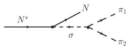
Figure 7: Diagram for the decay of a resonance $N^{*}$ in to two pions in the state $S=0$, $I=0$ with an intermediate $\sigma$ meson.

A direct calculation of the diagram Fig. 7 results in

$$\!\!\!\!\!\!\!\!\!\Gamma_{N^{*}\to N(2\pi)^{I=0}_{S=0}}^{\pm}=\frac{g_{NN^{*}\sigma}^{2}}{4\pi}\int\limits_{2m_{\pi}}^{m_{N^{*}}-m}d\xi\frac{|{\bf p^{*}}|m_{\sigma}^{2}\left[(m_{N^{*}}\pm m)^{2}-\xi^{2}\right]}{|\xi^{2}-(m_{\sigma}-\frac{i}{2}\Gamma)^{2}|^{2}}\frac{\Gamma_{\sigma\to 2\pi}}{\pi\ m_{N^{*}}^{2}}\sqrt{\frac{\xi^{2}-4m_{\pi}^{2}}{m_{\sigma}^{2}-4m_{\pi}^{2}}},$$ (40)

where the dependence of the width $\sigma\to 2\pi$ on the mass $\xi$ of the intermediate meson is computed from the Lagrangian

$${\cal L}_{\sigma\pi\pi}=g_{\sigma\pi\pi}\frac{m_{\sigma}}{2}\left({\mathchar 28680\relax}_{(\pi)}{\mathchar 28680\relax}_{(\pi)}\right)\Phi_{(\sigma)}$$ (41)

with the coupling constant $g_{\sigma\pi\pi}$ found from the total decay width of the $\sigma$ meson into two pions. In the present calculation we adopt $m_{\sigma}=500$ MeV and $\Gamma_{\sigma\to 2\pi}=250$ MeV being consistent with the recent analysis leutw . With these parameters we obtain $g_{NN^{*}\sigma}=2.1$ for the Roper resonance and $g_{NN^{*}\sigma}=3.8$ for $N(1535)$ (see also nakayamac69 ). The propagator of the off-mass shell resonance, $p_{X}^{2}\neq m_{N^{*}}^{2}$, is augmented by a form factor of the form

$$F(p_{X})=\frac{\Lambda^{4}}{\Lambda^{4}+(p_{X}^{2}-m_{N^{*}}^{2})^{2}}$$ (42)

with $\Lambda=1.2$ GeV in both cases, for Roper and $N(1535)$ resonances. The finite widths of the intermediate resonances are taken into account as usually: adding to the mass parameter in the propagator an imaginary part as $m_{N^{*}}\to m_{N^{*}}-i\Gamma^{tot}/2$. In our case, the resonances are off mass shell and their total widths depend on the invariant masses of the resonance. Such a dependence can be parameterized as feuster

$$\Gamma^{tot}(m_{X})=\sum_{i}\Gamma_{i}(m_{X})F_{X}(m_{X}),$$ (43)

where the sum runs over all possible partial decay channels, and the cut-off form factors $F_{X}(m_{X})$ suppress an unphysical increase of the width with increasing $m_{X}$.

$$F_{X}(m_{X})=\frac{2}{1+\left(\frac{P^{*}(m_{X})}{P^{*}(m_{N^{*}})}\right)^{\alpha}},$$ (44)

where $P^{*}$ is the nucleon momentum in the resonance center of mass system, $\alpha=3$ and $\alpha=2$ for the Roper and $N(1535)$ resonances, respectively. For the Roper resonance there are two main decay channels, $N(1440)\to N\pi$ (branching ratio $\sim 60-70\%$) and $N(1440)\to\Delta\pi$ (branching ratio $\sim 20-30\%$) PDG , while $N(1535)$ decays mainly either into a nucleon and a pion (branching ratio $\sim 55\%$) or into a nucleon and $\eta$ (branching ratio $\sim 45\%$). The energy dependence of the partial widths $\Gamma_{i}(m_{X})$ for two-body decay have been calculated using the same Lagrangians (32)-(38). For the decay of the Roper resonance $N^{*}\to N\pi\pi$ via $\Delta$ we employ an effective Lagrangian of the form

$${\cal L}_{N^{*}\Delta\pi}=\frac{f_{N^{*}\Delta\pi}}{m_{\pi}}\bar{\Psi}^{\alpha}{\bf T}\partial_{\alpha}{\mathchar 28680\relax}_{(\pi)}N^{*}+h.c..$$ (45)

Note that by calculating the energy dependence of the widths from the Lagrangian (45) a knowledge of the coupling constant $f_{N^{*}\Delta\pi}$ is not necessary. Also note that, in spite of the mass of the Roper resonance which is only slightly above the kinematical limit, the probability to decay into $\Delta$ and $\pi$ is relatively large. This is due to the large total width of the $\Delta$ resonance which correspondingly spreads the mass around the pole position, enlarging therefore the phase space of the decay channel. In calculating the partial width $N^{*}\to\pi\Delta$ we adopt a Gaussian distribution of the mass of the $\Delta$ resonance $f(\tilde{m}_{\Delta})=(\sigma_{\Delta}\sqrt{2\pi})^{-1}\exp[-(\tilde{m}_{\Delta}-m_{\Delta})^{2}/(2\sigma_{\Delta}^{2})]$ with $\sigma_{\Delta}=\Gamma_{\Delta}$. The remaining coupling constants for the vector mesons have been taken from Ref. nakayamac69 (see Tab. 1) .

Table 1: Coupling constants $g_{NN^{*}M}$ and cut-off parameters $\Lambda$ for the effective Lagrangians (32)-(38), computed either directly from the decay widths or taken from Ref. nakayamac69 .

Meson		$P_{11}(1440)$		$S_{11}(1535)$		$\Lambda$ [GeV]
$\pi$		6.54		1.25		1.2
$\eta$		0.5		2.02		1.2
$\sigma$		2.1		3.8		1.2
$\rho$		-0.57		- 0.65		1.2
$\omega$		- 0.37		-0.72		1.2

The effective Lagrangian for the electromagnetic decay of the resonance into a photon and a nucleon has been taken as

$${\cal L}_{NN^{*}\gamma}^{\pm}=\frac{e\kappa}{2m_{R}}\bar{\Psi}_{N^{*}}\left\{\begin{array}[]{c}1\\ \gamma_{5}\end{array}\right\}\sigma^{\mu\nu}NF_{\mu\nu}+h.c.,$$ (48)

where, in contrast to the $\Delta$ case, the coupling $\kappa$ is different for proton and neutron vertices and can be found from the helicity amplitudes

$$A_{1/2}=-{e\kappa}\ \sqrt{\frac{|{\bf p^{*}}|}{mm_{N^{*}}}},$$ (49)

where for the Roper resonance one has $A_{1/2}^{p}=-0.065\ \rm GeV^{-1/2}$ and $A_{1/2}^{n}=0.04\ \rm GeV^{-1/2}$, while for the $N(1535)$ we employ $A_{1/2}^{p}=0.09\ \rm GeV^{-1/2}$ and $A_{1/2}^{n}=-0.046\ \rm GeV^{-1/2}$, correspondingly.

III.3 Spin-$\frac{3}{2}$ nucleon resonances

The next considered resonance is $D_{13}(1520)$ with negative parity and spin $\frac{3}{2}$. The effective Lagrangian for such resonances is chosen in the same form as for the $\Delta$ with the exception that, since the isospin is $\frac{1}{2}$, besides the isovector mesons $\pi$ and $\rho$, the isoscalar $\eta$, $\omega$ and $\sigma$ also can contribute. The effective Lagrangians are as follows

$${\cal L}_{NN^{*}ps}^{(\pm)} = \frac{g_{NN^{*}ps}}{m_{ps}}\bar{\Psi}_{N^{*}}^{\alpha}(x)\left\{\begin{array}[]{c}1\\ \gamma_{5}\end{array}\right\}(\partial_{\alpha}\Phi_{(ps)})N+h.c.,$$ (52)

$${\cal L}_{NN^{*}V}^{(\pm)} = \mp i\frac{g_{NN^{*}V}}{m_{V}}\bar{\Psi}_{N^{*}}^{\alpha}\left\{\begin{array}[]{c}\gamma_{5}\\ 1\end{array}\right\}\gamma^{\lambda}V_{\alpha\lambda}N+h.c.,$$ (55)

$${\cal L}_{NN^{*}\sigma}^{(\pm)} = i\frac{g_{NN^{*}\sigma}}{m_{\sigma}}\bar{\Psi}_{N^{*}}^{\alpha}\left\{\begin{array}[]{c}\gamma_{5}\\ 1\end{array}\right\}(\partial_{\alpha}\Phi_{(\sigma)})N+h.c..$$ (58)

Note that in choosing the relative phase for the $\sigma$ meson an imaginary unit $i$ must be explicitly displayed. In principle, to synchronize the relative phases of different Lagrangians one may compute the corresponding amplitude in a fully coplanar kinematics. Then such an amplitude, in tree level calculations, must be either purely real or purely imaginary. The coupling constants and the cut-off parameter $\Lambda=0.8$ GeV have been taken from Ref. mosel_calc . The propagator is chosen in the form (21) with the resonance mass augmented by the total decay width. The total width of the resonance $N(1520)$ is calculated by Eq. (43) for which three decay channels have been taken into account, $N(1520)\to N\pi$ (branching ratio $\sim$ 50%), $N(1520)\to N\rho$ (branching ratio $\sim$ 25%) and $N(1520)\to N\Delta$ (branching ratio $\sim$ 25%). For the decay in to $N\rho$ and $N\Delta$ the partial widths have been calculated again by adopting Gaussian distributions of the mass of $\rho$ and $\Delta$ around their pole values.

The electromagnetic part of the Lagrangian has the same form as for the $\Delta$, see Eq. (23), except for the isospin transition matrix ${\bf T}$, i.e.

$${\cal L}_{N^{*}N\gamma}^{\pm} = -i\frac{eg_{1}}{2m}\bar{\Psi}^{\alpha}\Theta_{\alpha\mu}(z_{1})\gamma_{\nu}\left\{\begin{array}[]{c}\gamma_{5}\\ 1\end{array}\right\}N{\cal F}^{\nu\mu}-\frac{eg_{2}}{4m^{2}}\bar{\Psi}^{\alpha}\Theta_{\alpha\mu}(z_{2})\left\{\begin{array}[]{c}\gamma_{5}\\ 1\end{array}\right\}\left(\partial_{\nu}N\right){\cal F}^{\nu\mu}$$ (66)

$$-\frac{eg_{3}}{4m^{2}}\bar{\Psi}^{\alpha}\Theta_{\alpha\mu}(z_{3})\left\{\begin{array}[]{c}\gamma_{5}\\ 1\end{array}\right\}N\partial_{\nu}{\cal F}^{\nu\mu}+h.c..$$

As in case of $\Delta$, the two coupling constants $g_{1,2}$ can be obtained from the helicity amplitudes, separately for proton and neutron. The remaining constants $g_{3}$, $z_{1},z_{2}$ and $z_{3}$, being completely free parameters, are to be found by fitting experimental data. There exist several sets in the literature equally well describing the corresponding data feuster . In our calculations we have chosen $g_{1}=3.004,g_{2}=3.047,\ g_{3}=0$ for the proton and $g_{1}=-0.068,g_{2}=1.265,\ g_{3}=0$ for the neutron. The off-mass shell parameters $\ z_{1}=1.39$ and $z_{2}=0.267$ have been also taken from feuster (since $g_{3}=0$, the off mass shell parameter $z_{3}$ is irrelevant here).

As in case of $\Delta$ isobar we calculate the mass distribution (27) of the Dalitz decay of a particle with quantum numbers of $N(1520)$ at different masses. This distribution is also frequently used in calculations by two-step models brat08 . Figure 8 illustrates the behavior of the invariant mass distribution in the Dalitz decay of a $D_{13}$-like resonance at different masses (left and middle panel) for the calculations of on-mass and off-mass shell decays. It can be seen that, as in the case of $\Delta$ isobar (cf. Fig. 6), the heavier masses result in broader distributions. The virtuality of the decaying resonance leads to an increased broadening distribution. Also, since the neutron couplings $g_{1,2}$ are much smaller than the proton ones, the effect of virtuality is less pronounced in the neutron case. In the right panel of Fig. 8 we present a direct comparison of the contribution of the $N(1520)$ resonance for proton and neutron decays. At larger di-electron invariant masses the relative contribution of the $N(1520)$ in $pn$ collisions is smaller than in $pp$ processes.

Figure 8: Invariant mass distribution according to Eq. (27) for the decay of a $N(1520)$-like particle $m_{X}\rightarrow Ne^{+}e^{-}$ into a proton (left panel) and a neutron (middle panel) at two values of the mass parameter $m_{X}=1.520$ GeV and $m_{X}=1.850$ GeV. For the case of $m_{X}=1.850$ GeV two different definitions of $d\Gamma^{\Delta\to Ne^{+}e^{-}}/dM$ have been used corresponding to cases (1) and (2) in subsection III.1 (see text there). The solid and dotted lines correspond to the case (1), where the resonance is on mass shell; the dot-dashed lines are results of calculations for case (2) with the resonance off mass shell, i.e., in the spin projection operator $P_{\frac{3}{2}}(p,m_{X})$, Eq. (22), and the electromagnetic vertices (29) the mass parameter is $m_{X}=1.520\ \rm GeV$, while $p^{2}=1.850\ \rm GeV$. In the right panel, the comparison of the mass distribution for proton and neutron vertices reflects the relative contribution of the $N(1520)$ resonance in $pp$ and $pn$ di-electron production (cf. solid curves in the left and middle panels).

With the above parameters we calculate the contribution of the mentioned baryon resonances in the invariant mass distribution of di-electrons from $pp$ and $pn$ collisions. In Fig. 9 we present the comparison of the nucleon bremsstrahlung contribution with individual contributions from each of the considered resonances in $pp$ (upper row) and $pn$ (lower row) collisions at two kinetic energies.

Figure 9: Invariant-mass distribution of $e^{+}e^{-}$ in $pp$ (top) and $pn$ (bottom) collisions. The dotted curves depict the contribution of diagrams with bremsstrahlung from $\gamma NN$ vertices, cf. Fig. 4. Dash-dot-dot lines: contribution of Roper-resonance, dash-dotted lines: $N(1535)$, dashed lines: $N(1520)$. Solid curves are for all resonances including the contribution from $\Delta$.

The role of the Roper resonance (dash-dot-dot lines) is negligibly small in all cases. Also a small contribution comes from $N(1535)$ (dash-dotted lines) which becomes of the same order as the nucleon bremsstrahlung only at the kinematical limit. A more significant contribution stems from the $N(1520)$ resonance, which becomes competitive with nucleon bremsstrahlung already at di-electron invariant mass $M\geq 0.45$ GeV. The solid line is the coherent sum of all the resonances, including $\Delta$ isobars. In these calculations and in what follows, the isospin transition matrix has been normalized to $\sqrt{2/3}$. The contribution of $N(1535)$ becomes more pronounced at di-electron invariant masses corresponding to the pole position of the resonance mass. Note that in our calculations the initial state interaction has been taken into account by imposing a energy dependence of the effective parameters as suggested in Ref. mosel_calc . In principle, one could account for the effects of initial state interaction explicitly, as proposed in nakayamaISI . An analysis performed in shyam08 shows that at the considered energies the two methods of accounting for the initial state effects provide similar results. The effects of final state interaction (FSI) in the considered reactions have been investigated in Ref. ourbrem . It has been found that FSI corrections depend on the relative momentum of the outgoing nucleons, becoming significant at low momenta, i.e. at the kinematical limit of the di-electron invariant mass. At low and intermediate values of the di-electron mass FSI effects are small.

Figure 10: Invariant mass distribution of $e^{+}e^{-}$ pairs in $pp$ and $pn$ collisions at two kinetic energies (left: 1.04 GeV, right: 1.25 GeV). The dotted (dash-dotted) lines depict contributions of bremsstrahlung diagrams without resonances in $pp$ ($pn$) collisions. The solid lines are the results of the coherent sum of all the diagrams, including bremsstrahlung and contributions from $P_{33}(1232)$, $P_{11}(1440)$, $D_{13}(1520)$ and $S_{11}(1535)$ resonances.

Eventually, the total cross section with accounting for all resonances and nucleon bremsstrahlung is presented in Fig. 10 by solid lines. The dotted and dash-dotted curves exhibit the contribution from the nucleon bremsstrahlung solely in $pp$ and $pn$ collisions respectively. One concludes from Fig. 10 that the contribution of baryon resonances dominates the cross section at the considered energies.

It is worth emphasizing that in the present calculations the quantum mechanics interference effects play an important role in the total cross section, essentially reducing the cross section in comparison to a incoherent sum of different contributions. This is illustrated in Fig. 11, where results of a coherent summation of Feynman diagrams are presented and compared with the incoherent sum of separate contributions of bremsstrahlung and $P_{33}(1232)$, $P_{11}(1440)$, $D_{13}(1520)$ and $S_{11}(1535)$ resonances. It is seen that in both cases, $pn$ and $pp$ collisions, the interference effects become significant at higher values of the di-electron invariant mass and reduce the cross section by a factor of about $2-2.5$.

Figure 11: Invariant mass distribution of $e^{+}e^{-}$ in $pp$ and $pn$ collisions as a coherent sum of the considered Feynman diagrams (solid lines) vs. an incoherent summation (dashed lines) of separate contributions from bremsstrahlung, $P_{33}(1232)$, $P_{11}(1440)$, $D_{13}(1520)$ and $S_{11}(1525)$, respectively.

Experimentally, information on the di-electron production from $pn$ collisions may be extracted from the tagged neutrons in $Dp\to p_{sp}np\ e^{+}e^{-}$ reactions by exploiting the so-called spectator mechanism. As discussed in Ref. ourbrem , if the spectator proton $p_{sp}$ is detected in the very forward direction with about half of the momentum of the incident deuteron, then with a high probability the reaction occurred at the neutron, and the proton from the deuteron remains as a spectator. In such a case, one may extract the $pn$ sub-reaction at the same energy as the detected proton. To reduce the experimental errors one may measure the ratio $\sigma_{pn}/\sigma_{pp}$ in such experiments. However, even such a ratio may remain rather sensitive to the extraction procedure, namely to the accuracy of determining the effective momentum of the tagged active neutron.

In Fig. 12 we present the ratio $\sigma_{pn}/\sigma_{pp}$ calculated at few different kinetic energies in the $pn$ collisions while keeping fixed the kinetic beam energy of 1.25 GeV for the $pp$ reaction. Such a ratio emulates roughly the possible Fermi motion effects in the $Dp\to p_{sp}np\ e^{+}e^{-}$ subreaction. It can be seen that, for di-electron invariant masses $M>300$ MeV, the presented ratio is quite sensitive to the effective momenta of the neutron.

Figure 12: Ratio of the $e^{+}e^{-}$ invariant mass distribution in $pn$ and $pp$ collisions at kinetic beam energy of 1.25 GeV for the $pp$ reaction and four different energies for the $pn$ reaction: 1.20 GeV (dash-dotted line), 1.25 GeV (solid line), 1.30 GeV (dotted line) and 1.35 GeV (dashed line).

IV Summary

In summary we have analyzed various aspects of the di-electron production from the bremsstrahlung mechanism and resonance excitations at intermediate energies for the exclusive reactions $NN\to NN\>e^{+}e^{-}$, i.e., for $pp\to ppe^{+}e^{-}$ and $np\to npe^{+}e^{-}$. To calculate the corresponding cross sections we employ an effective meson-nucleon theory with parameters adjusted to elastic $NN$ and inelastic $NN\to NN\pi$ reaction data with low-mass baryon resonances included.

The performed evaluations of bremsstrahlung diagrams can be considered as an estimate of the background contribution, a detailed knowledge of which is a necessary prerequisite for understanding di-electron production in heavy-ion collisions. Our approach is based on covariant evaluations of the corresponding tree level Feynman diagrams with implementing phenomenological form factors, with particular attention paid on preserving the gauge invariance. It is stressed that, regardless of the choice of the pion-nucleon-nucleon coupling, the consideration of seagull type diagrams is inevitable if meson field derivatives enter the interaction Lagrangians, say for $\rho$ mesons. The covariance of the approach is ensured by direct calculations of Feynman diagrams.

In accordance with previous results mosel_calc ; ourbrem our calculations demonstrate that in the region of invariant masses sufficiently far from the vector meson production threshold the main contribution to the cross section, in both reactions $pp$ and $pn$, comes from virtual excitations of nucleon resonances. The contribution from the Roper resonance is negligibly small in all the considered reactions. The role of the $S_{11}(1535)$ resonance is also marginal in the whole kinematical region except for values of the invariant mass at the kinematical limit. The main contribution to the cross sections comes from spin-$\frac{3}{2}$ resonances, $\Delta$ and $N(1520)$, the role of the latter increasing with increasing initial $NN$ energy. Due to isospin effects and meson exchange diagrams the cross section for the reaction $pn\to pn\>e^{+}e^{-}$ is larger than the cross section for $pp\to pp\ e^{+}e^{-}$ by a factor $1.5-3$. Note that because of (i) contributions of the isoscalar $\sigma$ and $\omega$ exchange mesons, (ii) differences in the electromagnetic coupling in $\gamma p$ and $\gamma n$ systems, (iii) interference effects, and (iv) contribution of resonances, the isospin enhancement is not $\sim 9$, as one could naively expect from isospin symmetry considerations. In both reactions, $pn\to pn\,e^{+}e^{-}$ and $pp\to pp\ e^{+}e^{-}$, the bremsstrahlung cross sections exhibit a smooth behavior as a function of the di-electron mass. Hence, the bremsstrahlung cross section can indeed be considered as background contribution.

The previous ”DLS puzzle”, experimentally resolved in HADES1 , seems to be shifted now to a ”theory puzzle”: the preliminary data for the invariant mass spectrum in the reaction $np\to np\ e^{+}e^{-}$, extracted from the tagged subreaction in $Dp\to p_{sp}np\ e^{+}e^{-}$, point to a shoulder at intermediate values of the di-electron invariant mass panic . Such a structure is hardly described within the present approach. (In contrast, the use of the phenomenological one-boson exchange model for the exclusive reactions $NN\to NNM$ with $M=\omega,\phi,\eta$ and $\eta^{\prime}$ ourOmega ; ourPhi ; titov ; ourEtas successfully describes data and has some prediction power cracow ). Thus, understanding the elementary channels remains challenging. Finally, it should be emphasized that we consider here the exclusive reaction $NN\to NN\,e^{+}e^{-}$. The inclusive channels $NN\to NN\ X\ e^{+}e^{-}$ may be significantly different (cf. gale ).

V Acknowledgements

Discussions with E.L. Bratkovskaya, U. Mosel, K. Nakayama, B. Ramstein, A.I. Titov, W. Weise and G. Wolf are gratefully acknowledged. L.P.K. would like to thank for the warm hospitality in the Research Center Dresden-Rossendorf. This work has been supported by BMBF grant 06DR136, GSI-FE and the Heisenberg-Landau program.

References

- (1) R. Rapp, J. Wambach, Adv. Nucl. Phys. 25 (2000) 1.
-
(2)
R.J. Porter et al. (DLS Collab.), Phys. Rev. Lett. 79 (1997) 1229;
W.K. Wilson et al. (DLS Collab.), Phys. Rev. C 57 (1998) 1865. -
(3)
G. Agakishiev et al. (HADES Collab.), Phys. Lett. B 663 (2008) 43;
G. Agakishiev et al. (HADES Collab.), J. Phys. G35 (2008) 104159. - (4) E.L. Bratkovskaya, W. Cassing, Nucl. Phys. A 807 (2008) 214.
-
(5)
K. Schmidt, E. Santini, S. Vogel, C. Sturm, M. Bleicher, H. Stöcker, arXiv:0811.4073 [nucl-th];
E. Santini, M.D. Cozma, A. Faessler, C. Fuchs, M.I. Krivoruchenko, B. Martemyanov, arXiv:0811.2065 [nucl-th];
E. Santini, M.D. Cozma, A. Faessler, C. Fuchs, M.I. Krivoruchenko, B. Martemyanov, Phys. Rev. C 78 (2008) 034910;
M. Thomere, C. Hartnack, Gy. Wolf, J. Aichelin, Phys. Rev. C 75 (2007) 064902;
H.W. Barz, B. Kämpfer, Gy. Wolf, M. Zetenyi, nucl-th/0605036v3. - (6) G. Agakishiev et al. (HADES Collab.), Phys. Rev. Lett. 98 (2007) 052302.
-
(7)
P. Lichard, Phys. Rev. D 51 (1995) 6017; hep-ph/9812211;
J. Zhang, R. Tabti, C. Gale, K. Haglin, Int. J. Mod. Phys. E 6 (1997) 475. - (8) L.P. Kaptari, B. Kämpfer, Nucl. Phys. A 764 (2006) 338.
-
(9)
L.P. Kaptari, B, Kämpfer, Eur. Phys. J. A 14 (2002) 211;
L.P. Kaptari, B. Kämpfer, S.S. Semikh, J. Phys. G 30 (2004) 1115. - (10) L.P. Kaptari, B, Kämpfer, Eur. Phys. J. A 23 (2005) 291.
-
(11)
A.I. Titov, B. Kämpfer, B.L. Reznik, Eur. Phys. J. A 7 (2000) 543;
A.I. Titov, B. Kämpfer, B.L. Reznik, Phys. Rev. C 65 (2002) 065202. -
(12)
C. Gale, J. Kapusta, Phys. Rev. C 35 (1987) 2107; Phys. Rev C 40 (1989) 2397;
K. Haglin, J. Kapusta, C. Gale, Phys. Lett. B 224 (1989) 433;
K. Haglin, Ann. Phys. 212 (1991) 84
L. Xiong, Z.G. Wu, C.M. Ko, J.Q. Wu, Nucl. Phys. A 512 (1990) 772;
L.A. Winkelmann, H. Stöcker, W. Greiner, H. Sorge, Phys. Lett. B 298 (1993) 22;
A.I. Titov, B. Kämpfer, E.L. Bratkovskaya, Phys. Rev. C 51 (1995) 227. - (13) R. Shyam, U. Mosel, Phys. Rev. C 67 (2003) 065202.
- (14) N.M. Kroll, M.A. Ruderman, Phys. Rev. 93 (1954) 233.
- (15) R. Shyam, U. Mosel, arXiv:0811.0739 [hep-ph].
- (16) C. Ernst, S.A. Bass, N. Belkacem, H. Stöcker, W. Greiner, Phys. Rev. C 58 (1998) 447.
- (17) K. Tsushima, K. Nakayama, Phys. Rev. C 68 (2003) 034612.
-
(18)
C. Fuchs, A. Faessler, D. Cozma, B.V. Martemyanov, M. Krivoruchenko,
Nucl. Phys. A 755 (2005) 499c
A. Faessler, C. Fuchs, M. Krivoruchenko, B.V. Martemyanov, Phys. Rev. C 70 (2004) 035211;
C. Fuchs, M. Krivoruchenko, H.L. Yadav, A. Faessler, B.V. Martemyanov, K. Shekhter, Phys. Rev. C 67 (2003) 025202. -
(19)
M.F.M. Lutz, M. Soyeur, nucl-th/0503087;
M.F.M. Lutz, Gy. Wolf, B. Friman, Nucl. Phys. A 706 (2002) 431. - (20) E.L. Bratkovskaya, W. Cassing, U. Mosel, Nucl. Phys. A 686 (2001) 568.
- (21) R. Machleidt, Adv. Nucl. Phys. 19 (1989) 189; Phys. Rev. C 63 (2001) 024001.
- (22) G. Wolf, G. Batko, W. Cassing, U. Mosel, K. Niita, M. Schäfer, Nucl. Phys. A 517 (1990) 615.
- (23) F. Gross, D.O. Riska, Phys. Rev. C 36 (1987) 1928.
- (24) M. Schäfer, H.C. Dönges, A. Engel, U. Mosel, Nucl. Phys. A 575 (1994) 429.
- (25) J.F. Mathiot, Nucl. Phys. A 412 (1984) 201.
- (26) H.W. Barz, B. Kämpfer, Gy. Wolf, W. Bauer, Phys. Rev. C 53 (1996) R553.
- (27) C. Gale, J. Kapusta, Phys. Rev. C 49 (1994) 401.
- (28) K. Holinde, R. Machleidt, M.R. Anastasio, A. Faessler, H. Müther, Phys. Rev. C 18 (1978) 870.
- (29) G.E. Brown, W. Weise, Phys. Rep. 22 (1975) 279.
-
(30)
V. Pascalutsa, Phys. Rev. D 58 (1998) 096002;
V. Pascalutsa, R. Timmermans, Phys. Rev. C 60 (1999) 042201(R). - (31) M.G. Olsson. E.T. Osypowski, Nucl. Phys. B 87 (1975) 451.
-
(32)
R.M. Davidson, Nimai C. Mukhopadhyay, S. Wittman, Phys. Rev. D 43 (1991) 71;
M. Benmerrouche, R.M. Davidson, Nimai C. Mukhopadhyay, Phys. Rev. C 39 (1989) 2339. -
(33)
J.W. van Orden, T.W. Donelly, Ann. Phys. 131 (1981) 451;
H. Garcilazo, E.M. de Guerra, Nucl. Phys. A 562 (1993) 521. - (34) V. Shklyar, H. Lenske, U. Mosel, G. Penner, Phys. Rev. C 71 (2005) 055206.
- (35) R. Shyam, Phys. Rev. C 60 (1999) 055213.
- (36) T. Feuster, U. Mosel, Nucl. Phys. A 612 (1997) 375.
- (37) G. Caia, V. Pascalutsa, J.A. Tjon, L.E. Wright, Phys. Rev. C 70 (2004) 032201(R).
- (38) V. Pascalutsa, O. Scholten, Nucl. Phys. A 591 (1995) 658.
-
(39)
L.A. Copley, G. Karl, E. Obryk, Nucl. Phys. B 13 (1969) 303;
M. Warns, S. Schröder, W. Pfeil, H. Rolnik, Z. Phys. C 45 (1990) 627. - (40) C. Amsler et al. (Review of Particle Physics), Phys. Lett. B 667 (2008) 1.
- (41) M. Soyeur, Nucl. Phys. A 671 (2000) 532.
- (42) H. Leutwyler, arXiv:0804.3182 [hep-ph]; arXiv:0809.5053 [hep-ph].
-
(43)
K. Nakayama, J. Speth, T.-S. H. Lee, Phys. Rev. C 65 (2002) 045210;
K. Nakayama, H. Haberzettl, Phys. Rev. C 69 (2004) 065212. - (44) C. Hanhart, K. Nakayama, Phys. Let. B 454 (1999) 176.
- (45) W. Przygoda (for the HADES Collab.), talk at PANIC 2008, Eilat, Israel, Nov. 10, 2008.
-
(46)
L.P. Kaptari, B. Kämpfer, Eur. Phys. J. A 37 (2008) 69;
L.P. Kaptari, B. Kämpfer, Eur. Phys. J. A 33 (2007) 157. - (47) L.P. Kaptari, B. Kämpfer, arXiv:0810.4512 [nucl-th], Acta Phys. Pol. B (2009) in print.
- (48) K. Haglin, C. Gale, Phys. Rev. C 49 (1994) 401.