Magnetoconductivity of low-dimensional disordered conductors
at the onset of the superconducting transition

Abstract

Magnetoconductivity of the disordered two- and three-dimensional superconductors is addressed at the onset of superconducting transition. In this regime transport is dominated by the fluctuation effects and we account for the interaction corrections coming from the Cooper channel. In contrast to many previous studies we consider strong magnetic fields and various temperature regimes, which allow to resolve the existing discrepancies with the experiments. Specifically, we find saturation of the fluctuations induced magneto-conductivity for both two- and three-dimensional superconductors at already moderate magnetic fields and discuss possible dimensional crossover at the immediate vicinity of the critical temperature. The surprising observation is that closer to the transition temperature weaker magnetic field provides the saturation. It is remarkable also that interaction correction to magnetoconductivity coming from the Cooper channel, and specifically the so called Maki-Thompson contribution, remains to be important even away from the critical region.

Magnetotransport measurements provide a direct access to localization effects in disordered metals and superconductors. This is a sensitive technique to probe the nature of electron coherence and specifically, magnetoresistance experiments opens a way to determine the electron dephasing time ($\tau_{\phi}$), which plays a key role in quantum-interference phenomena. Negative anomalous magnetoresistance in metals HLN is successfully explained by the weak-localization effect, see Ref. AA, for the review. Situation becomes more interesting in superconductors since in the vicinity of the critical temperature transport is dominated by the superconductive fluctuations Larkin-Varlamov and one must necessarily account for the interaction corrections coming from the Cooper channel. Aslamazov-Larkin ; Maki ; Thompson The existing theory of the magnetotransport in $d$-dimensional superconductors AA ; Larkin ; AALK predicts that excess part of magnetoconductivity $\delta\sigma_{d}(H)=\sigma_{d}(H)-\sigma_{d}(0)$ for weak spin-orbit scattering is given by

$$\delta\sigma_{d}(H)=\delta\sigma^{\mathrm{WL}}_{d}(H)+\delta\sigma^{\mathrm{MT}}_{d}(H)=$$

$$\frac{e^{2}}{2\pi^{2}\hbar}\left(\frac{eH}{\hbar c}\right)^{\frac{d}{2}-1}\big{[}1-\beta(T)\big{]}Y_{d}(\omega_{H}\tau_{\phi})\,,$$ (1)

where $\omega_{H}=4eDH/c$ is the cyclotron frequency in a disordered conductor and $D$ is the corresponding diffusion coefficient. The dimensionality dependent universal function $Y_{d}(x)$ is known from the localization theory. In the two-dimensional case it is given by AKLL

$$Y_{2}(x)=\ln x+\psi\left(\frac{1}{2}+\frac{1}{x}\right)\,,$$ (2)

with the limiting cases $Y_{2}(x)\approx x^{2}/24$ for $x\ll 1$ and $Y_{2}(x)\approx\ln x$ for $x\gg 1$, where $\psi(x)$ is the digamma function. In the three-dimensional case Kawabata

$$Y_{3}(x)=\sum^{\infty}_{n=0}\left[\frac{2}{\sqrt{n+1+\frac{1}{x}}+\sqrt{n+\frac{1}{x}}}-\frac{1}{\sqrt{n+\frac{1}{2}+\frac{1}{x}}}\right]\,,$$ (3)

with the limits $Y_{3}(x)\approx x^{3/2}/48$ for $x\ll 1$ and $Y_{3}(x)\approx 0.605$ for $x\gg 1$.

The first term in the square brackets of Eq. (Magnetoconductivity of low-dimensional disordered conductors at the onset of the superconducting transition) corresponds to the conventional weak-localization (WL) correction.AKLL ; Kawabata The second term, containing temperature dependent $\beta(T)$ factor, which is universal irrespective dimensionality, originates from the interaction corrections in the Cooper channel, and specifically from the Maki-Thomspon (MT) diagram. Maki ; Thompson It was Larkin’s insightful observation Larkin that interactions with superconductive fluctuations lead to the same magnetic field dependence of the conductivity as in the case of weak-localization. Since $\beta(T)$ is strongly temperature dependent

$$\beta(T)=\frac{\pi^{2}}{6}\frac{1}{\ln^{2}(T/T_{c})}\,,\quad\ln(T/T_{c})\gg 1\,,$$ (4)

$$\beta(T)=\frac{\pi^{2}}{4}\frac{1}{\ln(T/T_{c})}\,,\quad\,\,\,\ln(T/T_{c})\ll 1\,,$$ (5)

where $T_{c}$ is the critical temperature of a superconductor, $\delta\sigma^{\mathrm{MT}}_{d}(H)$ dominates against $\delta\sigma^{\mathrm{WL}}_{d}(H)$ in the immediate vicinity of the transition when $T-T_{c}\lesssim T_{c}$. It is worth emphasizing that MT contribution remains essential even away from the critical region as well as stays important in the nonsuperconductive materials, having repulsive interaction in the Cooper channel, which is in contrast to the Aslamazov-Larkin (AL) contribution. Aslamazov-Larkin Furthermore, since $\beta(T)>0$ for any sing of the interaction in the Cooper channel, Maki-Thompson correction reduces the magneto-conductivity in the absolute value.

It turns out, however, that in general Eq. (Magnetoconductivity of low-dimensional disordered conductors at the onset of the superconducting transition) fails to reproduce experimental observations in both two- Exp-2D-1 ; Exp-2D-2 ; Exp-2D-3 ; Exp-2D-4 and three-dimensional Exp-3D-1 ; Exp-3D-2 ; Exp-3D-3 ; Exp-3D-4 ; Exp-3D-5 cases, except for the limit of relatively weak magnetic fields. Careful experimental analysis revealed that the discrepancy stems from the Maki-Thomposn part of Eq. (Magnetoconductivity of low-dimensional disordered conductors at the onset of the superconducting transition), which ceases to follow $\delta\sigma^{\mathrm{MT}}_{d}(H)=-\beta(T)\delta\sigma^{\mathrm{WL}}_{d}(H)$ above the certain magnetic field. Strictly speaking, validity of Eq. (Magnetoconductivity of low-dimensional disordered conductors at the onset of the superconducting transition) relies essentially on the assumptions

$$\omega_{H}\lesssim T\ln\frac{T}{T_{c}}\lesssim T\,,\quad\tau_{\phi}^{-1}\lesssim T\ln\frac{T}{T_{c}}\,,$$ (6)

which set a lower bound for its applicability in the magnetic field, so that this discrepancy is not surprising and should be anticipated. In application to the two-dimensional case this problem and subsequent generalizations were realized in Refs. Santos-Abrahams, ; Brenig-1, ; Brenig-2, ; Reizer, , for the three-dimensional case there is no theoretical formulation, with the noticeable exceptions, Hikami-Larkin ; Dorin where layered superconductors were considered.

The purpose of the present work is to give a unified and complete theory of the magnetotransport in the fluctuating regime of superconductors. We relax on the assumptions of Eq. (6) and treat the regime of strong magnetic field for both two- and three-dimensional cases. The essential results can be summarized as follows: (i) the excess part of fluctuation-induced magnetoconductivity, including both Maki-Thompson and Aslamazov-Larkin contributions, saturates to its negative, zero-field values at already moderate magnetic fields $T\ln\frac{T}{T_{c}}\lesssim\omega_{H}\lesssim T$ for any dimensionality. This fact has clear physical explanation and is supported by all available experiments. Indeed, magnetic field can be thought as an effective depairing factor, which shifts critical temperature driving the system away from the transition, thus suppressing fluctuation effects. At the technical level this happens because magnetic field enters as the mass of the fluctuation propagator. (ii) Maki-Thompson magnetoconductivity contribution dominates against Aslamazov-Larkin for the most of the experimentally accessible temperatures, except for the immediate vicinity of the critical temperature. (iii) A surprising and rather counterintuitive observation is that closer one is to the transition temperature weaker magnetic field leads to magnetoconductivity saturation, since it is controlled by the ratio $\omega_{H}/T$ and not by $\omega_{H}$ itself. This fact is also supported by the experiments. Exp-3D-3 ; Exp-3D-4 Naively one would expect a completely different scenario, since proximity to a transition enhances the lifetime for fluctuating Cooper pairs and thus, stronger field is required to destroy them. (iv) As temperature is lowered one may observe a dimensional crossover from three-dimensional case to two dimensional when Ginzburg-Landau length ($\ell_{\mathrm{GL}}$) exceeds the thickness ($b$) of the film, namely when $\ell_{\mathrm{GL}}\sim\sqrt{\frac{D}{T-T_{c}}}\gtrsim b$. The indication for this possibility is already seen in the experimental results of Ref. Exp-3D-4, . Another possibility is the crossover between MT and AL contributions which in principle can be realized for thicker films or in the layered superconductors due to their highly anisotropic properties. Hikami-Larkin ; Dorin

Quantitatively we find for the Maki-Thompson magnetoconductivity in the three-dimensional case (hereafter $\hbar=c=k_{B}=1$)

$$\delta\sigma^{\mathrm{MT}}_{3}(H)=\frac{e^{2}}{2\pi^{2}\ell_{H}}\mathcal{B}(T)\left[\mathcal{Y}_{3}(\omega_{H}\tau_{\mathrm{GL}})-\mathcal{Y}_{3}(\omega_{H}\tau_{\phi})\right]\,,$$ (7)

where magnetic length $\ell_{H}=\sqrt{D/\omega_{H}}$ and Ginzburg-Landau time $\tau_{\mathrm{GL}}^{-1}=\frac{8T}{\pi}\ln\frac{T}{T_{c}}$ were introduced. The universal scaling function reads as

$$\mathcal{Y}_{3}(x)=\int^{+\infty}_{0}\frac{\mathrm{d}t}{\sqrt{t}}\left[\psi\left(\frac{1}{2}+t+\frac{1}{x}\right)-\ln\left(t+\frac{1}{x}\right)\right]\,.$$ (8)

The temperature-dependent factor is defined as $\mathcal{B}(T)=T\tau_{\mathrm{GL}}/(1-\tau_{\mathrm{GL}}/\tau_{\phi})$. With the help of well-known properties of the digamma function and for the experimentally relevant range of magnetic fields, one finds from Eq. (7) following limiting cases for the magnetoconductivity:

$$\hskip-27.03003pt\delta\sigma^{\mathrm{MT}}_{3}(H)\!=\!-\frac{e^{2}}{96\pi\ell_{\phi}}\frac{1-\eta^{\frac{3}{2}}}{1-\eta}(T\tau_{\mathrm{GL}})(\omega_{H}\tau_{\phi})^{2}\,,\,\,\omega_{H}\lesssim\tau_{\phi}^{-1},$$ (9)

$$\hskip-27.03003pt\delta\sigma^{\mathrm{MT}}_{3}(H)\!=\!-\frac{e^{2}}{\pi^{2}\ell_{\phi}}\frac{T\tau_{\mathrm{GL}}}{1-\eta}(\omega_{H}\tau_{\phi})^{\frac{1}{2}}\,,\,\,\tau_{\phi}^{-1}\lesssim\omega_{H}\lesssim\tau_{\mathrm{GL}}^{-1},$$ (10)

$$\hskip-27.03003pt\delta\sigma^{\mathrm{MT}}_{3}(H)\!=\!-\sigma^{\mathrm{MT}}_{3}(0)\!+\!\!\frac{(2\!\!\sqrt{2}\!-\!1)\zeta\big{(}\frac{3}{2}\big{)}e^{2}}{4\pi\ell_{T}}\!\sqrt{\frac{T}{\omega_{H}}}\,,\,\,\omega_{H}\gtrsim\tau_{\mathrm{GL}}^{-1}.$$ (11)

Here $\zeta(x)$ is the Riemann zeta function, $\ell_{\phi}=\sqrt{D\tau_{\phi}}$ and $\ell_{T}=\sqrt{D/T}$ are dephasing and thermal lengths respectively, and we introduced $\eta=\tau_{\mathrm{GL}}/\tau_{\phi}$ for compactness. These asymptotes are valid as long as $\tau_{\phi}>\tau_{\mathrm{GL}}$. In the opposite limit one has to interchange $\tau_{\phi}\rightleftarrows\tau_{\mathrm{GL}}$. One sees from Eqs. (9)–(11) that excess part of the magnetoconductivity goes through the series of crossovers $\delta\sigma^{\mathrm{MT}}_{3}(H)\propto H^{2}\to\sqrt{H}\to\mathrm{const}$, until it saturates to its negative and magnetic-field independent value

$$\sigma^{\mathrm{MT}}_{3}(0)=\frac{e^{2}}{\pi\ell_{T}}\frac{\sqrt{T\tau_{\mathrm{GL}}}}{1+\sqrt{\tau_{\mathrm{GL}}/\tau_{\phi}}}\,.$$ (12)

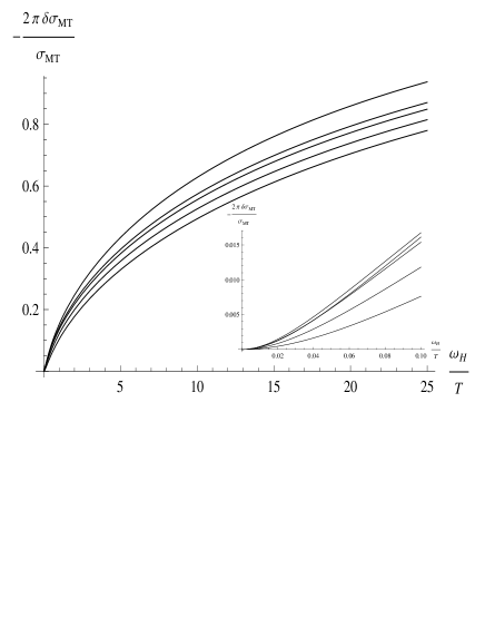
Figure 1: Normalized Maki-Thompson magnetoconductivity for 3$d$ case calculated at $T=1.8,3.5,4.4,6.0,8.0\,$K (top to bottom) with the corresponding dephasing times $\tau_{\phi}=(2.24,1.42,1.05,0.58,0.28)\times 10^{-10}$s. The material parameters are $D=6.37\times 10^{-4}$m²/s and $T_{c}=123$mK that correspond to Ref. Exp-3D-3, .

It is worth emphasizing that Eq. (9), taken at $\eta\to 0$, can be recovered from Eq. (Magnetoconductivity of low-dimensional disordered conductors at the onset of the superconducting transition) in the limit when $\omega_{H}\lesssim\tau_{\phi}^{-1}$, with the help of the approximate form of $Y_{3}(x)$ function [Eq. (3)], as it should be of course. The saturation region is not captured by Eq. (Magnetoconductivity of low-dimensional disordered conductors at the onset of the superconducting transition), but recovered correctly [Eq. (11)] within generalized formulation of MT magnetoconductivity. To facilitate the comparison between the theory [Eq. (7)] and experiments Exp-3D-1 ; Exp-3D-2 ; Exp-3D-3 ; Exp-3D-4 we plot on the Fig. 1 the MT magnetoconductivity at different temperatures for the material parameters taken from Ref. Exp-3D-3, . The inset plot in Fig. 1 emphasizes quadratic magnetic-field dependence of $\delta\sigma^{\mathrm{MT}}_{3}(H)$ at the lowest fields [see Eq. (9)].

For the two-dimensional case magnetoconductivity is determined by the following expression Santos-Abrahams ; Brenig-2 ; Reizer

$$\delta\sigma^{\mathrm{MT}}_{2}(H)=\frac{e^{2}}{\pi}\mathcal{B}(T)\left[Y_{2}(\omega_{H}\tau_{\mathrm{GL}})-Y_{2}(\omega_{H}\tau_{\phi})\right]\,,$$ (13)

where $Y_{2}(x)$ is defined by Eq. (2). For the same range of magnetic fields as in Eqs. (9)–(11) one finds from Eq. (13)

$$\hskip-25.6073pt\delta\sigma^{\mathrm{MT}}_{2}(H)=-\frac{e^{2}}{24\pi}\left[1+\frac{\tau_{\mathrm{GL}}}{\tau_{\phi}}\right](T\tau_{\mathrm{GL}})(\omega_{H}\tau_{\phi})^{2}\,,\,\,\omega_{H}\lesssim\tau_{\phi}^{-1}\!,$$ (14)

$$\hskip-25.6073pt\delta\sigma^{\mathrm{MT}}_{2}(H)=-\frac{e^{2}}{\pi}\frac{T\tau_{\mathrm{GL}}}{1-\frac{\tau_{\mathrm{GL}}}{\tau_{\phi}}}\ln\frac{\omega_{H}\tau_{\phi}}{4e^{\gamma_{E}}}\,,\,\,\tau_{\phi}^{-1}\lesssim\omega_{H}\lesssim\tau_{\mathrm{GL}}^{-1},$$ (15)

$$\hskip-25.6073pt\delta\sigma^{\mathrm{MT}}_{2}(H)=-\sigma^{\mathrm{MT}}_{2}(0)+\frac{\pi e^{2}}{2}\frac{T}{\omega_{H}}\,,\,\,\omega_{H}\gtrsim\tau_{\mathrm{GL}}^{-1},$$ (16)

where $\gamma_{E}=0.57..$ is the Euler constant. Similarly to the three-dimensional case MT magnetoconductivity saturates trough the series of crossovers $\delta\sigma^{\mathrm{MT}}_{2}(H)\propto H^{2}\to\ln H\to\mathrm{const}$, to its field independent value determined by Thompson

$$\sigma^{\mathrm{MT}}_{2}(0)=\frac{e^{2}}{\pi}\frac{T\tau_{\mathrm{GL}}}{1-\tau_{\mathrm{GL}}/\tau_{\phi}}\ln\frac{\tau_{\phi}}{\tau_{\mathrm{GL}}}\,.$$ (17)

By comparing Eq. (9) to Eq. (14) one concludes that quadratic field dependence, $\delta\sigma^{\mathrm{MT}}_{d}(H)\propto H^{2}$, at the lowest fields, $\omega_{H}\lesssim\tau_{\phi}^{-1}$, is apparently universal, in agreement with Eq. (Magnetoconductivity of low-dimensional disordered conductors at the onset of the superconducting transition), while magnetoconductivity saturation in the two-dimensional case is stronger then in the three dimensions.

At this point we discuss the role of Aslamazov-Larkin contribution to the magnetoconductivity and compare it to $\delta\sigma^{\mathrm{MT}}_{d}(H)$. In the two-dimensional case we find

$$\sigma^{\mathrm{AL}}_{2}(H)=\frac{2e^{2}}{\pi}(T\tau_{\mathrm{GL}})\mathcal{H}_{2}(\omega_{H}\tau_{\mathrm{GL}})\,,$$ (19)

$$\mathcal{H}_{2}(x)=\frac{1}{x}\left[1-\frac{2}{x}\left[\psi\left(1+\frac{1}{x}\right)-\psi\left(\frac{1}{2}+\frac{1}{x}\right)\right]\right]\,.$$

With the help of the asymptotic form of $\mathcal{H}_{2}$ function at zero field, $H\to 0$, where $\mathcal{H}_{2}(x\to 0)\to 1/4$, one recovers from Eq. (19) famous result Aslamazov-Larkin

$$\sigma^{\mathrm{AL}}_{2}(0)=\frac{e^{2}}{16}\frac{1}{\ln(T/T_{c})}\,.$$ (20)

Subtracting now $\sigma^{\mathrm{AL}}_{2}(0)$ from Eq. (19) for the two limiting cases of low, $\mathcal{H}_{2}(x)\approx\frac{1}{4}(1-\frac{x^{2}}{8})$, when $x\ll 1$, and high, $\mathcal{H}_{2}(x)\approx 1/x$, when $x\gg 1$, magnetic fields one finds:

$$\delta\sigma^{\mathrm{AL}}_{2}(H)=-\frac{e^{2}}{16\pi}(T\tau_{\mathrm{GL}})(\omega_{H}\tau_{\mathrm{GL}})^{2}\,,\,\,\omega_{H}\lesssim\tau_{\mathrm{GL}}^{-1}\,,$$ (21)

$$\delta\sigma^{\mathrm{AL}}_{2}(H)=-\sigma^{\mathrm{AL}}_{2}(0)+\frac{2e^{2}}{\pi}\frac{T}{\omega_{H}}\,,\,\,\omega_{H}\gtrsim\tau_{\mathrm{GL}}^{-1}\,,$$ (22)

which agrees also with the earlier results. Hikami-Larkin ; Abrahams ; Redi Similarly to Eqs. (9) and (14) the low-field Aslamazov-Larkin magnetoconductivity is universal and scales quadratically with $\omega_{H}$. It also saturates to the field independent value [Eq. (20)] at $\omega_{H}\gtrsim\tau_{\mathrm{GL}}^{-1}$, having the same $\sim 1/H$ correction as in Eq. (16). However, if one compares the magnitude of the MT and AL contributions, for example at $\omega_{H}\sim\tau_{\mathrm{GL}}^{-1}$, then it is easy to see from Eqs. (15) and (21) that $\delta\sigma^{\mathrm{MT}}_{2}(H)$ dominates against $\delta\sigma^{\mathrm{AL}}_{2}(H)$ by the logarithmic factor $\ln(\tau_{\phi}/\tau_{\mathrm{GL}})$ and this tendency persists for the smaller fields. Although $\ln(\tau_{\phi}/\tau_{\mathrm{GL}})$ depends on temperature, it actually stays practically constant, $\ln(\tau_{\phi}/\tau_{\mathrm{GL}})\sim 5$, at the experimentally addressed range of temperatures, 1K$\lesssim T\lesssim$10K in most of the measurements, see for example Refs. Exp-3D-3, and Exp-3D-4, . In the three-dimensional case expression similar to Eq. (19) can be derived, Hikami-Larkin which brings however the same conclusion about the relative importance of $\delta\sigma^{\mathrm{AL}}_{3}(H)$ when compared to $\delta\sigma^{\mathrm{MT}}_{3}(H)$ [Eq. (7)]. It should be emphasized that situation may be different if $\tau_{\mathrm{GL}}>\tau_{\phi}$, which may happen in the layered superconductors. For this case $\delta\sigma^{\mathrm{AL}}_{d}(H)$ dominates the magnetotransport in the vicinity of the critical temperature. Hikami-Larkin ; Dorin

In the remaining part of the paper we outline the essential steps needed to derive Eqs. (7)–(19). Within the linear response Keldysh technique, which is proven to be very effective tool in application to the transport problems of fluctuating superconductors, Reizer ; LK Maki-Thompson conductivity correction is determined by the following expression

$$\sigma^{\mathrm{MT}}_{d}=\frac{e^{2}D}{2\pi}\sum_{q}\iint^{+\infty}_{-\infty}\frac{\mathrm{d}\epsilon\mathrm{d}\omega}{\cosh^{2}\frac{\epsilon}{2T}}\,\mathrm{Im}\big{[}L^{R}(q,\omega)\big{]}$$

$$\big{|}C^{R}(q,2\epsilon+\omega)\big{|}^{2}\left[\coth\frac{\omega}{2T}-\tanh\frac{\epsilon+\omega}{2T}\right]\,.$$ (23)

Here interaction propagator is given by $L^{R}(q,\omega)=\left[\ln\frac{T}{T_{c}}+\psi\left(\frac{Dq^{2}-i\omega}{4\pi T}+\frac{1}{2}\right)-\psi\left(\frac{1}{2}\right)\right]^{-1}$, while $C^{R}(q,\omega)=\left[Dq^{2}-i\omega+\tau_{\phi}^{-1}\right]^{-1}$ stands for the Cooperon. In the three-dimensional case with magnetic field pointed along the $z$ axes one has $Dq^{2}\to Dq^{2}_{z}+\omega_{H}(n+1/2)$ and momentum summation in Eq. (Magnetoconductivity of low-dimensional disordered conductors at the onset of the superconducting transition) is performed as $\sum_{q}\to\frac{\omega_{H}}{4\pi D}\int^{+\infty}_{-\infty}\frac{\mathrm{d}q_{z}}{2\pi}\sum^{\infty}_{n=0}$, where the prefactor conventionally accounts for the degeneracy in the position of Landau orbit. Passing to the dimensionless units $x=Dq^{2}_{z}/T$, $y=\omega/T$, $z=\epsilon/T$, and $w_{n}=\frac{\omega_{H}}{T}(n+1/2)$ Eq. (Magnetoconductivity of low-dimensional disordered conductors at the onset of the superconducting transition) can be reduced to

$$\sigma^{\mathrm{MT}}_{3}(H)=\frac{e^{2}}{2\pi^{4}\ell_{T}}\frac{\omega_{H}}{T}\sum^{\infty}_{n=0}\int^{+\infty}_{0}\frac{\mathrm{d}x}{\sqrt{x}}\iint^{+\infty}_{-\infty}\!\!\frac{\mathrm{d}z\mathrm{d}y}{\cosh^{2}\frac{z}{2}}$$

$$\frac{y\big{[}\coth\frac{y}{2}-\tanh\frac{z+y}{2}\big{]}}{\big{[}\big{(}x+w_{n}+\frac{1}{T\tau_{\mathrm{GL}}}\big{)}^{2}+y^{2}\big{]}\big{[}\big{(}x+w_{n}+\frac{1}{T\tau_{\phi}}\big{)}^{2}+(2z+y)^{2}\big{]}}\,,\qquad$$ (24)

where we expanded interaction propagator $L^{R}(q,\omega)$ at small frequencies and momenta, assuming $\mathrm{max}\{Dq^{2},\omega\}\ll 4\pi T$. One sees from Eq. (Magnetoconductivity of low-dimensional disordered conductors at the onset of the superconducting transition) that the relevant range for $z$ integration is set by $z\sim 1$, whereas the width of the Cooperon is determined by $\mathrm{max}\{x,w_{n},(T\tau_{\phi})^{-1}\}\ll 1$. At the end, this condition limits applicability of Eq. (7) to magnetic fields not exceeding $\omega_{H}\lesssim 4\pi T$, which is still sufficient to explain the magnetoconductivity saturation happening at $\omega_{H}\sim\tau_{\mathrm{GL}}^{-1}\ll T$. Under this assumption one is allowed to approximate $\big{|}C^{R}(x+w_{n},2z+y)\big{|}^{2}\approx\frac{\pi}{x+w_{n}+\frac{1}{T\tau_{\phi}}}\delta(2z+y)$ in Eq. (Magnetoconductivity of low-dimensional disordered conductors at the onset of the superconducting transition). Integration over $z$ becomes immediate and gives

$$\sigma^{\mathrm{MT}}_{3}(H)=\frac{e^{2}}{4\pi^{3}\ell_{T}}\frac{\omega_{H}}{T}\sum^{\infty}_{n=0}\int^{+\infty}_{0}\frac{\mathrm{d}x}{\sqrt{x}\big{[}x+w_{n}+\frac{1}{T\tau_{\phi}}\big{]}}$$

$$\int^{+\infty}_{-\infty}\frac{\mathrm{d}y}{\cosh^{2}\frac{y}{4}}\frac{y\big{[}\coth\frac{y}{2}-\tanh\frac{y}{4}\big{]}}{\big{[}\big{(}x+w_{n}+\frac{1}{T\tau_{\mathrm{GL}}}\big{)}^{2}+y^{2}\big{]}}\,.$$ (25)

The $y$ integration can be completed with the same line of reasoning as in the $z$ case, assuming that $\mathrm{max}\{x,w_{n},(T\tau_{\mathrm{GL}})^{-1}\}\ll 1$, which is consistent with the previous step, and gives a factor $2\pi/(x+w_{n}+1/T\tau_{\mathrm{GL}})$. After that step summation over $n$ is straightforward with the help of the digamma function. Rescaling also $x\to(\omega_{H}/T)t$ one obtains from Eq. (Magnetoconductivity of low-dimensional disordered conductors at the onset of the superconducting transition)

$$\sigma^{\mathrm{MT}}_{3}(H)=\frac{e^{2}}{2\pi^{2}\ell_{H}}\mathcal{B}(T)\int^{+\infty}_{0}\frac{\mathrm{d}t}{\sqrt{t}}\left[\psi\left(\frac{1}{2}+t+\frac{1}{\omega_{H}\tau_{\mathrm{GL}}}\right)\right.$$

$$\left.-\psi\left(\frac{1}{2}+t+\frac{1}{\omega_{H}\tau_{\phi}}\right)\right]\,.$$ (26)

To recover Eq. (12) from Eq. (Magnetoconductivity of low-dimensional disordered conductors at the onset of the superconducting transition) at zero magnetic field one uses following asymptote $\psi\big{(}\frac{1}{2}+t+\frac{1}{x}\big{)}\stackrel{{\scriptstyle x\to 0}}{{\longrightarrow}}\ln\big{(}t+\frac{1}{x}\big{)}$ and an integral identity $\int^{\infty}_{0}\frac{\mathrm{d}t}{\sqrt{t}}\ln\big{(}\frac{t+a}{t+b}\big{)}=2\pi\big{[}\sqrt{a}-\sqrt{b}\big{]}$. As the final step one subtracts Eq. (12) from Eq. (Magnetoconductivity of low-dimensional disordered conductors at the onset of the superconducting transition) and arrives at our major result given by Eq. (7). Corresponding calculations for the two-dimensional case [Eq. (13)] as well as derivation of Aslamazov-Larkin contribution [Eq. (19)] are completely analogous.

In conclusion we have suggested the complete theoretical description of the magnetotransport in fluctuating regime of superconductors of different dimensionality. Interaction corrections in the Cooper channel play the dominant role and are governed by the Maki-Thompson contribution. Sufficiently strong magnetic field suppresses fluctuation effects completely and magnetoconductivity is determined then by the weak-localization effect. At the immediate vicinity of the critical temperature Aslamazov-Larkin correction may become more important and one may observe MT$\to$AL or dimensional crossovers. These theoretical results are in good agreement with the experimental observations. Exp-3D-1 ; Exp-3D-2 ; Exp-3D-3 ; Exp-3D-4

This research was supported in part by the National Science Foundation under Grants No. PHY05-51164, No. DMR-0405212, and No. DMR-0804266.

References

- (1) S. Hikami. A. I. Larkin, and Y. Nagaoka, Prog. Theor. Phys. 63, 707 (1980).
- (2) B. L. Altshuler and A. G. Aronov, in Electron-Electron Interaction in Disordered Systems, edited by A. J. Efros and M. Pollak (Elsevier, Amsterdam, 1985), pp. 1-153.
- (3) A. I. Larkin and A. Varlamov, Theory of fluctuations in superconductors (Clarendon Press, Oxford, 2005).
- (4) L. G. Aslamazov and A. I. Larkin, Fiz. Tverd. Tela 10, 1104 (1968) [Soviet Phys. Solid. State 10, 875 (1968)].
- (5) K. Maki, Prog. Theor. Phys. 39, 897 (1968).
- (6) R. S. Thompson, Phys. Rev. B 1, 327 (1970).
- (7) A. I. Larkin, Pis’ma Zh. Eksp. Teor. Fiz. 31, 239 (1980) [JETP Lett. 31, 219 (1980)].
- (8) B. L. Altshuler, A. G. Aronov, A. I. Larkin, and D. E. Khmelnitskii, Zh. Eksp. Teor. Fiz. 81, 768 (1981) [Sov. Phys. JETP 54, 411 (1981)].
- (9) B. L. Altshuler, D. Khmel’nitzkii, A. I. Larkin, and P. A. Lee, Phys. Rev. B 22, 5142 (1980).
- (10) A. Kawabata, Solid State Commun.34, 431 (1980).
- (11) Y. Bruynseraede, M. Gijs, C. Van Haesendonck, and G. Deutscher, Phys. Rev. Lett. 50, 277 (1983).
- (12) R. Rosenbaum, Phys. Rev. B 32, 2190 (1985).
- (13) J. M. Gordon and A. M. Goldman, Phys. Rev. B 34, 1500 (1986).
- (14) B. Shinozaki and L. Rinderer, J. Low Temp. Phys. 73, 267 (1988).
- (15) C. Y. Wu and J. J. Lin, Phys. Rev. B 50, 385 (1994).
- (16) H. Fujiki, M. Yamada, B. Shinozaki, T. Kawaguti, F. Ichikawa, T. Fukami, and T. Aomine, Physica C 311, 58 (1999).
- (17) K. Meiners-Hagen and W. Gey, Phys. Rev. B 63, 052507 (2001).
- (18) R. Rosenbaum, S. Y. Hsu, J. Y. Chen, Y. H. Lin, and J. J. Lin, J. Phys.: Condens. Matter 13, 10041 (2001).
- (19) J. J. Lin and J. P. Bird, J. Phys.: Condens. Matter 14, R501 (2002).
- (20) J. M. B. Lopes dos Santos and E. Abrahams, Phys. Rev. B 31, 172 (1985).
- (21) W. Brenig, J. Low Temp. Phys. 60, 297 (1985).
- (22) W. Brenig, M. A. Paalanen, A. F. Hebard, and P. Wölfle, Phys. Rev. B 33, 1691 (1986).
- (23) M. Yu. Reizer, Phys. Rev. B 45, 12949 (1992).
- (24) S. Hikami and A. I. Larkin, Mod. Phys. Lett. B 2, 693 (1988).
- (25) V. V. Dorin, R. A. Klemm, A. A. Varlamov, A. I. Buzdin, and D. V. Livanov, Phys. Rev. B 48, 12951 (1993).
- (26) E. Abrahams, R. E. Prange, and M. J. Stephen, Physica 55, 230 (1971).
- (27) M. H. Redi, Phys. Rev. B 16, 2027 (1977).
- (28) A. Levchenko and A. Kamenev, Phys. Rev. B 76, 094518 (2007).