Hard sphere fluids in annular wedges: density distributions and depletion potentials

Abstract

We analyze the density distribution and the adsorption of solvent hard spheres in an annular slit formed by two large solute spheres or a large solute and a wall at close distances by means of fundamental measure density functional theory, anisotropic integral equations and simulations. We find that the main features of the density distribution in the slit are described by an effective, two–dimensional system of disks in the vicinity of a central obstacle. This has an immediate consequence for the depletion force between the solutes (or the wall and the solute), since the latter receives a strong line–tension contribution due to the adsorption of the effective disks at the circumference of the central obstacle. For large solute–solvent size ratios, the resulting depletion force has a straightforward geometrical interpretation which gives a precise “colloidal” limit for the depletion interaction. For intermediate size ratios 5 …10 and high solvent packing fractions larger than 0.4, the explicit density functional results show a deep attractive well for the depletion potential at solute contact, possibly indicating demixing in a binary mixture at low solute and high solvent packing fraction.

I Introduction

The equilibrium statistical theory of inhomogeneous fluids whose foundations were laid out in the 1960’s Mor60 ; Ste64 is a well–studied subject which has been developed since by a fruitful interplay between simulations and theory. For the simplest molecular model, the hard–body fluid mixture, this has led to the development of powerful, geometry–based density functionals Ros89 ; Rot02 ; Yu02 ; Han06 ; Mal06 ; Han09 which accurately describe adsorption phenomena, phase transitions (such as freezing for pure hard spheres or demixing for entropic colloid–polymer mixtures) and molecular layering near obstacles. Such a class of density functionals has not been found yet for fluids with attractions, however, significant progess has been achieved in the description of bulk correlation functions and phase diagrams through the method of integral equations Pin02 ; Par08 ; Aya09 .

Strong inhomogeneities occur if fluids are confined on molecular scales, a topic which enjoys continuous interest Tru08 ; Jun08 . For example, the packing of molecules between parallel walls leads to oscillating forces between them which can be measured experimentally and determined theoretically Isr . With the development of preparational techniques for colloids and their mixtures, the “molecular” length scale has been lifted to the range of several nm up to $\mu$m which even allows the direct observation of modulated density profiles through microscopy besides the measurement of resulting forces on the walls. Furthermore, in the colloidal domain the possibility to tailor the interparticle interactions to a certain degree allows the close realization of some of the favourite models for simple fluids fancied by theorists, such as e.g. hard spheres Dul06 . This has opened the route to quantitative comparisons between experiment, theory and simulations.

In an asymmetric colloidal mixture with small “solvent” particles and at least one species of larger solute particles, the phenomenon of solvent–mediated, effective interactions between the solute particles may give rise to various phase separation phenomena Lik01 . From a theoretical point of view, these effective interactions are interesting since they facilitate the description of mixtures in terms of an equivalent theory for one species interacting by an effective potential McMillan45 ; Dij99 . If the solvent particles possess hard (or at least steeply repulsive) cores, they are excluded from the region between two solute particles if the latter are separated by less than one solvent diameter. This gives rise to strong depletion forces whose understanding is crucial for the concept of an effective theory containing only solute degrees of freedom. Since the magnitude of the depletion force is directly linked to the solvent density distribution around the solutes, the quantitative investigation of the solvent confined between solute particles appears to be important. The confinement becomes rather extreme for large asymmetry between solute and solvent (see below).

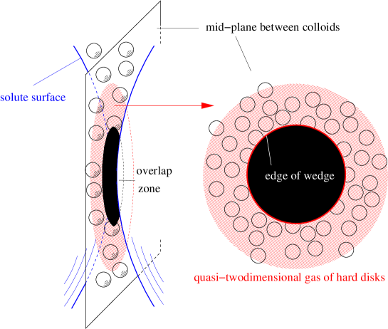
Figure 1: (color online) The annular wedge which is formed between two large solute particles for separations $h\leq\sigma$. Black areas denote domains which are forbidden for the centers of the solvent spheres.

In the following we want to concentrate on the idealized system of additive hard spheres and in particular on the effective interaction between two solute particles in solvent, i.e. the case of infinite dilution of solute particles in the colloidal mixture. The case of the interaction of one solute particle with a wall is a special case in that the radius of the other solute particle goes to infinity. For the case of hard spheres (solvent diameter $\sigma=2R_{s}$, solute radius $R_{b}$ such that the size ratio is $\alpha=R_{b}/R_{s}$ and $R=R_{b}+R_{s}$ is the radius of the exclusion sphere for solvent centres around a solute sphere) it has been found that the theoretical description using “bulk” methods becomes increasingly inaccurate for size ratios $\alpha\gtrsim 5$ and solvent densities $\rho_{s}^{*}=\rho_{s}\sigma^{3}\gtrsim 0.6$, when compared to simulations. Here, the terminus “bulk” methods refers to methods which determine the bulk pair correlation function between the colloids, $g_{bb}(r)$, from which the depletion potential is obtained as $\beta W=-\ln g_{bb}$. Bulk integral equation (IE) methods Att90 and the “insertion” trick in density functional theory (DFT) Rot00 ; Amo01 ; Aya05 ; Amo07 fall into this category. For larger size ratio, one would expect that the well–known Derjaguin approximation Der34 ; Hen02 ; Oet04 becomes accurate very quickly. Interestingly, however, both the mentioned bulk methods and simulations deviate significantly from the Derjaguin approximation (besides disagreeing with each other) for size ratios 10 and solvent densities $\rho_{s}^{*}=0.6\dots 0.7$ Bib96 ; Dic97 ; Oet04 when the surface–to–surface separation $h$ between the solute particles is close to $\sigma$ ($h\lesssim\sigma$, i.e. at the onset of the depletion region where the solvent particles are “squeezed out” between the solute particles). One notices that for $h\leq\sigma$ the solute particles form an annular wedge with a sharp edge which restricts the solvent particles to quasi–2d motion (see Fig. 1). Taking this observation into account, the phenomenological analysis of Ref. Oet04 predicted that the solvent adsorption at this edge leads to a line contribution to the depletion potential which is proportional to the circumference of the circular egde and thus to $R^{1/2}$. Such a term in the depletion potential causes a very slow approach to the Derjaguin limit for large solutes (the Derjaguin approximation describes the depletion potential essentially by volume and area terms of the overlap of the exclusion spheres pertaining to the solutes Hen02 ; Oet04 , see below). In this way, a generalized Derjaguin approximation serving as a new “colloidal” limit can be formulated which turns out to have a far more general meaning Oet09 than anticipated. Using the concept of morphological (morphometric) (morphometric) (morphometric) (morphometric) (morphometric) (morphometric) (morphometric) (morphometric) thermodynamics introduced in Ref. Koe04 , one finds that the insertion free energy of two solute particles (and thus the depletion potential between them) only depends on the volume, surface area, and the integrated mean and Gaussian curvatures of the solvent accessible surface around the two solutes. The coefficients of these four terms depend on the solvent density but not on the specific type of surface. In this manner, the phenomenological line tension of Ref. Oet04 is related to the general coefficient of mean curvature of the hard–sphere fluid Oet09 , and the Derjaguin approximation is equivalent to the morphometric analysis restricted to volume and surface area terms.

Since the depletion force in the hard–sphere system is directly linked to an integral over the solvent contact density on one solute (see Eqs. (II) and (2) below), one should be able to connect the morphometric approach to features of the solvent density profile in the annular wedge. This is a strong motivation for us to explicitly determine the wedge density profile. We will do so by means of density functional theory and anisotropic integral equations, and compare it to results of Monte–Carlo (MC) simulations for selected parameters. For the intermediate densities $\rho_{s}^{*}=0.6$ and $0.7$ and various size ratios between solute and solvent results for the depletion force from such explicit DFT calculations were already presented in Ref. Oet09 , and good agreement with the morphometric depletion force was obtained for size ratios between 5 and 40. Here, we will present a detailed analysis of the wedge density profiles and consider also higher densities. We will give a thorough comparison to recent results from MC simulations which have been obtained for the wall–solute interaction at a solvent density $\rho_{s}^{*}=0.764$ ($\eta_{s}=(\pi/6)\rho_{s}\sigma^{3}=0.4$) and size ratios between 10 and 100 Her06 ; Her07 ; Her08 .

The paper is structured as follows. In Sec. II we introduce the basic notions of density functional and integral equation theory and present a short description of the Monte Carlo simulations employed here. In Sec. III.1 we analyze in detail the density profiles and the corresponding depletion forces for the wall–sphere geometry for the particular solvent density $\rho_{s}^{*}=0.764$. This geometry permits explicit calculations up to solute–solvent size ratios 100 and a test of the “colloidal limit” of the morphometric depletion force. Sec. III.2 gives an analysis of the depletion force and potential in the sphere–sphere geometry (corresponding to the important case of the effective interaction in a dilute mixture) for intermediate size ratios 5 and 10 and higher solvent densities $\rho_{s}^{*}=$ 0.8 …0.9.

II Theory and methods

We consider two scenarios (see Fig. 2): (a) One hard solute sphere immersed in the hard sphere solvent of density $\rho_{s}$ confined to a slit, created by two hard walls at distance $L$. The surface–to–surface distance between one wall and the solute sphere is denoted by $h$, furthermore $L\gg h$ such that the correlations from one wall do not influence the solute interaction with the other wall. (b) Two hard solute spheres immersed in the bulk solvent spheres with surface–to–surface distance $h$. The solvent accessible surface is given by the dashed lines in Fig. 2, thereby one sees that for $h\leq\sigma$ the two solutes (or the solute and one wall) form an annular wedge in which the solvent adsorbs. The solvent density profile $\rho(\mathbf{r})\equiv\rho(r_{||},z)$ depends only on $z$, the coordinate on the symmetry axis and the distance $r_{||}$ to the symmetry axis. In the latter case (b), when the first colloid is centered at the origin and the second one at $z=2R_{b}+h$, the total force $f(h)$ on the first colloid is obtained by integrating the force $-\nabla u_{bs}(\mathbf{r})$ ($u_{bs}$ is the solute–solvent potential) between the solute and one solvent sphere over the density distribution $\rho(\mathbf{r})$:

$$\beta f(h) = -\int d^{3}r\;\rho(\mathbf{r})\;\mathbf{e}_{z}\cdot\nabla u_{bs}(\mathbf{r})$$

$$= 2\pi R^{2}\;\int_{-1}^{1}d(\cos\theta)\cos\theta\;\rho(\mathbf{r})\;,$$

$$\quad\left[|\mathbf{r}|=R\;,\quad\cos\theta=\hat{\mathbf{r}}\cdot\mathbf{e}_{z}\right]\;.$$

Thus the total depletion force reduces to an integral over essentially the contact density on the exclusion sphere around the colloid. This follows from $\exp(-\beta u_{bs})\beta\nabla u_{bs}=-\hat{\mathbf{r}}\delta(|\mathbf{r}|-R)$ and the observation that $\rho(\mathbf{r})\exp(\beta u_{bs})$ is continuous across the exclusion sphere surface. In case (a), the force on the colloid is the negative of the excess force $f_{w}$ on the wall and the excess force is determined by the total force on the wall minus the contribution from the bulk solvent pressure $p$. Through the wall theorem, the latter is given by $\beta p=\rho_{w}$ where $\rho_{w}$ is the contact density of the solvent at a single wall. By an argument similar to the above one and putting the exclusion surface of the wall at $z=0$, $f_{w}$ is determined as

$$\beta f_{w}(h) = -2\pi\int_{0}^{\infty}r_{||}\,dr_{||}\;(\rho(r_{||},z=0)-\rho_{w})\;.$$ (2)

Thus, $f_{w}$ is equivalent to the excess adsorption at the wall which makes it somewhat easier to determine in MC simulations than $f$ Her07 .

(a)
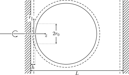
(b)

Figure 2: View of the geometric configurations used in this work. (a) Solute sphere of radius $R_{b}$ immersed in a solvent–filled slit of width $L$. Only the density profile in the annular wedge between the left wall and the solute is of interest since it determines the depletion force between solute and one wall. Note that one can also determine the slit density profile and the corresponding depletion force for $2R_{b}>L$ (i.e. when the solute does not fit into the slit) as long as $L$ is large enough that the correlations from the right wall do not reach into the annular wedge. (b) Two solute spheres of radius $R_{b}$ at distance $h$ immersed in bulk solvent. For both setups, the solvent sphere diameter is given by $\sigma$, and the radius of the exclusion sphere around a solute particle is given by $R=R_{b}+\sigma/2$.

II.1 Density functional theory

The equilibrium solvent density profile $\rho(\mathbf{r})\equiv\rho_{\rm eq}(\mathbf{r})$ can be determined directly from the basic equations of density functional theory. The grand potential functional is given by

$$\Omega[\rho] = {\cal F}^{\rm id}[\rho]+{\cal F}^{\rm ex}[\rho]-\int d\mathbf{r}(\mu-V^{\rm ext}(\mathbf{r}))\;,$$ (3)

where ${\cal F}^{\rm id}$ and ${\cal F}^{\rm ex}$ denote the ideal and excess free energy functionals of the solvent. The solvent chemical potential is denoted by $\mu$ and the solute(s) and/or the walls define the external potential $V^{\rm ext}$. The ideal part of the free energy is given by

$$\beta{\cal F}^{\rm id} = \int d\mathbf{r}\,\rho(\mathbf{r})\left(\ln(\rho(\mathbf{r})\Lambda^{3})-1\right)\;,$$ (4)

with $\Lambda$ denoting the de–Broglie wavelength. The equilibrium density profile $\rho_{\rm eq}(\mathbf{r})$ for the solvent at chemical potential $\mu=\beta^{-1}\ln(\rho_{s}\,\Lambda^{3})+\mu^{\rm ex}$ (corresponding to the bulk density $\rho_{s}$) is found by minimizing the grand potential in Eq. (3):

$$\ln\frac{\rho_{\rm eq}(\mathbf{r})}{\rho_{s}}+\beta V^{\rm ext}(\mathbf{r})=-\beta\frac{\delta{\cal F}^{\rm ex}[\rho_{\rm eq}]}{\delta\rho(\mathbf{r})}+\beta\mu^{\rm ex}\;.$$ (5)

For an explicit solution, it is necessary to specify the excess part of the free energy. Here we employ two functionals of fundamental measure type (FMT). These are the original Rosenfeld functional (FMT–RF) Ros89 and the White Bear functional (FMT–WB, with Mark I from Refs. Rot02 ; Yu02 and Mark II from Ref. Han06 ), for another closely related variant see Ref. Mal06 . It has been demonstrated that FMT gives very precise density profiles also for high densities of the hard sphere fluid in various circumstances. Furthermore, the White Bear II functional possesses a high degree of self–consistency with regard to scaled–particle considerations Han06 . However, we do not consider the tensor–weight modifications of these functionals which are necessary to obtain a correct description of the liquid–solid transition Tar00 and are of higher consistency in confining situations which reduce the dimensionality of the system (“dimensional crossover”, see Ref. Tar97 ; Ros97 ). This might be an issue in some circumstances (see below).

Th explicit forms of the excess free energy are given in App. B. Numerically, due to the non–local nature of ${\cal F}^{\rm ex}$, Eq. (5) corresponds to an integral equation for the density profile depending on the two variables $r_{||}$ and $z$. The sharpness of the annular wedge in the solute–solute and the solute–wall problems for high size ratios necessitates rather fine gridding (which makes the calculation of ${\cal F}^{\rm ex}$ and $\delta{\cal F}^{\rm ex}/\delta\rho$ very time–consuming) and introduces an unusual slowing–down of standard iteration procedures of Picard type. To overcome these difficulties, we made use of fast Hankel transform techniques and more efficient iteration procedures. These are described in detail in App. B as well.

We remark that there have been earlier attempts to obtain explicit density distributions using DFT around two fixed solutes and thereby to extract depletion forces Arc05 ; Ego04 ; Gou01 . In Ref. Ego04 this was done using the simple Tarazona I functional for hard spheres Tar84 , and considerations were limited to a small solvent packing fraction of 0.1 and solute–solvent size ratios of 5. In Ref. Gou01 , a minimization of FMT–RF was carried out using a real–space technique for solvent densities up to $\rho_{s}^{*}=0.6$ and size ratios 5. In that respect, the present technique is superior in that it allows us to present solutions for solvent densities up to $\rho_{s}^{*}=0.9$ and size ratios up to 100.

II.2 Integral equations

The central objects within the theory of integral equations are the correlation functions on the one and two–particle level in the solvent. We are interested in the two–particle correlation functions in the presence of an external background potential (one fixed object, solute or wall), from which the explicit solvent density profiles around the two fixed objects (solute–solute or solute–wall) follow (see below). This is usually referred to as the method of inhomogeneous or anisotropic integral equations, first employed for Lennard–Jones fluids on solid substrates Hillebrand84 ; Bruno87 and for hard–spheres (HS) fluids in contact with a single hard wall in Ref. Plischke86 . Liquids confined between two parallel walls (a planar slit) have been extensively studied by Kjellander and Sarman Kjellander88 ; Kjellander90 ; Kjellander91 .

For an arbitrary background potential $V(\mathbf{r})$ which corresponds to an equilibrium background density profile for the solvent $\rho_{V}(\mathbf{r})$, the pair correlation function $g_{ij}(\mathbf{r},\mathbf{r}_{0})=h_{ij}(\mathbf{r},\mathbf{r}_{0})+1$ describes the normalized probability to find a particle of species $i$ at position $\mathbf{r}$ if another particle of species $j$ is fixed at position $\mathbf{r}_{0}$. For our system, the species index is either $s$ (solvent particle) or $b$ (big solute particle). In the solute–solute case, $V$ is given by the potential of one solute particle, whereas in the solute–wall case it is the potential of the wall. Then the equilibrium density profile discussed in the previous subsection is related to the pair correlation function through $\rho(\mathbf{r})=\rho_{V}(\mathbf{r})\,g_{sb}(\mathbf{r},\mathbf{r}_{0})$ ($\mathbf{r}_{0}$ specifies the position of the (other) solute particle). The depletion force follows then through Eqs. (II) and (2).

The corresponding direct correlation functions of second order $c_{ij}(\mathbf{r},\mathbf{r}_{0})$ are related to $h_{ij}$ through the inhomogeneous Ornstein–Zernike (OZ) equations

$$h_{ij}(\mathbf{r},\mathbf{r}_{0})-c_{ij}(\mathbf{r},\mathbf{r}_{0})=\sum_{k=b,s}\int d\mathbf{r}^{\prime}\rho_{V,k}(\mathbf{r}^{\prime})h_{ik}(\mathbf{r},\mathbf{r}^{\prime})c_{kj}(\mathbf{r}^{\prime},\mathbf{r}_{0})$$ (6)

In the dilute limit for the solute particles which we consider here, the background density $\rho_{V,b}$ for the solutes is zero, therefore the OZ equations reduce to

$$h_{ss}(\mathbf{r},\mathbf{r}_{0})-c_{ss}(\mathbf{r},\mathbf{r}_{0}) = \int d\mathbf{r}^{\prime}\rho_{V}(\mathbf{r}^{\prime})h_{ss}(\mathbf{r},\mathbf{r}^{\prime})c_{ss}(\mathbf{r}^{\prime},\mathbf{r}_{0})\;,$$ (7)

$$h_{bs}(\mathbf{r},\mathbf{r}_{0})-c_{bs}(\mathbf{r},\mathbf{r}_{0}) = \int d\mathbf{r}^{\prime}\rho_{V}(\mathbf{r}^{\prime})h_{bs}(\mathbf{r},\mathbf{r}^{\prime})c_{ss}(\mathbf{r}^{\prime},\mathbf{r}_{0})\;.$$ (8)

The background density profile is linked to $c_{ss}$ through the Lovett–Mou–Buff–Wertheim equation LMBW :

$$\nabla\rho_{V}(\mathbf{r})=-\beta\rho_{V}(\mathbf{r})\nabla V(\mathbf{r})+\rho_{V}(r)\int d\mathbf{r}^{\prime}c_{ss}(\mathbf{r},\mathbf{r}^{\prime})\nabla\rho_{V}(\mathbf{r}^{\prime})\;.$$ (9)

A third set of equations is necessary to close the system of equations. The diagrammatic analysis of Ref. Mor60 provides the general form of this closure which reads:

$$\ln g_{ij}(\mathbf{r},\mathbf{r}_{0})+\beta u_{ij}(\mathbf{r}-\mathbf{r}_{0}) = h_{ij}(\mathbf{r},\mathbf{r}_{0})-c_{ij}(\mathbf{r},\mathbf{r}_{0})-b_{ij}(\mathbf{r},\mathbf{r}_{0})\;,$$ (10)

where $u_{ij}$ are the pair potentials in the solute–solvent mixture and $b_{ij}$ denote the bridge functions specified by a certain class of diagrams which, however, can not be resummed in a closed form. For practical applications, these bridge functions need to be specified in terms of $h_{ij}$ and $c_{ij}$ to arrive at a closed system of equations. Among the variety of empirical forms devised for this connection we mention those which, in our opinion, rely on somewhat more general arguments. These are the venerable hypernetted chain (HNC), Percus–Yevick (PY) closure and the mean spherical approximation (MSA) which can be derived by systematic diagrammatic arguments HMD06 , and the reference HNC closure which introduces a suitable reference system for obtaining $b_{ij}$ with subsequent free energy minimization Lad83 . (For bulk properties of liquids, the self–consistent Ornstein–Zernike approximation (SCOZA) Pin02 and the hierarchical reference theory (HRT) Par08 are very successful. They rely on a closure of MSA type but it appears to be difficult in generalizing them to inhomogeneous situations such as considered here.) In calculations, we considered the closures

$$b_{ij} = \gamma_{ij}-\ln(1+\gamma_{ij})\qquad\mbox{(PY)}\;,$$ (11)

$$b_{ij} = \gamma_{ij}-\ln\left[1+\frac{\exp\{[1-\exp(-\xi_{ij}r)]\gamma_{ij}\}-1}{1-\exp(-\xi_{ij}r)}\right]\qquad\mbox{(RY)}\;,$$ (12)

$$b_{ij} = \frac{1}{2}\frac{\gamma_{ij}^{2}}{1+\alpha_{ij}\gamma_{ij}}\qquad\mbox{(MV)}\;.$$ (13)

where $\gamma_{ij}=h_{ij}-c_{ij}$. The Percus–Yevick (PY) approximation Eq. (11) is exactly solvable in the bulk case even for the muticomponent HS fluid Lebowitz . However, beyond providing good qualitative behavior PY does not produce precise quantitative results in general, since it fails at contact, where the value of pair distribution function is too small. For bulk systems, PY generates a noticeable thermodynamic inconsistency, i.e. a discrepancy between different routes to the equation of state. To overcome these deficiencies a refined approximation to the closure, which interpolates between HNC ($b_{ij}=0$) and PY closures was suggested by Rogers and Young (RY) RY , see Eq. (12) where the $\xi_{ij}$ are adjustable parameters, which can be found from the thermodynamic consistency requirement RY . An even more suitable for the asymmetric HS mixtures variant of the modified Verlet (MV) closure was suggested in Ref. Henderson96 , see Eq. (13). Here the parameters $\alpha_{ij}$ are chosen to satisfy the exact relation between $b_{ij}(0)$ and the third virial coefficient at low densities. For the choice of the auxiliary parameters $\xi_{ij}$ and $\alpha_{ij}$ in the present work, see App. C

We have solved the set of equations (7)–(13) for the solute–wall case where we could employ similar numerical methods as in the numerical treatment of density functional theory. (This is not possible for the solute-solute case, for an efficient method applicable in this case, see Ref. Att89 .) In the solute–wall case, the background density profile $\rho_{V}(\mathbf{r})\equiv\rho_{V}(z)$ depends only on the distance $z$ from the wall. The two–particle correlation functions depend on the $z$–coordinates of the two particles individually and the difference in the radial coordinates: $g_{ij}(\mathbf{r},\mathbf{r}_{0})\equiv g_{ij}(z,z_{0},r_{||}-r_{||,0})$. Thus, the Ornstein–Zernike equations (7) and (8) become matrix equations for the correlation functions in the $z$–coordinates, and are diagonal for the Hankel transforms of the correlation functions in the $r_{||}$–coordinates. For more details on the numerical procedure, see App. C.

II.3 Simulation Details

The Monte Carlo simulations for the wall–solute system were performed at fixed particle number and volume of the simulation box. The upper boundary of the box was given by a large hard sphere, the lower boundary by a planar hard wall (see hatched regions in Fig. 3). All remaining boundaries were treated as periodic. We sampled the configuration space of the small spheres by standard single particle translational moves. In order to impose the asymptotic solvent bulk density $\rho_{s}^{*}=0.764$ ($\eta_{s}=0.4$), the concentration of small spheres in the box was set such that the density at contact with the hard wall far away from the wedge (i. e. in the region marked by grey squares in Fig. 3, averaged over a depth 0.02 $\sigma$) settled to $\bar{\rho}_{\rm Wall}=4.88$ within 1% error. This value $\bar{\rho}_{\rm Wall}=4.88$ was obtained from the density profile of hard spheres at a hard wall at the bulk packing fraction 0.4, calculated with FMT–WBII which is very accurate. System sizes ranged from 1800 particles for $R_{b}=10\;\sigma$ to 8000 particles for $R_{b}=25\;\sigma$. In order to access the configurations inside the narrow part of the wedge with sufficient accuracy, large numbers of Monte Carlo sweeps were required. We equilibrated the systems for $5\times 10^{5}$ MC sweeps (i. e. attempted moves per particle) each. For data acquisition, we performed between $10^{7}$ and $10^{8}$ sweeps (depending on the parameters $h$ and $R_{b}$) and averaged over $10^{6}$ to $10^{7}$ samples. Note that from the simulations we obtained only the wedge density profiles (see Figs. 5–7 below) but did not attempt to obtain the depletion force from Eq. (2) where one needs an excess adsorption integral at the wall. This would require considerably more sweeps Her07 ; Her08 , see also Fig. 8 below for the statistical errors of the simulated depletion force according to Ref. Her07 .

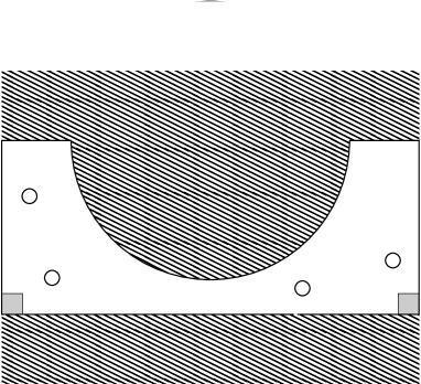
Figure 3: Sketch of the simulation box. Hard walls are marked by hatches. The remaining boundaries were treated as periodic. The grey squares mark the regions in which the density at wall contact was sampled.

III Results

III.1 Wall–solute interaction

In this section, we analyze case (a), the problem of a solute sphere close to a wall. Previous simulation work Her06 ; Her07 ; Her08 has concentrated on the particular state point $\rho_{s}^{*}=0.764$ (packing fraction $\eta_{s}=0.4$), therefore we present explicit results for the density profiles also for this state point to facilitate comparison.

III.1.1 Density profiles

In Fig. 4, we show DFT results for the solvent density profile between wall and solute for a solute–solvent size ratio of 20 and solvent–wall distance $h=0$ (i.e. contact between wall and solute molecular surface; left panel) and $h=\sigma$ (i.e. the end of the depletion region; right panel). There is strong adsorption at the apex of the annular wedge, given by the coordinates $z=0$ and $r_{||}=r_{0}=\sqrt{2R(h-\sigma)-(h-\sigma)^{2}}$, as reflected by the main peak. Along the wall ($z=0$), we observe strong structuring which is mainly dictated by packing considerations. The apex peak corresponds to a ring of solvent spheres centered at $r_{||}=r_{0}$ (for $h=0$) or just one sphere near $r_{||}=0$ (for $h=\sigma$). The second–highest peak in both panels of Fig. 4 appears where the distance between wall and solute sphere, measured along the $z$–axis, is approximately $2\sigma$ and thus two rings of spheres fit between solute and wall. However, for $h=0$ (left panel of Fig. 4) packing in $r_{||}$–direction leads to further structuring of the density profile close to the apex of the wedge.

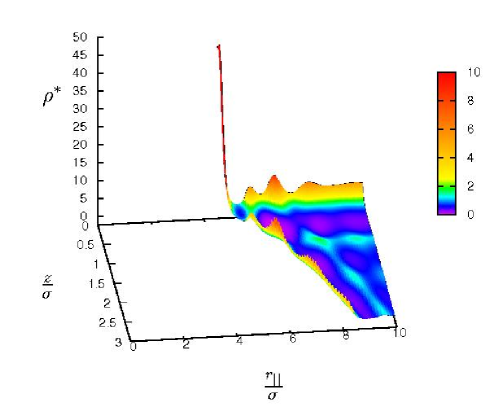
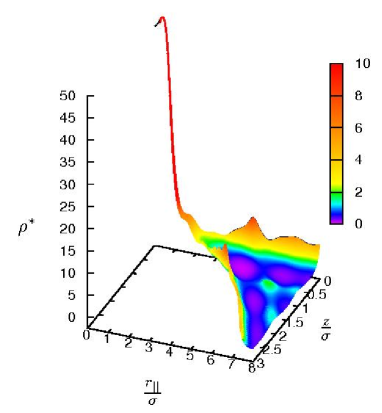
Figure 4: (color online) Density profiles from FMT–WBII of solvent spheres confined to the annular wedge between a solute sphere (size ratio $R_{b}/R_{s}=20$) and a wall. The bulk solvent density is $\rho_{s}^{*}=0.764$, and the wall separation $L=26\,\sigma$ (see Fig. 2 (a)). Grid resolution was equidistant in $z$ with $\Delta z=0.002$ $\sigma$ and equidistant in $x=\ln(r_{||}/\sigma)$ with $\Delta x=0.005$ (see App. B.2). Left panel: solute–wall distance $h=0$, right panel: $h=\sigma$.

The integral of the solvent density at the wall (i.e. the adsorption at the wall) directly determines the depletion force, see Eq. (2). Therefore, we analyze the density at the wall further. In Fig. 5 we show $\rho(r_{||},z=0)$ computed with FMT–RF, FMT–WBII, IE–MV and compare the results to the simulation data of Ref. Her07 . Overall, DFT performs quite well but it tends to overestimate the structuring of the profile. The currently most consistent version, FMT–WBII, improves over FMT–RF particularly in this respect. The integral equation results for the different closure are very similar to each other and are approximately of the same quality as the solutions of FMT–RF. Note that the simulation data of Ref. Her07 have been averaged over a distance of 0.02 $\sigma$ from the wall. This average was also applied to the DFT data (which are computed with mesh size $\Delta z=0.002\,\sigma$), whereas for the IE results we show a suitable weighted average of the zeroth and first bin ($\Delta z=0.05$), assuming linear interpolation. As seen in the right panel of Fig. 5, IE–MV gives a much lower density close to the apex of the wedge compared to the other methods. This is presumably due to the lower resolution in $z$–direction which is possible for IE (see App. C).

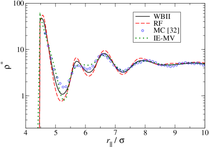
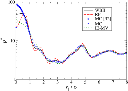
Figure 5: (color online) Comparison between the various theoretical methods and MC simulations (ours and from Ref. Her07 ) for the density at the wall (averaged over a distance of 0.02 $\sigma$). Left panel: solute–wall distance $h=0$, right panel: $h=\sigma$. The solute–solvent ratio is 20 and the solvent bulk density is $\rho_{s}^{*}=0.764$. Note the logarithmic scale on the density axis.

To further investigate the issue of the dominant packing mode in the annular wedge, we performed DFT calculations also for the additonal size ratios 10, 30, 50 and 100 for the same solvent density $\rho_{s}^{*}=0.764$. Packing in $r_{||}$–direction can be monitored conveniently by viewing the annular wedge close to the apex as a quasi–2d system (see Fig. 1 and the remarks in the Introduction). We define an effective, two–dimensional solvent density by

$$\rho_{\rm 2d}(r_{||})=\int_{0}^{z_{s}(r_{||})}dz\,\rho(r_{||},z)\;,$$ (14)

where $z_{s}(r_{||})=R-(\sigma-h)-\sqrt{R^{2}-r_{||}^{2}}\approx r_{||}^{2}/(2R)-(\sigma-h)$ defines the surface of the exclusion sphere around the solute (and thus the radius–dependent width of the annular wedge). In Fig. 6 we show results for $\rho_{\rm 2d}(r_{||})$ for two configurations with slightly different solute–wall distances: $h=0.95\,\sigma$ (left panel) and $h=\sigma$ (right panel). In the latter case, one solvent sphere fits exactly between solute and wall at the apex, nevertheless $\rho_{\rm 2d}$ vanishes there due to the vanishing slit width, $z_{s}(r_{||}\to 0)\to 0$. Note that this is also a consequence of an application of the potential distribution theorem Hen86 which states that the 3d density reaches a finite, maximum value of $\exp(\beta\mu^{ex})$ in a planar slit of vanishing width which is equivalent to a vanishing 2d density ($\mu^{ex}$ is the excess chemical potential of the bulk solvent coupled to the slit). However, when the slit widens, the 2d density quickly rises Oet04 . For $h=\sigma$ (right panel in Fig. 6), this leads to the picture of an effective 2d system with a small, soft and repulsive obstacle centered at $r_{||}=0$ which induces moderate layering in the 2d–“bulk” with an effective “bulk” density $\rho_{{\rm 2d},s}\approx 0.7\dots 0.8$. For $h=0.95\,\sigma$ (left panel in Fig. 6), the obstacle in the center has a radial extent of $r_{0}\approx\sqrt{R\sigma/10}$ which ranges from 0.75 $\sigma$ (size ratio 10) to 2.25 $\sigma$ (size ratio 100) and induces stronger layering in the effective 2d system. The oscillations occur around the same “bulk” density as in the case $h=\sigma$. The simulation results show weaker oscillations than the DFT results. Since the first peak, e. g., occurs at wedge widths $<0.03\,\sigma$, we are testing the dimensional crossover properties of DFT–FMT from 3d to 2d with a sensitive probe. The difference between the results of the simulations and the DFT versions employed here are in line with previous investigations on the dimensional crossover properties of FMT Ros97 . There it has been found that the strict 2d limit of FMT–RF results in a somewhat peculiar (integrable) divergence in the hard disk direct correlation function $c_{\rm 2d}(r)$ for $r\to 0$ and overestimated peaks in the corresponding structure factor. The tensor weight modifications introduced in Ref. Tar00 result in better dimensional crossover properties Tar02 and might improve the DFT results close to the apex of the annular wedge. A more detailed investigation of tensor–weighted FMT with regard to the correlations in narrow planar slits and also in the annular wedges considered here is certainly of interest (although the algebra of App. B becomes much more extended in this case).

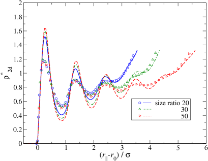
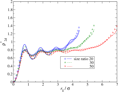
Figure 6: (color online) Effective two–dimensional solvent density in the annular wedge for various solute–solvent size ratios. Lines correspond to DFT results (FMT–WBII) and symbols show results of our MC calculations. Left panel: solute–wall distance $h=0.95\,\sigma$, right panel: $h=\sigma$. The solvent bulk density is $\rho_{s}^{*}=0.764$. The curves are plotted up to the point where the width of the annular wedge reaches the value of $\sigma$.

Our observations should be compared with the phenomenological modelling of Ref. Oet04 (“annular slit approximation”). There, the effective 2d system was approximated by an idealized system of hard disks, layering around a hard cavity of radius $r_{0}$ centered around $r_{||}=0$. The bulk density $\rho_{{\rm 2d},s}$ of this hard disk system was determined via the self–consistency condition $p_{\rm 2d}(\rho_{{\rm 2d},s})=-2\gamma(\rho_{s})$ where $p_{\rm 2d}$ is the 2d pressure and $\gamma$ is the surface tension of a hard wall immersed in a bulk solvent of density $\rho_{s}$. Employing scaled particle theory Hel61 , this yields $\rho_{{\rm 2d},s}^{*}\approx 0.66$ for $\rho_{s}^{*}=0.764$. This value is a bit smaller than the one inferred from the 2d density profiles of Fig. 6. The main difference between the idealized hard disk system of Ref. Oet04 and the effective 2d system as reflected in Fig. 6 lies probably in the softness of the central cavity obstacle and also the softness of the effective particle interactions due to the widening of the slit. Apart from that the overall picture of Ref. Oet04 is confirmed well. In particular, this implies an important observable consequence: The cavity circumference (of approximate length $2\pi r_{0}$) induces a line contribution $2\pi r_{0}\,\gamma_{\rm 2d}(\rho_{{\rm 2d},s})$ to the insertion free energy of the solute near the wall. Since the insertion free energy is equivalent to the depletion potential up to an additive constant, the latter acquires a term $\propto\sqrt{R(\sigma-h)}$, the corresponding term in the depletion force is $\propto\sqrt{R/(\sigma-h)}$. (Note that for $h\to\sigma$ the cavity radius should stay finite as reflected in Fig. 6 (right panel), thus the divergence of the depletion force there according to the geometrical argument of equating the cavity radius with $r_{0}$ is unphysical.) The interpretation of this line energy term within the more general framework of morphometric thermodynamics will be given below.

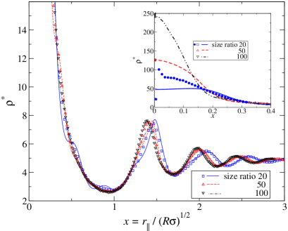
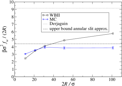
Figure 7: (color online) Left panel: density at the wall for solute–wall distance $h=\sigma$ and the three solute–solvent size ratios 20, 30 and 100. Lines are FMT–WBII data, symbols are MC simulation results from Ref. Her08 . Right panel: The depletion force between solute and wall at $h=\sigma$. The solvent bulk density is $\rho_{s}^{*}=0.764$.

We have seen that in radial direction, the packing of the solvent spheres close to the apex of the annular wedge is well understood by the quasi–2d picture developed above. For the particular point $h=\sigma$, there is only moderate layering in $r_{||}$–direction, thus the full density profile should be determined mainly by packing in $z$–direction. Indeed, for $h=\sigma$ we observe a quite remarkable collapse of the density profiles at the wall when plotted as a function of $\hat{r}=r_{||}/\sqrt{R\sigma}$, see Fig. 7, indicating the relative unimportance of packing in radial direction. According to Eq. (2), perfect scaling would imply that the depletion force at $h=\sigma$ is proportional to $R$. The DFT data violate scaling for $\hat{r}<0.2$ (i.e. when the slit width is smaller than 0.02 $\sigma$), as can be seen from Fig. 7 (left panel, inset). This leads to a slow increase of the scaled depletion force $f_{w}/(2R)$, see Fig. 7 (right panel). In contrast, the simulation results of Ref. Her08 indicate that $f_{w}/(2R)$ stays constant for large $R$, quite in agreement with an upper bound derived within the annular slit approximation of Ref. Oet04 which reads $f_{w}/(2R)=-2\pi\gamma(\rho_{s})(1-\eta_{\rm 2d})$ where $\eta_{\rm 2d}=(\pi/4)\,\rho_{{\rm 2d},s}\sigma^{2}$ is the 2d “bulk” packing fraction. Note that the value of the Derjaguin approximation at $h=\sigma$, $f_{w}/(2R)=-2\pi\gamma(\rho_{s})$ is completely off the simulation as well as the DFT values (see next subsection).

III.1.2 Geometric interpretation of the depletion force

Morphological (morphometric) thermodynamics Koe04 provides a powerful interpretation of the depletion interaction, as has been shown very recently in the special case of the solute–solute interaction Oet09 . Up to a constant, the depletion potential is nothing but the solvation free energy of the wall and the solute. In morphological thermodynamics the solvation free energy $F_{\mathrm{sol}}$ of a body is separated into geometric measures defined by its surface. As the surface, we take the solvent–accessible surface, i.e. the body surface of the combined wall–solute object is defined by the dashed lines in Fig. 2 (a). These geometric measures are the enclosed volume $V$, the surface area $A$, the integrated mean and Gaussian curvatures $C$ and $X$, respectively. To each measure there is an associated thermodynamic coefficient: the pressure $p$, the planar wall surface tension $\gamma$ and two bending rigidities $\kappa$ and $\bar{\kappa}$ such that

$$F_{\mathrm{sol}}=pV+\gamma A+\kappa C+\bar{\kappa}X.$$ (15)

Due to the separation of the solvation free energy into geometrical measures and geometry independent thermodynamic coefficients, it is possible to obtain the coefficients $p$, $\gamma$, $\kappa$ and $\bar{\kappa}$ in simple geometries. The pressure $p$ is a bulk quantity of the fluid. The surface tension $\gamma$ accounts for the free energy cost of forming an inhomogeneous density distribution close to a planar wall. If the wall is curved the additional free energy cost is measured by $\kappa$ and $\bar{\kappa}$. It is possible to obtain all four coefficients from a set of solvation free energies of a spherical particle with varying radius. For a hard-sphere solute in a hard-sphere solvent very accurate analytic expressions for the thermodynamic coefficients are known from FMT–WBII Han06 , see also App. A.

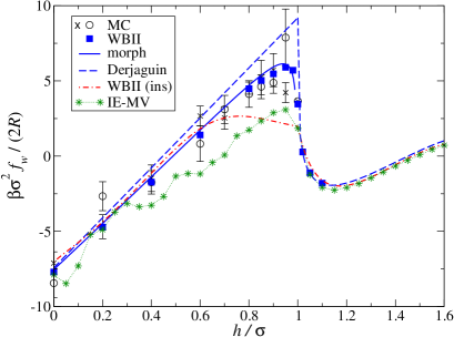
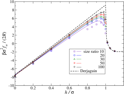
Figure 8: (color online) Depletion force between wall and solute for solvent bulk density $\rho_{s}^{*}=0.764$. Left panel: Solute–solvent size ratio 20. Simulation data are shown by crosses ($\times$) and circles (o) and differ by a slightly different choice of $\rho_{w}$ in Eq. (2) (see Refs. Her06 ; Her07 for details). Results from explicit FMT–WBII minimization are given by the full squares and results from IE–MV are shown by asterisks. The dash–dotted line shows the insertion route result using the WBII functional and the dashed line gives the Derjaguin approximation. The excess surface free energy of two parallel hard walls, needed for the Derjaguin approximation, has been calculated with the WBII functional. Right panel: depletion force for different solute–solvent size ratios. Symbols are results from explicit FMT–WBII minimization, lines in ascending order are morphometric results for size ratios 10, 20, 30, 50, 100 and $\infty$ (Derjaguin approximation).

For the particular case considered here, the depletion potential $W(h)$ follows by subtracting the sum of the solvation free energies of a single wall and a single solute sphere. Thus we find

$$W(h<\sigma) = -p\Delta V-\gamma\Delta A-\kappa\Delta C-4\pi\bar{\kappa}\;$$ (16)

where $\Delta V$ and $\Delta A$ are the volume and surface area of the overlap of the exclusion (depletion) zones around wall and solute, respectively, and $\Delta C$ is the integrated mean curvature of that overlap volume. Note that the fourth characteristic, the integrated Gaussian curvature is the Euler characteristic which is $4\pi$ for wall and solute at $h\leq\sigma$ (one connected body) and $8\pi$ for wall and solute at $h>\sigma$ (two disconnected bodies). This explains the last term in Eq. (16). The geometric measures $\Delta V$, $\Delta A$ and $\Delta C$ are given by

$$\Delta V = \frac{\pi}{3}(\sigma-h)^{2}\,(3R-(\sigma-h))$$

$$\stackrel{{\scriptstyle R\to\infty}}{{\approx}} \pi R(\sigma-h)^{2}+O(R^{0})\;,$$

$$\Delta A = 4\pi R(\sigma-h)-\pi(\sigma-h)^{2}$$ (17)

$$\stackrel{{\scriptstyle R\to\infty}}{{\approx}} 4\pi R(\sigma-h)+O(R^{0})\;,$$

$$\Delta C = 2\pi(\sigma-h)+\pi\sqrt{2R(\sigma-h)-(\sigma-h)^{2}}\left(\frac{\pi}{2}+\arcsin\left(1-\frac{\sigma-h}{R}\right)\right)$$

$$\stackrel{{\scriptstyle R\to\infty}}{{\approx}} \pi^{2}\sqrt{2R(\sigma-h)}+O(R^{0})\;.$$

The depletion force follows as $f_{w}(h)=-\partial W/\partial h$. In the limit $R\to\infty$ it is given by:

$$\frac{f_{w}(h<\sigma)}{2\pi R} \stackrel{{\scriptstyle R\to\infty}}{{\approx}} p(h-\sigma)-2\gamma-\kappa\,\frac{\pi}{2}\sqrt{\frac{1}{2R(\sigma-h)}}\;.$$ (18)

The contribution from the integrated mean curvature is subleading in $1/R$ but it is quantitatively important since it induces a singularity as $h\to\sigma$ which is proportional to $1/(\sigma-h)^{1/2}$. This contribution precisely corresponds to the line tension term associated with the circular apex (of length $2\pi r_{0}$) of the annular wedge identified in the quasi–2d analysis of Ref. Oet04 and introduced in the last subsection. The line tension in the quasi–2d picture was shown to be $\gamma_{\rm 2d}(\rho_{{\rm 2d},s})$ and in the geometric analysis it is $-\pi\kappa/2$. There is good agreement between both expressions Oet09 . Strictly, the singularity associated with this line term is unphysical of course. Indeed, it can be shown that the morphometric analysis becomes ambiguous very close to $h=\sigma$. One would require that the morphometric result for the force is unchanged if another, slightly displaced surface around the solute sphere is chosen for the geometric analysis. In Ref. Oet09 , such an analysis was carried out for the sphere–sphere geometry and the independence of the force on the chosen surface was demonstrated. However, if one chooses e.g. the molecular surface (the surface of the set of points which is never covered by a small solvent sphere), then this surface becomes self–overlapping close to $h=\sigma$ and one could not expect to ascribe physical significance to surface tensions and mean curvature coefficients of such overlapping surfaces. For the sphere–wall geometry a similar analysis holds. Note that the singularity at $h=\sigma$ corresponds to a vanishing circumference of the apex ($r_{0}=0$), however, the 2d analysis of the density distributions at this point yielded a small but finite value for the “effective” apex radius $r_{0}$ (see Fig. 6 (right panel)).

In Fig. 8 (left panel) we show FMT–WBII and IE–MV results for the depletion force $f_{w}$ between a big sphere and a wall (size ratio 20, solvent bulk density $\rho_{s}^{*}=0.764$) and compare them to MC results from Refs. Her06 ; Her07 as well as to the morphometric analysis. The force according to morphometry is plotted only until self–intersection of the molecular surface starts. The FMT data are described very well by the morphometric results; the sharp drop in the depletion force close to $h=\sigma$ appears to mimick the behavior of the singular term $\propto\partial\Delta C/\partial h$. The MC data suffer from relatively large error bars (except for the point $h=\sigma$ but are overall consistent with both the FMT data and the morphometric analysis. The scatter in the IE–MV data is due to the comparatively low resolution in $z$–direction as compared to the DFT data ($\Delta z=0.05\,\sigma$ vs. $\Delta z=0.002\,\sigma$). As before, all considered IE closures give similar results, but these correspond to an overall more attractive force compared to DFT and MC. Two other approximations for the depletion force are shown in Fig. 8 (left panel): the DFT insertion route and the Derjaguin approximation. Both approximations fail to describe the depletion force near $h=\sigma$. In the insertion route to DFT (see Ref. Rot00 for its derivation), one circumvents the explicit calculation of the density profile around the fixed wall and solute by exploiting the relation:

$$\beta W(\mathbf{x}) = \lim_{\rho_{b}\to 0}\left.\frac{\delta{\cal F}^{\rm ex}}{\delta\rho_{b}(\mathbf{x})}\right|_{\rho_{s}(\mathbf{r})=\rho_{w}(z)}-\mu^{\rm ex}_{b}(\rho_{s})\;.$$ (19)

Here, $\mu^{\rm ex}_{b}(\rho_{s})$ is the excess chemical potential for inserting one solute into the solvent with density $\rho_{s}$. The functional derivative of the mixture functional has to be evaluated in the dilute limit for the solutes, $\rho_{b}\to 0$, and with the solvent density profile given by the profile at a hard wall ($\rho_{w}(z)$). This method relies on an accurate representation of mixture effects for large size ratios in the free energy functional. Therefore, the observed deviations in the depletion force presumably follow from the insufficient representation of higher-order direct correlation functions of strongly asymmetric mixtures in the present forms of FMT Cue02 . The Derjaguin approximation, on the other hand, corresponds to the leading term for $R\to\infty$ in Eq. (18) inside the depletion region ($h<\sigma$), but is easily extended to $h\geq\sigma$ Hen02 ; Oet04 :

$$\frac{f^{\rm Derjaguin}_{w}}{2\pi R} = \left\{\begin{array}[]{lll}p(h-\sigma)-2\gamma&&(h<\sigma)\\ \gamma_{\rm slit}(h)-2\gamma&&(h\geq\sigma)\end{array}\right.\;,$$ (22)

with $\gamma_{\rm slit}(h)$ denoting the excess surface energy of two parallel hard walls at distance $h$ forming a slit. According to Eq. (2), the Derjaguin force scales with $R$ (“colloidal limit”) which is an excellent approximation outside the depletion region. (Incidentally, outside the depletion region all methods and the Derjaguin approximation agree with each other.) Inside the depletion region, the neglected mean curvature (or line tension) term is very significant.

Explicit FMT–WBII results for the depletion force for size ratios up to 100 are shown in Fig. 8 (right panel) and compared to the morphometric analysis (symbols vs. full lines). Whereas for size ratio 10 some discrepancies are still visible, they have more or less vanished for size ratio 100 (except for the point $h=\sigma$, see the previous discussion). Thus the morphometric form for the depletion force (Eq. (18)) can be regarded as the appropriate “colloidal limit”.

III.2 Solute–solute interaction

We now turn to the case of the depletion force between two big solute particles which are immersed in the hard solvent. Considering the evidence from the sphere–wall case, we would expect that for large size ratios, the morphometric picture reliably describes the depletion force. Since the geometry of the overlap volume between two spheres is different from that between a sphere and a wall, we find also a slightly different form for the morphometric force in the limit $R\to\infty$:

$$\frac{f(h<\sigma)}{\pi R} \stackrel{{\scriptstyle R\to\infty}}{{\approx}} p(h-\sigma)-2\gamma-\kappa\,\frac{\pi}{2}\sqrt{\frac{1}{R(\sigma-h)}}\;.$$ (23)

Thereby, one sees that the scaling relation $f_{w}=2f$, valid within the Derjaguin approximation, is violated through the appearance of the mean curvature (line tension) term. For moderate solvent densities up to $\rho_{s}^{*}=0.7$ the morphometric form (23) gives a good description of the depletion force for size ratios $\alpha\gtrsim 10$. This has been reported in Ref. Oet09 . An analysis of the full solvent density profiles between the two solutes reveals the same features as described in Sec. III.1.

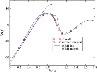
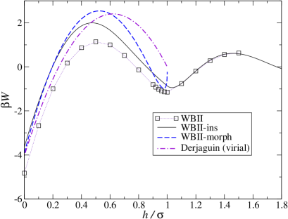
Figure 9: (color online) Left panel: Depletion force between two solutes. Circles correspond to the centered difference of the FMT-WBII data for the depletion potential (right panel), while squares give the FMT–WBII depletion force according to the surface integral in Eq. (II). Right panel: Depletion potential between two solutes. The curve for the morphometric potential has been shifted by -1. The solvent density is $\rho_{s}^{*}=0.8$ and the solute–solvent size ratio is 5.

It is interesting to investigate the regime where the morphometric description is expected to fail. This will happen when there are strong correlations in the whole annular wedge, i.e. where packing in both the $r_{||}$– and the $z$–direction becomes important. Typically, intermediate size ratios and higher solvent densities will induce these strong correlations. Therefore, we have investigated the depletion force for size ratios 5 and 10 and solvent densities $\rho_{s}^{*}=0.8$ and $\rho_{s}^{*}=0.9$. In Figs. 9 and 10 we show results for the depletion force and potential at $\rho_{s}^{*}=0.8$ for size ratios 5 and 10 respectively. For size ratio 5, the explicit DFT calculations yield a depletion force which does not correspond to the morphometric result at all. It is closer to the insertion route (see (Eq. 19)), though systematically lower. This yields a depletion potential (Fig. 9 (right panel)) which is about 1 $k_{\rm B}T$ or 25% more attractive at contact than that of the insertion route. For size ratio 10, the explicit DFT data for the depletion force reflect the morphometric form as $h\to\sigma$, i.e. they give again evidence for importance of the mean curvature (line tension) term in Eq. (23). However, away from that regime, the depletion force deviates significantly from both the morphometric form and the insertion route result such that the depletion potential at contact (Fig. 10 (right panel)) is about 3 $k_{\rm B}T$ or 50% more attractive at contact than that of the insertion route (for FMT–WBII).

Note that at such a high solvent density ($\rho_{s}^{*}=0.8$) there are already significant deviations between FMT–RF and FMT–WBII (Fig. 10 (right panel), circles and squares). Since FMT–WBII has been designed to improve thermodynamic and morphometric consistency at higher densities, the corresponding results can be assumed to be more trustworthy. As an additional check of the numerics, we calculated the depletion force in two ways: (a) via the surface integral in Eq. (II) and (b) via the centered difference of the results for the depletion potential (see Figs. 9 and 10 (left panel), squares and circles). The latter is simply obtained as

$$W(h) = \left.\Omega[\rho(\mathbf{r});h]\right|_{\rho(\mathbf{r})=\rho_{\rm eq}(r_{||},z;h)}-\left.\Omega[\rho(\mathbf{r});h\to\infty]\right|_{\rho(\mathbf{r})=\rho_{\rm eq}(r_{||},z;h\to\infty)}\;,$$ (24)

where the grand potential $\Omega$ and the equilibrium density $\rho_{\rm eq}(r_{||},z;h)$ around the two solutes at distance $h$ are determined by the basic DFT equations (3) and (5), respectively. The agreement between routes (a) and (b) is very good, save for some “fluctuations” in route (b) close to the point $h=\sigma$ where the density oscillations in the wedge are most pronounced. The equality of both routes checks a sum rule check similar to the hard wall sum rule for the problem of one wall immersed in solvent. Weighted–density DFT’s usually fulfill the latter Swo89 .

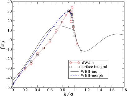
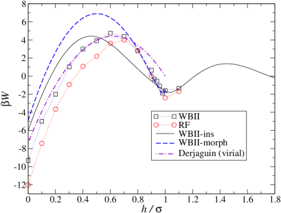
Figure 10: (color online) Left panel: Depletion force between two solutes. Circles correspond to the centered difference of the FMT-WBII data for the depletion potential (right panel), while squares give the FMT–WBII depletion force according to the surface integral in Eq. (II). Right panel: Depletion potential between two solutes. Squares correspond to FMT–WBII results, and circles to FMT–RF results. The curve for the morphometric potential has been shifted by -2. The solvent density is $\rho_{s}^{*}=0.8$ and the solute–solvent size ratio is 10.

The differences between the insertion route and the explicit FMT data becomes more dramatic for higher densities. In Fig. 11 we show results for the depletion potential for a solute–solvent size ratio 5 at solvent densities 0.85 and 0.9 (left panel) and for a size ratio 10 at density 0.85 (right panel). For size ratio 5 the repulsive barrier has almost vanished for $\rho_{s}^{*}=0.9$, and the potential well at contact is almost twice as deep as compared with the insertion route. For size ratio 10, the barrier remains (albeit at a different location) but the well depth is equally enhanced by a factor 2 compared with the insertion route as for size ratio 5.

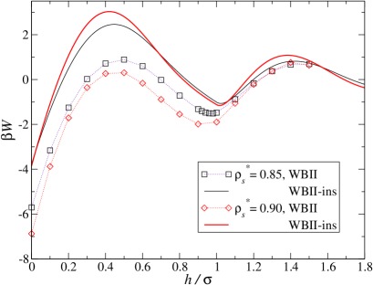
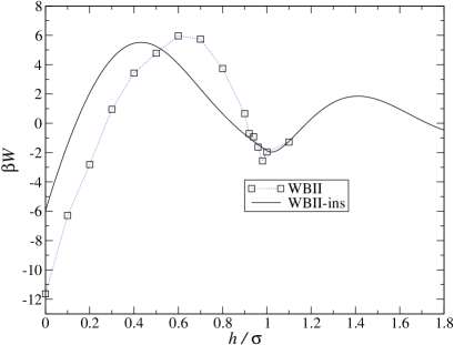
Figure 11: (color online) Depletion potential between two solutes, comparison between explicit FMT–WBII data and the insertion route. Left panel: Solute–solvent size ratio 5 and solvent densities $\rho_{s}^{*}=0.85$ and 0.9. Right panel: Size ratio 10 and $\rho_{s}^{*}=0.85$.

The significant deviations of the depletion potential (according to the explicit FMT–WBII results) from the previously known approximations (Derjaguin approximation and insertion route) sheds some doubts on the quantitative accuracy of simulations of binary hard sphere mixtures (with asymmetries between 5 and 10), employing an effective one–component approach for the solutes interacting with their depletion potential. In Ref. Dij99 the phase diagram of the mixture was scanned in that way using a virial expansion to third order in the Derjaguin approximation for the depletion potential (see the dot–dashed curves in Figs. 9 and 10 (right panel)). Especially for size ratio 5, the explicit DFT results predict a depletion potential with much smaller barrier and a deeper well at contact. This might affect the phase diagram in the corner where the packing fraction of the solutes is low and the solvent packing fraction is high. In Ref. Amo08 gellation in hard sphere–like, asymmetric mixtures is investigated with an integral equation approach (reference functional approximation Aya09 ) to the depletion potential, akin to the insertion route. We expect quantitative deviations at higher solvent densities compared to explicit DFT calculations which again affect the corner of the phase diagram with low solute and high solvent packing fraction.

Finally we want to mention that the explicit DFT methods introduced here, together with the morphometric form of the depletion force in Eq. (23), can be used to improve available analytic forms DHen08 ; DHen09 for the contact values of the pair correlation functions in hard–sphere mixtures (note that the solute–solute contact value is given by $g_{bb}(2R_{b})=\exp[-\beta W(0)]$).

IV Summary and conclusions

We have presented a detailed analysis of the relationship between depletion forces (solute–wall and solute–solute) in a hard solvent and the associated density distributions around the fixed wall/solute particles, using mainly density functional theory of fundamental measure type complemented with Monte–Carlo simulations and integral equation techniques. For large solute–solvent size ratios, the depletion force is strongly linked to the quasi two–dimensional confinement between the solutes (or the solute and the wall). We have shown that the properties of this quasi two–dimensional confined system are reflected in the depletion force by a line–tension term which in turn can be obtained quite generally through morphological thermodynamics. Thus we can formulate an appropriate “colloidal” limit for the depletion force in hard–sphere mixtures: Eq. (18) for the solute–wall case and Eq. (23) for the solute–solute case. This new formulation improves significantly over the Derjaguin approximation which is a frequently employed tool to estimate colloidal interactions in many circumstances.

Although our analysis has been restricted to hard spheres only, the formulation of morphological thermodynamics is very general such that it can be expected that the colloidal limit for the depletion force holds also in mixtures with more general interparticle interactions. However, more explicit tests in this direction are necessary.

For intermediate size ratios 5 and 10 and higher solvent densities $\rho_{s}^{*}\geq 0.8$ we found strong deviations in the solute–solute depletion force between the explicit density functional results on the one hand and the Derjaguin approximation or morphometry on the other hand. This is a result of the strong solvent correlations in the annular wedge between the solutes. The depletion well at solute contact is significantly more attractive (by almost a factor of two) than previously estimated. This might have consequences for the phase diagram of binary hard spheres at low solute and high solvent packing fractions. With recently developed techniques Mil04 ; Sch09 , this question appears to be tractable in direct simulations.

Acknowledgment: V.B., F.P. and M.O. thank the German Science Foundation for financial support through the Collaborative Research Centre (SFB–TR6) “Colloids in External Fields”, project N01. T.S. thanks the German Science Foundation for financial support through an Emmy Noether grant.

Appendix A Fundamental measure functionals for hard spheres and associated thermodynamic coefficients

We consider fundamental measure functionals involving no tensor–weighted densities which are defined by the following functional for the excess free energy of a hard sphere mixture of solvent and solute particles, described by the density distribution $\rho(\mathbf{r})=\{\rho_{s}(\mathbf{r}),\rho_{b}(\mathbf{r})\}$:

$$\beta{\cal F}^{\rm ex} = \int d\mathbf{r}\,\Phi(\{\mathbf{n}[\rho(\mathbf{r})]\})\;,$$ (25)

$$\Phi(\{\mathbf{n}[\rho(\mathbf{r})]\}) = -n_{0}\,\ln(1-n_{3})+\varphi_{1}(n_{3})\;\frac{n_{1}n_{2}-\mathbf{n}_{1}\cdot\mathbf{n}_{2}}{1-n_{3}}+\varphi_{2}(n_{3})\;\frac{n_{2}^{3}-3n_{2}\,\mathbf{n}_{2}\cdot\mathbf{n}_{2}}{24\pi(1-n_{3})^{2}}\;.$$

Here, $\Phi$, is a free energy density which is a function of a set of weighted densities $\{\mathbf{n}(\mathbf{r})\}=\{n_{0},n_{1},n_{2},n_{3},\mathbf{n}_{1},\mathbf{n}_{2}\}$ with four scalar and two vector densities. These are related to the density profile $\rho(\mathbf{r})$ by

$$n_{\alpha}=\sum_{i}\int d\mathbf{r}^{\prime}\rho_{i}(\mathbf{r}^{\prime})\,w^{\alpha}_{i}(\mathbf{r}-\mathbf{r}^{\prime})=\sum_{i}\rho_{i}*w^{\alpha}_{i}\;,$$ (26)

and the hereby introduced weight functions, $\{\mathbf{w}_{i}(\mathbf{r})\}=\{w_{i}^{0},w_{i}^{1},w_{i}^{2},w_{i}^{3},\mathbf{w}_{i}^{1},\mathbf{w}_{i}^{2}\}$, depend on the hard sphere radii $R_{i}=\{R_{s},R_{b}\}$ of the solvent and solute particles as follows:

$$w^{3}_{i}=\theta(R_{i}-|\mathbf{r}|)\;,\qquad w^{2}_{i}=\delta(R_{i}-|\mathbf{r}|)\;,\qquad w^{1}_{i}=\frac{w^{2}_{i}}{4\pi R_{i}}\;,\qquad w^{0}_{i}=\frac{w^{2}_{i}}{4\pi R_{i}^{2}}\;,$$

$$\mathbf{w}^{2}_{i}=\frac{\mathbf{r}}{|\mathbf{r}|}\delta(R_{i}-|\mathbf{r}|)\;,\qquad\mathbf{w}^{1}_{i}=\frac{\mathbf{w}^{2}_{i}}{4\pi R_{i}}\;.$$ (27)

The excess free energy functional in Eq. (25) is completed upon specification of the functions $\varphi_{1}(n_{3})$ and $\varphi_{2}(n_{3})$. With the choice

$$\varphi_{1}=1\;,\qquad\varphi_{2}=1$$ (28)

we obtain the original Rosenfeld functional Ros89 . Upon setting

$$\varphi_{1} = 1$$ (29)

$$\varphi_{2} = 1-\frac{-2n_{3}+3n_{3}^{2}-2(1-n_{3})^{2}\ln(1-n_{3})}{3n_{3}^{2}}$$

we obtain the White Bear functional Rot02 ; Yu02 , consistent with the quasi–exact Carnahan–Starling equation of state. Finally, with

$$\varphi_{1} = 1+\frac{2n_{3}-n_{3}^{2}+2(1-n_{3})\ln(1-n_{3})}{3n_{3}}$$ (30)

$$\varphi_{2} = 1-\frac{2n_{3}-3n_{3}^{2}+2n_{3}^{3}+2(1-n_{3})^{2}\ln(1-n_{3})}{3n_{3}^{2}}$$

the recently introduced White Bear II functional is recovered.

Next we briefly recapitulate the determination of the thermodynamic coefficients $p$ (pressure), $\gamma$ (hard wall surface tension), $\kappa$ and $\bar{\kappa}$ (bending rigidity of the integrated mean and Gaussian curvature, respectively) Han06 . Consider the free energy of insertion $F_{b}$ for a big solute particle of radius $R_{b}$ and associated radius $R=R_{b}+R_{s}$ of the exclusion sphere around it. According to Eq. (15), it is given by:

$$F_{b}=p\,\frac{4\pi}{3}R^{3}+\gamma\,4\pi R^{2}+\kappa\,4\pi R+\bar{\kappa}\,4\pi\;.$$ (31)

On the other hand, $F_{b}$ is equivalent to the excess chemical potential of the solutes in a mixture with solvent particles at infinite dilution ($\rho_{b}\to 0$). This excess chemical potential is obtained as the density derivative $\partial/\partial\rho_{b}$ of the mixture free energy (Eq. (25)), therefore we obtain:

$$\beta F_{b} = \lim_{\rho_{b}\to 0}\beta\frac{\partial{\cal F}^{\rm ex}}{\partial\rho_{b}}$$ (32)

$$= \frac{\partial\Phi}{\partial n_{3}}\,\frac{4\pi}{3}R_{b}^{3}+\frac{\partial\Phi}{\partial n_{2}}\,4\pi R_{b}^{2}+\frac{\partial\Phi}{\partial n_{1}}\,R_{b}+\frac{\partial\Phi}{\partial n_{0}}\>.$$

By equating the two expressions for $F_{b}$ in eqs. (31) and (32), one finds the explicit expressions for the thermodynamic coefficients as linear combinations of the partial derivatives $\partial\Phi/\partial n_{i}$. For the Rosenfeld functional, these coefficients are given by:

$$\beta p = \rho_{s}\,\frac{1+\eta_{s}+\eta_{s}^{2}}{(1-\eta_{s})^{3}}\;,$$

$$\beta\gamma = -\frac{3}{4}\rho_{s}\sigma\,\frac{\eta_{s}(1+\eta_{s})}{(1-\eta_{s})^{3}}\;,$$

$$\beta\kappa = \frac{3}{4}\rho_{s}\sigma^{2}\,\frac{\eta_{s}^{2}}{(1-\eta_{s})^{3}}\;,$$ (33)

$$\beta\bar{\kappa} = \rho_{s}\sigma^{3}\left(\frac{-2+7\eta_{s}-11\eta_{s}^{2}}{48(1-\eta_{s})^{3}}-\frac{\ln(1-\eta_{s})}{24\eta_{s}}\right)\;.$$

For the White Bear II functional, the thermodynamic coefficients have been given already in Ref. Han06 and are reproduced here for completeness:

$$\beta p = \rho_{s}\,\frac{1+\eta_{s}+\eta_{s}^{2}-\eta_{s}^{3}}{(1-\eta_{s})^{3}}\;,$$

$$\beta\gamma = -\rho_{s}\sigma\left(\frac{1+2\eta_{s}+8\eta_{s}^{2}-5\eta_{s}^{3}}{6(1-\eta_{s})^{3}}+\frac{\ln(1-\eta_{s})}{6\eta_{s}}\right)\;,$$

$$\beta\kappa = \rho_{s}\sigma^{2}\left(\frac{2-5\eta_{s}+10\eta_{s}^{2}-4\eta_{s}^{3}}{6(1-\eta_{s})^{3}}+\frac{\ln(1-\eta_{s})}{3\eta_{s}}\right)\;,$$ (34)

$$\beta\bar{\kappa} = \rho_{s}\sigma^{3}\left(\frac{-4+11\eta_{s}-13\eta_{s}^{2}+4\eta_{s}^{3}}{24(1-\eta_{s})^{3}}-\frac{\ln(1-\eta_{s})}{6\eta_{s}}\right)\;.$$

The coefficients of the White Bear II functional are remarkably consistent with respect to an explicit minimization of the functional around solutes of varying radius and fitting the corresponding insertion free energy to Eq. (31) Han06 .

Appendix B Minimization of fundamental measure functionals in cylindrical coordinates

In the following we consider a one–component fluid of solvent hard spheres only ($\rho_{s}(\mathbf{r})\equiv\rho(\mathbf{r})$). The equilibrium density profile $\rho_{\rm eq}(\mathbf{r})$ of the hard sphere fluid with chemical potential $\mu=\beta^{-1}\ln(\rho_{s}\,\Lambda^{3})+\mu^{\rm ex}$ (corresponding to the bulk density $\rho_{s}$) in the presence of an arbitrary external potential $V(\mathbf{r})$ is found by minimizing the grand potential

$$\Omega[\rho] = {\cal F}^{\rm id}[\rho]+{\cal F}^{\rm ex}[\rho]-\int d\mathbf{r}(\mu-V^{\rm ext}(\mathbf{r}))\;,$$ (35)

which leads to

$$\beta^{-1}\ln\frac{\rho_{\rm eq}(\mathbf{r})}{\rho_{s}}=-\mu[\rho_{\rm eq}(\mathbf{r})]+\mu^{\rm ex}-V^{\rm ext}(\mathbf{r})\;.$$ (36)

The functional $\mu[\rho(\mathbf{r})]$ is given by

$$\mu[\rho(\mathbf{r})] = \frac{\delta{\cal F}^{\rm ex}[\rho]}{\delta\rho(\mathbf{r})}$$ (37)

$$= \beta^{-1}\sum_{\alpha}\int d\mathbf{r}^{\prime}\,\frac{\partial\Phi}{\partial n_{\alpha}(\mathbf{r}^{\prime})}\,w^{\alpha}(\mathbf{r}^{\prime}-\mathbf{r})\;.$$ (38)

For the physical problems of this work, sphere–sphere and wall–sphere geometry, the external potential $V^{\rm ext}$ possesses rotational symmetry around the $z$–axis. Therefore we work in cylindrical coordinates $\mathbf{r}=(r_{||}\cos\phi,r_{||}\sin\phi,z)$, in which the external potential and the density profile depend only on $r_{||}$ and $z$, $V\equiv V(r_{||},z)$ and $\rho_{\rm eq}\equiv\rho_{\rm eq}(r_{||},z)$. Eqs. (36) and (38) can be solved with a standard Picard iteration procedure or a speed–enhanced scheme (see below). The technical difficulty lies in the fast and efficient numerical evaluation of the weighted densities $n_{\alpha}=\rho*w^{\alpha}$ and the convolutions $\partial\Phi/\partial n_{\alpha}*w^{\alpha}$ appearing in Eq. (38).

Convolution integrals are calculated most conveniently in Fourier space where they reduce to simple products. Generically, the (three–dimensional, 3d) Fourier transforms of the weighted densities involve a one–dimensional (1d) Fourier transform in the $z$–coordinate and a Hankel transform of zeroth or first order in the $r_{||}$–coordinate (see Sec. B.1). Both the 1d Fourier transform and the Hankel transform can be calculated using fast Fourier techniques (see Sec. B.2).

B.1 Weighted densities

The convolution integral, defining the weighted densities in Eq. (26), is calculated by:

$$\mathbf{n}(\mathbf{r})=\int\frac{d\mathbf{q}}{(2\pi)^{3}}{\exp(-i\mathbf{q}\cdot\mathbf{r})}\,\tilde{\rho}(q_{||},q_{z})\,\tilde{\mathbf{w}}(\mathbf{q})\;.$$ (39)

The 3d Fourier transform of the density profile $\rho(r_{||},z)$ appearing in the above equation is given by:

$$\tilde{\rho}(q_{||},q_{z}) = \int d\mathbf{r}\exp(i\mathbf{q}\cdot\mathbf{r})\rho(r_{||},z)\;$$ (40)

$$= \int_{-\infty}^{\infty}dz\,\exp(iq_{z}z)\,\int_{0}^{\infty}2\pi r_{||}dr_{||}\,J_{0}(q_{||}r_{||})\,\rho(r_{||},z)\;,$$ (41)

$$= {\rm FT}\;{\rm HT}_{0}\;\rho(r_{||},z)\;.$$ (42)

Here, we have introduced shorthand notations ${\rm FT}\;$ for the Fourier transform in the $z$–coordinate and ${\rm HT}_{i}\;$ for the Hankel transform in the $r_{||}$–coordinate involving the kernel $J_{i}(q_{||}r_{||})$. A vector in real space is given by $\mathbf{r}=r_{||}\mathbf{e}_{||}+z\mathbf{e}_{z}$, whereas a vector in Fourier space is given by $\mathbf{q}=q_{||}\mathbf{e}^{\prime}_{||}+q_{z}\mathbf{e}_{z}$, with $\mathbf{e}_{||}\cdot\mathbf{e}^{\prime}_{||}=\cos\phi_{q}$. The 3d Fourier transforms $\tilde{\mathbf{w}}$ of the set of weight functions $\mathbf{w}$ reduce to sine transforms due to radial symmetry and are explicitly given by

$$\tilde{w}^{3}(q) = \frac{4\pi R}{q^{2}}\left(\frac{\sin(qR)}{qR}-\cos(qR)\right)\;,$$ (43)

$$\tilde{w}^{2}(q) = \frac{4\pi R}{q}\,\sin(qR)\;,$$ (44)

$$\tilde{\mathbf{w}}^{2}(\mathbf{q}) = -i\mathbf{q}\,\tilde{w}^{3}(q)$$ (45)

(The remaining weighted densities differ only by a multiplicative factor.) It is convenient to introduce the following parallel and perpendicular components of the Fourier transformed vector weights ($k=1,2$):

$$\tilde{w}^{k}_{||} = i\mathbf{e}^{\prime}_{||}\cdot\tilde{\mathbf{w}}^{k}(\mathbf{q})\;,$$ (47)

$$\tilde{w}^{k}_{z} = i\mathbf{e}_{z}\cdot\tilde{\mathbf{w}}^{k}(\mathbf{q})\;.$$ (48)

Using these definitions, the scalar weighted densities are given by

$$n_{k}(r_{||},z)={\rm FT}\;^{-1}{\rm HT}_{0}\;^{-1}\left[\tilde{\rho}(q_{||},q_{z})\;\tilde{w}^{k}\left(\sqrt{q_{||}^{2}+q_{z}^{2}}\right)\right]\;.\qquad(k=0\dots 3)\;.$$ (49)

The vector weighted densities, on the other hand, are given by two components ($k=1,2$):

$$\mathbf{n}_{k}(\mathbf{r}) = n_{k,||}(r_{||},z)\mathbf{e}_{||}+n_{k,z}(r_{||},z)\mathbf{e}_{z}\;,$$

$$n_{k,||}(r_{||},z) = -{\rm FT}\;^{-1}{\rm HT}_{1}\;^{-1}\left[\tilde{\rho}(q_{||},q_{z})\;\tilde{w}^{k}_{||}(q_{||},q_{z})\right]\;,$$ (50)

$$n_{k,z}(r_{||},z) = {\rm FT}\;^{-1}{\rm HT}_{0}\;^{-1}\left[\tilde{\rho}(q_{||},q_{z})\;(-i)\tilde{w}^{k}_{z}(q_{||},q_{z})\right]\;.$$

We demonstrate this result for the example of the weighted density $\mathbf{n}_{2}$. Upon choosing $\mathbf{r}=(r_{||},0,z)$ we find

$$\mathbf{n}_{2}(\mathbf{r}) = \int\frac{d\mathbf{q}}{(2\pi)^{3}}{\exp(-i\mathbf{q}\cdot\mathbf{r})}\;\tilde{\rho}(q_{||},z)\,(-i\mathbf{q})\tilde{w}^{3}(q)\;,$$

$$= \int_{-\infty}^{\infty}\frac{dq_{z}}{(2\pi)^{3}}\,\exp(-iq_{z}z)\int_{0}^{\infty}q_{||}dq_{||}\,\tilde{\rho}(q_{||},z)\int_{0}^{2\pi}d\phi_{q}\,\exp(-iq_{||}r_{||}\cos\phi_{q})\left(\begin{matrix}-i\tilde{w}^{2}_{||}\cos\phi_{q}\\ -i\tilde{w}^{2}_{||}\sin\phi_{q}\\ -i\tilde{w}^{2}_{z}\end{matrix}\right)$$

$$= \int_{-\infty}^{\infty}\frac{dq_{z}}{2\pi}\,\exp(-iq_{z}z)\int_{0}^{\infty}\frac{q_{||}dq_{||}}{2\pi}\,\tilde{\rho}(q_{||},z)\left(\begin{matrix}-J_{1}(q_{||}r_{||})\tilde{w}^{2}_{||}\\ 0\\ -iJ_{0}(q_{||}r_{||})\tilde{w}^{2}_{z}\end{matrix}\right)\;,$$ (52)

which is equivalent to Eq. (50) for $k=2$. Here we made use of the integrals

$$\int_{0}^{2\pi}d\phi\exp(-ix\cos\phi) = 2\pi J_{0}(x)\;,$$

$$\int_{0}^{2\pi}d\phi\exp(-ix\cos\phi)\sin\phi = 0\;,$$

$$\int_{0}^{2\pi}d\phi\exp(-ix\cos\phi)\cos\phi = 2\pi iJ_{0}^{\prime}(x)=-2\pi iJ_{1}(x)\;.$$

Next we consider the evaluation of the convolution type integrals appearing in $\mu[\rho]$ (see Eq. (38)):

$$\mu[\rho]=\sum_{\alpha}\int d\mathbf{r}^{\prime}p_{\alpha}(\mathbf{r}^{\prime})w^{\alpha}(\mathbf{r}^{\prime}-\mathbf{r})\;,$$ (53)

where $p_{\alpha}=\partial\Phi/\partial n_{\alpha}$ and $\alpha$ runs over scalar and vector indices. For scalar indices, $w^{k}(\mathbf{r})=w^{k}(-\mathbf{r})$: we recover the standard convolution integral and thus:

$$\int d\mathbf{r}^{\prime}p_{k}(\mathbf{r}^{\prime})w^{k}(\mathbf{r}^{\prime}-\mathbf{r})={\rm FT}\;^{-1}{\rm HT}_{0}\;^{-1}\left[\tilde{p}_{k}(q_{||},q_{z})\;\tilde{w}^{k}\left(\sqrt{q_{||}^{2}+q_{z}^{2}}\right)\right]\qquad(k=0\dots 3)\;.\quad$$ (54)

In the case of vector indices, we observe that the free energy density $\Phi$ only depends on vector densities through $\mathbf{n}_{1}\cdot\mathbf{n}_{2}$ and $\mathbf{n}_{2}\cdot\mathbf{n}_{2}$. Thus we find ($k=1,2$):

$$\mathbf{p}_{k}(\mathbf{r}) = p_{k,||}(r_{||},z)\mathbf{e}_{||}+p_{k,z}(r_{||},z)\mathbf{e}_{z}\quad\to$$ (55)

$$\tilde{\mathbf{p}}_{k}(\mathbf{q}) = \tilde{p}_{k,||}(q_{||},q_{z})\mathbf{e}^{\prime}_{||}+\tilde{p}_{k,z}(q_{||},q_{z})\mathbf{e}_{z}$$ (56)

with

$$\tilde{p}_{k,||}(q_{||},q_{z})=i\,{\rm FT}\;{\rm HT}_{1}\;p_{k,||}(r_{||},z)\;,\qquad\tilde{p}_{k,z}(q_{||},q_{z})={\rm FT}\;{\rm HT}_{0}\;p_{k,z}(r_{||},z)\;.$$ (57)

Therefore the vector part summands of $\mu[\rho]$ are evaluated by

$$\int d\mathbf{r}^{\prime}p_{k}(\mathbf{r}^{\prime})\mathbf{w}^{k}(\mathbf{r}^{\prime}-\mathbf{r})={\rm FT}\;^{-1}{\rm HT}_{0}\;^{-1}\left[-\tilde{p}_{k,||}\tilde{w}^{k}_{||}+i\tilde{p}_{k,z}\tilde{w}^{k}_{z}\right]$$ (58)

B.2 Fast Hankel transforms

Hankel transforms can be calculated by employing fast Fourier transforms on a logarithmic grid. Consider the Hankel transform

$${\rm HT}_{\mu}\;f(r_{||}) = 2\pi\int_{0}^{\infty}r_{||}dr_{||}\,J_{\mu}(q_{||}r_{||})\,f(r_{||})\;.$$ (59)

We define new variables $x=\ln(r_{||}/r_{0})$ and $y=\ln(q_{||}/q_{0})$ with arbitrary constants $r_{0}$ and $q_{0}$. In terms of these variables

$${\rm HT}_{\mu}\;f(r_{||}) = 2\pi r_{0}^{2}\int_{-\infty}^{\infty}dx\,\hat{J}_{\mu}(x+y)\,\hat{f}(x)\;,$$ (60)

where $\hat{J}_{\mu}(x)=J_{\mu}(q_{0}r_{0}e^{x})$ and $\hat{f}(x)=e^{2x}f(e^{x})$. Thus, the Hankel transform takes the appearance of a cross–correlation integral and can be solved via Fourier transforms:

$${\rm HT}_{\mu}\;f(r_{||}) = 2\pi r_{0}^{2}\;{\rm FT}\;^{-1}\left[{\rm FT}\;\hat{J}_{\mu}(x)\,{\rm FT}\;^{\!\!*}\hat{f}(x)\right]\;.$$ (61)

The Fourier transform of $\hat{J}_{\mu}$ can be done analytically while the remaining ones are computed numerically using Fast Fourier techniques.

In the actual implementation we followed Ref. Ham00 which details the proof of orthonormality for discrete functions, defined on a finite interval in logarithmic space (and continued periodically). The following remarks apply:

• The fast Hankel transform cannot be applied directly to the density profile, $f(r_{||})\equiv\rho(r_{||},z)$, since it does not go to zero for $r_{||}\to\infty$. It is therefore advantageous to split the external potential

  $$V^{\rm ext}(\mathbf{r})=V(z)+V_{s}(r_{||},z)$$ (62)

  into a (possibly) $z$–dependent background part $V(z)$ and the remainder. The corresponding background profile $\rho_{V}$ fulfills

  $$\ln\frac{\rho_{V}(z)}{\rho_{s}}=-\beta\mu[\rho_{V}(z)]+\beta\mu^{\rm ex}-\beta V(z)\;.$$ (63)

  The full equilibrium profile can then be written as $\rho_{\rm eq}(r_{||},z)=\rho_{V}(z)(h(r_{||},z)+1)$ with $h(r_{||},z)\to 0$ for $r_{||}\to\infty$. The determining equation for $h$ reads

  $$\ln(h(r_{||},z)+1)=-\beta\mu[\rho_{V}(z)h(r_{||},z)+\rho_{V}(z)]+\beta\mu[\rho_{V}(z)]-\beta V_{s}(z)\;.$$ (64)

  Thus one needs to perform Hankel transforms only on functions which properly go to zero for $r_{||}\to\infty$. In the wall–sphere case, $V(z)$ is naturally given by the wall potential, $V_{s}$ becomes the solute–solvent pair potential $u_{bs}$ and $h\equiv h_{bs}$ is the solute–solvent pair correlation function. In that form, Eq. (64) resembles the general closure for integral equations (Eq. (10)). In the sphere–sphere case, $V(z)=0$ with $\rho_{V}=\rho_{s}$.

• The assumed periodicity of $\hat{f}(x)$ leads to restrictions on the product $q_{0}r_{0}$ (low–ringing condition in Ref. Ham00 ). This condition cannot be fulfilled on one grid for both ${\rm HT}_{0}\;(\cdot)$ and ${\rm HT}_{1}\;(\cdot)$. However, this does not lead to any noticeable instabilities in the repeated application of the fast Hankel transform.

• In order to avoid aliasing and the amplification of numerical “noise” in the low–$x$ and high–$x$ tails of $\hat{f}(x)$ in the repeated application of the fast Hankel transform we worked with cutoffs $r_{\rm min}/r_{0}=q_{\rm min}/q_{0}=0.01$ and $r_{\rm max}/r_{0}=q_{\rm max}/q_{0}=O(100)$. The fast Hankel transform itself was calculated on an extended grid $x\in[-N_{||}\Delta x/2,N_{||}\Delta x/2]$ with either $N_{||}=2048,\Delta x=0.01$ or $N_{||}=4096,\Delta x=0.005$. Outside the “physical” domain defined by $x_{\rm phys}\in[\ln(r_{\rm min}/r_{0}),\ln(r_{\rm max}/r_{0})]$ the function $\hat{f}(x)$ was put to zero (a similar prescription applies to $y_{\rm phys}$).

B.3 Speedup of iterations

The density profile $\rho(r_{||},z)$, the weighted densities $\mathbf{n}(r_{||},z)$ and the derivatives $\mathbf{p}(r_{||},z)=\partial\Phi/\partial\mathbf{n}(r_{||},z)$ have been discretized on a two–dimensional grid spanning the plane $(r_{||},z)$. Spacing in $z$–direction was equidistant with grid width $\Delta z=0.002\dots 0.005\sigma$ with up to $N_{z}=15,000$ points. Spacing in $r_{||}$–direction was logarithmic (see above) with $N_{||}\approx 1,000\dots 2,000$ points. Memory requirement went up to 16 GB for the largest grids. Computations have been performed on nodes with 16 GB RAM and two Intel QuadCore processors, with OpenMP parallelization of the arrays of Fourier and Hankel transforms. One evaluation of $\mu[\rho]$ (one iteration) took up to two minutes.

The equilibrium density profile fulfilling Eq. (36) or Eqs. (63) and (64) can be determined by Picard iterations where, as a minimum requirement for convergence, careful mixing of the current and previous iteration is necessary. However, for packing fractions $\eta>0.3$ and larger colloid–solvent size ratios $\alpha>5$ one easily needs several hundreds to thousands of iterations until convergence. In view of the iteration times up to two minutes, this is inacceptable. Therefore we employed the modified DIIS (direct inversion in iterative subspace) scheme developed in Ref. Kov99 which essentially constructs the next iterative step out of a certain number of previous steps. In the DIIS scheme, the mixing coefficients of the previous steps, determining the solution of the next step, are obtained by a minimization condition on the residual. The modification to DIIS consists in the admixture of the extrapolated DIIS residual to the solution of the next iterative step, in order to enlarge the dimensionality of the iterative subspace and thus to reach the true solution much more quickly. Our practical experience with modified DIIS is very similar to the observations in Ref. Kov99 , this includes the necessity to combine DIIS with Picard steps carefully, in case the DIIS steps show divergent behaviour. In summary, modified DIIS is a robust method for our problem, and the total number of iterations is reduced to approximately 100 and less for most parameter choices. The only noticeable exception occured for the case of the nearly singular annular wedge, i.e. when the distance $h$ between wall and colloidal sphere (or the two colloidal spheres) is $\approx 1\,\sigma$ and the solvent packing fraction $\eta_{s}>0.35$. Here, several hundred of intermediate Picard steps between two DIIS steps where occasionally necessary to prepare the ground for the next DIIS step.

Appendix C Integral equations for the solute–wall case: Numerical solution

In cylindrical coordinates the inhomogeneous OZ equations (7)–(8) read

$$h_{ss}(z,z_{0},s)-c_{ss}(z,z_{0},s) = \int d\mathbf{s}^{\prime}dz^{\prime}\rho_{V}(z^{\prime})h_{ss}(z,z^{\prime},|\mathbf{s}-\mathbf{s}^{\prime}|)c_{ss}(z^{\prime},z_{0},s^{\prime})\;,$$ (65)

$$h_{bs}(z,z_{0},s)-c_{bs}(z,z_{0},s) = \int d\mathbf{s}^{\prime}dz^{\prime}\rho_{V}(z^{\prime})h_{bs}(z,z^{\prime},|\mathbf{s}-\mathbf{s}^{\prime}|)c_{ss}(z^{\prime},z_{0},s^{\prime})\;,$$ (66)

where the total and direct correlation functions $h_{ij}(z,z_{0},s)$ and $c_{ij}(z,z_{0},s)$ of two particles depend on the distances $z$ and $z_{0}$ from the wall and on the projection of their position vectors on the direction along the wall, $\mathbf{s}=\mathbf{r}_{||}-\mathbf{r}_{||,0}$. The integral over $\mathbf{s}^{\prime}$ is a 2D convolution, which is most efficiently done by means of the Fast Hankel transform of the zeroth-order (see Appendix B.2). In Fourier space, the OZ equations become

$$\tilde{h}_{ij}(z,z_{0},q_{||})-\tilde{c}_{ij}(z,z_{0},q_{||})=\sum_{k=b,s}\int dz^{\prime}\rho_{V,k}(z^{\prime})\tilde{h}_{ik}(z,z^{\prime},q_{||})\tilde{c}_{kj}(z^{\prime},z_{0},q_{||})\;,$$ (67)

where $\tilde{h}[c](z,z_{0},q_{||})={\rm HT}_{0}\;h[c](z,z_{0},r_{||})$. The remaining $z$-integral is evaluated with a simple trapezoidal rule on a uniformly discretized grid of $N_{z}$ points, yielding the following matrix equation:

$$\mathbf{H}_{ij}(q_{||})-\mathbf{C}_{ij}(q_{||})=\sum_{k=b,s}\mathbf{H}_{ik}(q_{||})\mathit{\mathbf{R}}\mathbf{C}_{kj}(q_{||})\;,$$ (68)

where $\mathbf{H}$ and $\mathbf{C}$ are $N_{z}\times N_{z}$ matrices generated by the corresponding correlation functions at each $q_{||}$ point and $\mathit{\mathbf{R}}$ is a diagonal matrix corresponding to $\rho_{V}(z)\delta(z-z^{\prime})$.

The Lovett–Mou–Buff–Wertheim (LMBW) equation (9) for the background density profile in the presence of a hard wall takes the following form:

$$\frac{\partial\rho_{V}(z)}{\partial z}=\rho_{V}(z)\left(\rho_{V}(0)\int d\mathbf{r_{||}}c_{ss}(z,0,r_{||})+\int dz^{\prime}d\mathbf{r_{||}}c_{ss}(z,z^{\prime},r_{||})\frac{\partial\rho_{V}(z^{\prime})}{\partial z^{\prime}}\right)\;.$$ (69)

Here the 2D integration over $r_{||}$ can be considered as the DC component $q_{||}=0$ of the Hankel transform of the direct correlation function $\tilde{c}_{ss}(z,z^{\prime},q_{||})$ and the remaining integral in the second term is taken again with the trapezoidal rule. Note, that the contact density at the plannar wall is known exactly from the wall theorem $\rho_{V}(0)=\beta p$, where $p$ is the bulk pressure Henderson80 . Thus, a substitution of the contact density by the expression for the bulk pressure provides the modified LMBW equation for the density profile Quintana89 . Following the ansatz of Plischke and Henderson Plischke90 , we used the Carnahan-Starling fit for pressure, which is the first equation in (34). This in general should improve the accuracy of the density profiles near a plannar wall, if an approximation to the solvent direct correlation function $c_{ss}(z,z^{\prime},r_{||})$ is applied.

The closure equation (10) is the central one in the elaboration of a successful theory, since the OZ and LMBW equations described above are formally exact and need to be complemented with a third relation between between correlation total and direct functions. Unfortunately, in its exact form this third relation, expressed via additional bridge function $b_{ij}(\mathbf{r},\mathbf{r}_{0})$ is defined only as an infinite sum of highly connected bridge diagrams and so cannot be fully utilized. In practice, one needs to resort to different approximations, which are suited for particular applications depending on the system state. We considered the Percus–Yevick (PY), Rogers–Young (RY) and modified Verlet (MV) closures defined in Eqs. (11)–(13). For RY we use a scaled one–parameter form for $\xi_{ij}$, $\xi_{ij}=\xi/(R_{i}+R_{j})$ with $\xi=0.160$ to fulfill the single–component thermodynamic consistency requirement. For $\xi=0$ one recovers the PY closure (Eq.(11)), while for $\xi\rightarrow\infty$ one obtains the HNC closure. Likewise the HNC closure is recovered if $\alpha_{ij}\to\infty$ in the MV closure (Eq. (13)). MV is consistent with PY up to the fourth virial coefficient, if the $\alpha_{ij}$ are density independent. Here we follow the suggestion of Henderson et. al. Henderson96 and use their definition for the state–dependent parameters $\alpha_{ij}$. In the infinite dilution limit considered in the present paper these parameters reduce to the one–component form

$$\alpha=\frac{17}{120\eta_{s}}\exp(-2^{\eta_{s}})+0.8-0.45\eta_{s}\;.$$

The contact values from the MV closure proved to be in good agreement with the values calculated from Carnahan–Starling equation of state, which constitutes a considerable improvement over the PY and HNC approximations.

In the application of these closures to the inhomogeneous system the following precautions must be observed to obtain robust results.

• Technically we use the same iteration scheme as in Sec. B.3 for the numerical solution of Eqs. (68)-(69) and (10) (though due to the memory restrictions the $z$–grid spacing was only $\Delta z=0.05\sigma$ with up to $N_{z}=400$ points). The convergence drastically depends on the initial conditions, i.e. the zeroth iteration. While solving the PY closure it was enough to initialize both solvent–solvent and solute–solvent correlation functions with zeros, the RY and MV solute–solvent correlations have to be initialized with a good guess to the final solution (which was actually the corresponding PY result). The LMBW equation imposes even stronger requirement on the initial profile, which needs to be either close to the true profile or evolve very slowly from the flat profile together with the corresponding correlation functions.

• It turned out that the order of iterations is crucial for the overall convergency: for a given approximation to the density profile one needs to solve the closure and OZ equations prior to the next iteration on the LMBW equation. It is therefore very costly to get a fully self–consistent solution of all three equations and normally the convergence goal for the background density $\rho_{V}(z)$ is much lower than for the correlation functions.

• To avoid the necessity of requiring the bulk equilibrium behavior in correlation functions for distances far enough from the hard wall, we introduced the second wall at $L\sim 20\sigma$ apart from the first one. The wide slit geometry allowed us to keep the $z$–resolution at the maximal possible, yet feasible level. Finer resolution in $z$ in general improves numerical stability of the iteration procedure. Alternatively, one can use a very recent method of the expansion into the orthogonal set of functions proposed by Lado in Ref. Lado09 .

References

- (1) T. Morita and K. Hiroike, Prog. Theor. Phys 23, 1003 (1960).
- (2) G. Stell, in The Equilibrium Theory of Classical Fluids edited by H. L. Frisch J. L. Lebowitz (Benjamin, New York 1964) p. II-171.
- (3) Y. Rosenfeld, Phys. Rev. Lett. 63, 980 (1989).
- (4) R. Roth, R. Evans, A. Lang, and G. Kahl, J. Phys.: Cond. Matt. 14, 12063 (2002).
- (5) Y.-X. Yu and J. Wu, J. Chem. Phys. 117, 10156 (2002).
- (6) H. Hansen–Goos and R. Roth, J. Phys.: Condens. Matter 18, 8413 (2006).
- (7) A. Malijevsky, J. Chem. Phys. 125, 194519 (2006).
- (8) H. Hansen–Goos and K. Mecke, Phys. Rev. Lett. accepted (2009).
- (9) D. Pini and G. Stell, Physica A 306, 270 (2002).
- (10) A. Parola, D. Pini, and L. Reatto, Phys. Rev. Lett. 100, 165704 (2008).
- (11) A. Ayadim, M. Oettel, and S. Amokrane, J. Phys.: Condens. Matter 21, 115103 (2009).
- (12) Yu. Trukhina and T. Schilling, Phys. Rev. E 77, 011701 (2008).
- (13) S. Jungblut, K. Binder, and T. Schilling, J. Phys.: Condens. Matter 20, 404223 (2008).
- (14) J. Israelachvili, Intermolecular and Surface Forces, 2nd ed. (Academic Press, London 1991).
- (15) R. P. A. Dullens, Soft Matter 2, 805 (2006).
- (16) C. Likos, Phys. Rep. 348, 267 (2001).
- (17) W. G. McMillan and J. E. Mayer, J. Chem. Phys. 13, 276 (1945).
- (18) M. Dijkstra M, R. van Roij, and R. Evans, Phys. Rev. E 59, 5744 (1999).
- (19) P. Attard and G. N. Patey, J. Chem. Phys. 92, 4970 (1990).
- (20) R. Roth, R. Evans, and S. Dietrich, Phys. Rev. E 62, 5360 (2000).
- (21) S. Amokrane and J. G. Malherbe, J. Phys.: Condens. Matter 13, 7199 (2001).
- (22) A. Ayadim A, J. G. Malherbe, and S. Amokrane, J. Chem. Phys. 122, 234908 (2005).
- (23) S. Amokrane, A. Ayadim, and J. G. Malherbe, J. Phys. Chem. C 111, 15982 (2007).
- (24) B. V. Derjaguin, Kolloid Zeitschrift 69, 155 (1934).
- (25) J. R. Henderson, Physica A 313, 321 (2002).
- (26) M. Oettel, Phys. Rev. E 69, 041404 (2004).
- (27) T. Biben, P. Bladon, and D. Frenkel, J. Phys.: Cond. Matt. 8, 10799 (1996).
- (28) R. Dickman, P. Attard, and V. Simonian, J. Chem. Phys. 107, 205 (1997).
- (29) M. Oettel, H. Hansen–Goos, P. Bryk, and R. Roth, EPL 85, 36003 (2009).
- (30) P.-M. König, R. Roth R. and K. Mecke, Phys. Rev. Lett. 93, 160601 (2004).
- (31) A. R. Herring and J. R. Henderson, Phys. Rev. Lett. 97, 148302 (2006).
- (32) A. R. Herring and J. R. Henderson, Phys. Rev. E 75, 011402 (2007).
- (33) A. Herring, Ph.D. Thesis, University of Leeds (2008).
- (34) P. Tarazona, Phys. Rev. Lett. 84, 694 (2000).
- (35) P. Tarazona and Y. Rosenfeld, Phys. Rev. E(R) 55, 4873 (1997).
- (36) Y. Rosenfeld, M. Schmidt, H. Löwen, and P. Tarazona, Phys. Rev. E 55, 4245 (1997).
- (37) A. J. Archer, R. Evans, R. Roth, and M. Oettel, J. Chem. Phys. 122, 084513 (2005).
- (38) S. Egorov, Phys. Rev. E 70, 031402 (2004).
- (39) D. Goulding and S. Melchionna, Phys. Rev. E 64, 011403 (2001).
- (40) P. Tarazona, Mol. Phys. 52, 847 (1984).
- (41) K. Hillebrand, and R. M. Nieminen Surf. Sci. 147, 599 (1984).
- (42) E. Bruno, C. Caccamo, and P. Tarazona, Phys. Rev. A 35, 1210 (1987).
- (43) M. Plischke and D. Henderson, J. Chem. Phys. 84, 2846 (1986).
- (44) R. Kjellander and S. Sarman, Chem. Phys. Lett. 149, 102 (1988).
- (45) R. Kjellander and S. Sarman, Mol. Phys. 70, 215 (1990).
- (46) R. Kjellander and S. Sarman, Mol. Phys. 74, 665 (1991).
- (47) R. Lovett, C. Y. Mou, and F. P. Buff, J. Chem. Phys. 65, 570 (1976); M. Wertheim, ibid,65, 2377 (1976).
- (48) J.–P. Hansen and I. R. McDonald, Theory of simple liquids (Academic Press, London 2006).
- (49) F. Lado, S. M. Foiles, and N. W. Ashcroft, Phys. Rev. A 28, 2374 (1983).
- (50) J. L. Lebowitz, Phys. Rev. 133, A895 (1964).
- (51) F. J. Rogers, and D. A. Young, Phys. Rev. A 30, 999 (1984).
- (52) D. Henderson, A. Malijevsky, S. Labik, and K. Y. Chan, Mol. Phys. 87, 273 (1996).
- (53) P. Attard, J. Chem. Phys 91, 3072 (1989); J. Chem. Phys 91, 3083 (1989).
- (54) J. R. Henderson, Mol. Phys. 59, 89 (1986).
- (55) E. Helfand, H. L. Frisch, and J. L. Lebowitz, J. Chem. Phys. 34, 1037 (1961).
- (56) P. Tarazona, Physica A 306, 243 (2002).
- (57) J. A. Cuesta, Y. Martinez–Raton, and P. Tarazona, J. Phys.: Condens. Matter 14, 11965 (2002).
- (58) F. van Swol and J. R. Henderson, Phys. Rev. A 40, 2567 (1989).
- (59) Ph. Germain and S. Amokrane, preprint arXiv:0811.2707 (2008).
- (60) M. Alawneh, and D. Henderson, Mol. Phys. 106, 607 (2008).
- (61) A. Santos, S. B. Yuste, M. Lopez de Haro, M. Alawneh, and D. Henderson, preprint arXiv:0902.0683 (2009).
- (62) M. Miller and D. Baxter, J. Chem. Pys. 121, 535 (2004).
- (63) J. Schwarz–Linek, A. Winkler, N. Pham, T. Schilling, and W. C. K. Poon, Aggregation in Escherichia coli suspensions induced by anionic polyelectrolytes, preprint (2009).
- (64) A. J. S. Hamilton, Mon. Not. Roy. Astron. Soc. 312, 257 (2000).
- (65) A. Kovalenko, S. Ten–No, and F. Hirata, J. Comp. Chem. 20, 928 (1999).
- (66) D. Henderson, J. L. Lebowitz, L. Blum, and E. Waisman, Mol. Phys. 39, 47 (1980).
- (67) J. Quintana, D. Henderson and M. Plischke, J. Chem. Phys. 93, 4304 (1989).
- (68) M. Plischke and D. Henderson, J. Chem. Phys. 93, 4489 (1990).
- (69) F. Lado. Mol. Phys. 107, 1 (2009).