Kinematics of the Orion Nebula Cluster: Velocity Substructure and Spectroscopic Binaries

Abstract

We present a kinematic study of the Orion Nebula Cluster based upon radial velocities measured by multi-fiber echelle spectroscopy at the 6.5 meter MMT and Magellan telescopes. Velocities are reported for 1613 stars, with multi-epoch data for 727 objects as part of our continuing effort to detect and analyze spectroscopic binaries. We confirm and extend the results of Furesz et al. showing that the ONC is not relaxed, consistent with its youth, and that the stars generally follow the position-velocity structure of the moderate density gas in the region, traced by ¹³CO. The additional radial velocities we have measured enable us to probe some discrepancies between stellar and gaseous structure which can be attributed to binary motion and the inclusion of non-members in our kinematic sample. Our multi-epoch data allow us to identify 89 spectroscopic binaries; more will be found as we continue monitoring. Our results reinforce the idea that the ONC is a cluster in formation, and thus provides a valuable testing ground for theory. In particular, our observations are not consistent with the quasi-equilibrium or slow contraction models of cluster formation, but are consistent with cold collapse models.

1 Introduction

Observational evidence accumulated over the last decade has shown that most stars form in clusters (Carpenter, 2000; Lada & Lada, 2003; Allen et al., 2007). Therefore, understanding cluster formation is an important aspect of star formation theory. Cluster origin theories range from highly dynamic models (Bonnell et al., 2003) to quasi-equilibrium and/or slow contraction scenarios (Tan et al., 2006). Observations of very young clusters, before they have dynamically relaxed, can provide indications of initial conditions of formation and thus constraints on theories of cluster formation.

The Orion Nebula Cluster (ONC) is the nearest young cluster of substantial size, with approximately 2000 $M_{\sun}$ of stars within 2 pc of the Trapezium (Hillenbrand & Hartmann, 1998, HH98). Although HH98 were able to fit a King cluster model to the azimuthally-averaged spatial distribution of the stars, they suggested that the ONC may not be fully relaxed. Also, they pointed out that the cluster becomes increasingly elongated on larger scales, in the direction of the filamentary molecular gas in the region. Scally et al. (2005) emphasized the elongated nature of the stellar distribution on large scales and pointed out that the King model implied an unrealistically large tidal radius.

The numerical experiments of Scally et al. (2005) led to preferred models for the ONC in which it might be expanding quasi-statically, though they could not rule out the possibility that it is in a stage of collapse. The investigation by Kroupa (2000) similarly could not distinguish between expansion, equilibrium, and collapse models for the ONC. Also, neither Kroupa (2000) or Scally et al. (2005) considered the mass of the molecular cloud in their studies, which is at least equal to the mass of stars. Feigelson et al. (2005) argued that the ONC must be in a state of violent relaxation, noting significant asymmetry in the spatial distribution of young stars in the inner regions of the cluster. In contrast, Tan et al. (2006) argued that the ONC and other clusters cannot form by global collapse, but instead form over several dynamical timescales. In a similar vein, Huff & Stahler (2007) argued in favor of a model of the ONC where it has been slowly contracting for roughly 10 Myr.

In the first paper of this series, Fűrész et al. (2008), we found spatially coherent kinematic structure in the stellar distribution of the ONC, a structure which closely matches that of the molecular gas in the region. This correlated structure shows that the cluster is not fully relaxed. Furthermore, we argued that the cluster is less than a crossing time old; otherwise the gas would have shocked and dissipated much of its structural relation to the stars. This inference of unrelaxed structure is consistent with the relative youth of most of the cluster stars (Hillenbrand, 1997). In addition, the kinematic observations were consistent with the cold collapse model for the overall structure of the Orion A cloud developed by Hartmann & Burkert (2007).

In this paper we present additional radial velocity observations of the ONC cluster stars. The combined data set allows us to make a more refined comparison between gaseous and stellar kinematics as a function of position, and to begin characterizing the spectroscopic binary population of the cluster. While the overall correlation between stellar and gas motions remains, we find some departures in detail which in some cases appear to be the result of blowout of molecular gas by the massive stars in the region. Finally, our initial detections of spectroscopic binaries reveals a number of objects with infrared excess emission from a disk, a somewhat surprising result as binary companions are thought to help disrupt circumstellar disks.

2 Observations and Data Reduction

We have obtained multi-fiber echelle spectra using Hectochelle (Szentgyorgyi et al., 1998) on the MMT and MIKE Fibers (Walker et al., 2007) on the Magellan Clay telescope. Hectochelle uses robots to position all 240 fibers on a 1^∘ field of view (FOV), while MIKE Fibers uses 256 fibers manually plugged into a pre-drilled plate on a 25^′ FOV. There are limitations of fiber spacing in a given configuration, no targets may be closer than 30^′′ for Hectochelle and 14^′′ for MIKE fibers. The resolution of Hectochelle is R $\sim$ 35000, approximately twice that of MIKE Fibers.

We took spectra around the magnesium triplet near 5200Å. The Hectochelle spectra cover the wavelength range of $\sim$5150 - 5300Å, while the MIKE Fibers spectra cover $\sim$5150 - 5210Å. Unlike Hectochelle, MIKE fibers has two independent spectrograph channels; at 5200Åwe are able to use both channels with 128 fibers going to each channel. The two channels are essentially separate spectrographs with different gratings, optics, and CCDs in the same enclosure. With Hectochelle, all 240 fibers go through the same light path, but the detector uses 2 CCDs with 120 apertures illuminating each CCD.

To explore the star and gas kinematic relationship, Fűrész et al. (2008) selected targets in the ONC region drawn initially from the 2MASS catalog. The initial selection criteria were that the stars have 11.5 $<$ J $<$ 13.5 and 0.2 $<$ (H - K) $<$ 0.5 in order to avoid heavily extincted stars. These criteria would exclude young stars with infrared excess emission from a disk, thus young stars with IR excess emission were selected from the Spitzer Space Telescope survey of the ONC (Megeath et al. in prep.). In all, 1264 stars were selected from 2MASS and 349 were selected from the the Spitzer observations. It is worth pointing out that the stars selected from 2MASS do overlap with those observed in optical studies of the ONC (e.g. Hillenbrand, 1997; Rebull, 2001) and we have correlated our targets with the optical catalogs.

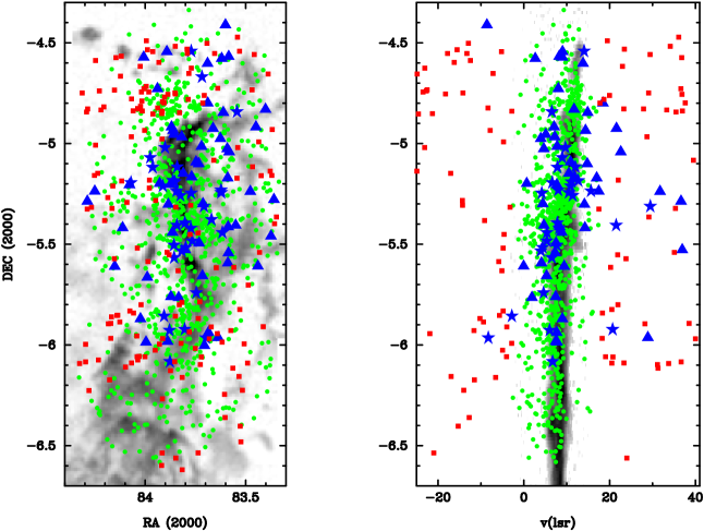
Figure 1: Position and Position-Velocity plot of all targets in the ONC using an average of all velocity measurements. Binaries are plotted with blue symbols those with an IR excess are plotted as star points, without are plotted as triangles, and binaries without photometry are plotted as squares. The red squares represent stars which lie significantly off the cluster velocity, this shows that in general stars with a velocity deviant from the cluster are located in regions without dense gas.

This study continues the monitoring of the targets observed by Fűrész et al. (2008) with the addition of $\sim$200 new targets from the MIKE Fibers observations. The targets are plotted in the left panel of Figure 1 with the ¹³CO map from Bally et al. (1987). The stellar density on the main filament is very high; thus due to limitations of fiber spacing we cannot observe all stars in the densest regions with a single pointing of the MMT. Additional targets were selected as possible members from their NIR colors to fill the remaining fibers in the Hectochelle FOV. The MIKE Fibers fields were positioned in areas of high stellar density to observe the most targets with a single configuration.

2.1 MIKE Fibers Observations

We observed the ONC with MIKE Fibers in January 2007 and March/April 2008 (Table 1). In the first run, only 3 of our 4 fields were observed; during the second run we obtained data for all 4 fields and observed one field twice. Field A is located south of the Orion Nebula, Fields B and C partially overlap and are located on the central ONC, and Field D is located north of the Orion Nebula, on NGC 1977 (Table 1). Due to strong nebular contamination (Paschen continuum emission), many of the spectra in Field B were unusable. Most targets in Fields B, C, and D overlap with targets observed by Hectochelle in Fűrész et al. (2008), Field A observed many new targets not previously observed with Hectochelle due to its location 30^′ south of the Trapezium.

The data were reduced using the Image Reduction and Analysis Facility (IRAF) task ‘ccdproc’, subtracting the overscan, trimming, subtracting the bias and combined our individual exposures with ‘imcombine’ set for cosmic ray rejection. The spectra were extracted using ‘twodspec’, by first tracing the apertures in a quartz flat field frame to create a template of aperture traces to extract the science spectra. Due to weak Thorium-Argon (Th-Ar) lamps (in the early run), the dispersion correction was applied using the the twilight solar spectrum for all fields except C-2 and C-3. The dispersion solution was then corrected for drift during the night by cross-correlating the faint Th-Ar spectra taken with the twilight spectra and the science frames using ’fxcor’. Fields C-2 and C-3 were calibrated using newly installed Th-Ar lamps which produced much better wavelength solutions.

2.2 Hectochelle Observations

In late October 2007, we observed the ONC with Hectochelle. Two epochs of Fields 1 and 2 were observed, and one epoch of field 3 (Table 2). Field 1 was centered on NGC 1977 and Fields 2 and 3 were centered on the central ONC. All the targets in these fields were previously observed by Fűrész et al. (2008). Due to the crowded field, all of the 240 fibers could not be placed on targets; thus, a number of fibers were allocated for sky observations. These apertures were used for subtraction of scattered moonlight and nebular background. In order to subtract the sky observations, it was necessary to normalize the fiber throughputs using the twilight solar spectrum, and then subtract the average spectrum taken from all the sky fibers. The data were reduced using an automated IRAF pipeline developed by G. Furesz which utilizes the standard spectral reduction procedures, similar to our MIKE fibers procedure. A more detailed description of Hectochelle data reduction can be found in Sicilia-Aguilar et al. (2006).

2.3 Radial velocity measurements

To measure the radial velocities of our observed targets, we used the IRAF package ’rvsao’ (Mink & Kurtz, 1998). This package determines the radial velocity of an object by cross-correlating the observed spectrum with a template of known velocity. The quality of the subsequent cross-correlation or signal-to-noise (S/N) is given by R, defined as

$$R=\frac{h}{\sqrt{2}\sigma_{a}}$$ (1)

where $h$ is the height of the peak in the correlation function, and $\sigma_{a}$ is the estimated error from the rms of the antisymmetric portion of the correlation function. The error in the velocity measurement is then dependent on the instrument used and is of the form

$$\sigma_{v}\sim\frac{C}{1+R}$$ (2)

where $C$ is 20 km s^-1 for MIKE Fibers and 14 km s^-1 for Hectochelle based on adding random noise to spectra as in Hartmann et al. (1986).

For the stellar templates, we used libraries of synthetic stellar spectra rather than observed templates. The use of synthetic templates enables us to explore a wider range of stellar parameters than a few observed templates. For the MIKE data, we used the spectral library of Munari et al. (2005); for the Hectochelle, we used the library by Coelho et al. (2005). We used different libraries because the Munari et al. (2005) templates had a resolution of R $\sim$ 20,000 and thus were a better match for the MIKE data; the Coelho et al. (2005) library were R $\sim$ 100,000, and were more appropriate for the higher resolution of Hectochelle. We tested the MIKE data with both the Coelho et al. (2005) and Munari et al. (2005) templates and found that no systematic velocity shift was introduced by using a particular set of templates. In all cases we used a set of templates with surface gravity log(g) = 3.5, effective temperature (T_eff) ranging from 3500 - 7000K in steps of 250K, and Solar metallicity. We found that there was little need to explore a wider parameter space with the templates as the most important factor determining the quality of a correlation was the T_eff of the template.

The velocity and template with the highest R is selected and matched to the appropriate target coordinates and stored in a Starbase database (Roll, 1996). For each target, the coordinates are combined into a truncated 2MASS ID number (2MASSID), throwing out fractional seconds in right ascension and declination. We then used the 2MASSID to match targets with previous observations and photometric catalogs.

For the purposes of comparing the velocity structure of the stars and gas, we have converted our heliocentric radial velocities of each target to the kinematical local standard of rest (LSR) velocities (Kerr & Lynden-Bell, 1986). We only use the LSR velocities in plotting, but give heliocentric radial velocities in our tables.

2.4 Zeropoint Shifts

To compare with the previous Hectochelle studies, it was necessary to correct for zeropoint velocity shifts due to differences in calibration schemes, observations at differing wavelengths (the earlier studies were based on spectra near H$\alpha$), as well as temperature variations within the spectrograph (Sicilia-Aguilar et al., 2006; Fűrész et al., 2006, 2008). There is also a fiber-to-fiber velocity offset within Hectochelle because the calibration lamps do not illuminate the fibers in precisely the same way as astronomical objects. The fiber-to-fiber offsets have been well-characterized and applied to our data; however, these corrections are small compared with overall zeropoint shifts at differing epochs.

We adopted the results of Fűrész et al. (2008) as baseline velocities to shift our observations to match. Though, the observations in Fűrész et al. (2008) were observed in 2 epochs, they ensured that there was enough overlap between epochs to shift all targets to a common zeropoint established by their observations in 2005. Their 2005 epoch was chosen as the zeropoint because those observations were taken with the then new calibration system which is still in use. For Hectochelle, we applied a constant shift for each field given by the mean of a gaussian fit to the distribution of radial velocity differences for each target in a field. The zeropoint shifts for the Hectochelle fields are of order 1 km s^-1, are given in Tables 2. However, many stars in the MIKE Fibers fields were not observed with Hectochelle and few of the overlapping stars had velocity measurements with R $>$ 6. Instead, we shifted the mean velocity, determined by fitting a gaussian, of the stars in a MIKE Fibers field to them mean velocity of stars observed with Hectochelle and within the MIKE Fibers field but not necessarily observed with MIKE Fibers. More simply, we used the cluster velocity to correct the zeropoint rather than individual velocities. The zeropoint variation of the MIKE Fibers (Table 1) fields tend to be larger than those of Hectochelle, likely due to instrumental differences. Though, the shifts for fields A-1 and A-2 are curiously larger than the rest. The error quoted for each zeropoint shift is the uncertainty in the mean of a gaussian fit to the velocity distribution in each field.

2.5 Identifying Spectroscopic Binaries

In addition to precise kinematics, we are able to use the multi-epoch data to identify spectroscopic binaries (SBs) and reduce their effect on the dispersion of stars relative to gas. To identify the SBs, we follow a standard $\chi^{2}$ method (e.g. Hartmann et al., 1986; Maxted et al., 2008) to determine radial velocity variability. For each star, we start by calculating the error-weighted average radial velocity and and standard deviation of the average from the entire set of velocities measured by MIKE Fibers or Hectochelle. We require that the R of a radial velocity measurement be $>$ 6.0 to be used in the average and $\chi^{2}$. We take this somewhat stringent limit of S/N because we do not want to erroneously identify binary stars due to an inaccurate velocity measurement. We also employ this cutoff in R for our kinematic study for the same reasons and it ensures that our velocity errors will be less than the overall cluster velocity dispersion. Each individual measurement error has two components, one is the random error from the cross-correlation (Eq. 2) and the second is error associated with the zeropoint velocity shift listed in Tables 1 & 2. There maybe some additional sources of systematic error which are dependent on the light path through the spectrograph and because this changes with temperature, it is difficult to characterize.

Once we had the average velocity and measurement errors we calculated the reduced $\chi^{2}$

$$\chi^{2}_{r}=\frac{1}{N-1}\sum_{i}^{N}\frac{(RV_{i}-\overline{RV})^{2}}{\sigma_{i}^{2}}.$$ (3)

We then calculated the $\chi^{2}$ probability and counted any stars with P $<$ 0.0001 ($\sim$3.9$\sigma$) as SBs and removed them from the kinematic sample. It is unlikely that we have falsely identified a binary as our total sample size is 1613; however, this assumes that we have accurately determined the associated errors. For those that are not variable, the average radial velocity is then used in our kinematic study. The multi-epoch observations not only enable filtering of binaries but they also yield a more accurate final radial velocity than single measurements alone. Additionally, we detect SBs from the double-peaked appearance of their correlation function. However, we only flag the obvious double-lined binaries (SB2s) which have clear double-peaked correlation functions because quantitative detection by RV variability is more reliable. We have removed certain and potential SB2s from the kinematic sample, but we only include the SBs detected through RV variation and certain SB2s in our analysis of binary properties.

3 Results

We present new velocity measurements for 1124 stars in the ONC with our Hectochelle and MIKE Fibers data combined. In Table 3, we give a summary table of all targets used in this study. We have combined our velocity measurements with those of Fűrész et al. (2008) and give an average velocity for each target. This table also includes targets that we have not re-observed but are still included in the kinematic study. In addition, we include the available optical photometry and have flagged the detected binaries. The rest of the tables give the individual velocity measurements per field for easier identification of observation epoch. Hectochelle fields 1, 2, and 3 are detailed in Tables 4, 5, and 6 respectively and MIKE Fibers fields A, B, C, and D are detailed in Tables 7, 8, 9, and 10 respectively. We include velocities with R $>$ 3.5 in the tables, but in our kinematic study we only use velocities determined with R $>$ 6.0 to ensure the robustness of our results.

3.1 Spectroscopic Binaries

With the addition of these recent observations, we have a built a multi-epoch dataset that can be used to perform an initial characterization of the close binary population in the ONC. The binary population for main sequence solar-type stars has been well determined by Duquennoy & Mayor (1991) and because most stars form in clusters (Lada & Lada, 2003), we would expect the ONC and the main-sequence to have similar binary fractions. Thus far, studies have shown that the fraction of wide binaries ($>$40 AU separation) in the ONC is comparable to the main sequence (Duchêne, 1999) or perhaps slightly deficient (Reipurth et al., 2007). However, (Reipurth et al., 2007) finds that the ONC is certainly deficient in wide binaries compared to regions of isolated star formation (e.g. Taurus, Upper Sco). In contrast to the studies of wide binaries, little work has been done in constraining the binary fraction of the ONC at separations less than 60 AU using radial velocities.

Thus far, we have detected 89 certain spectroscopic binaries from radial velocity variability and double peaks in the correlation function. In addition, we list 48 other stars as possible spectroscopic binaries; they are not included them in our binary analysis but have been removed from the kinematic sample. Of the certain spectroscopic binaries, 74 are identified from radial velocity variability out of 727 stars with multiple observation epochs and 15 are SB2s identified from the double-peaked appearance of their correlation function. Also, 18 of the 74 SBs identified from velocity variability are found to be SB2s. The binaries detected by radial velocity variations are listed in Table 11 and the double-peaked correlation binaries are listed in Table 12. Fűrész et al. (2008) identified 53 stars as spectroscopic binaries from double-peaked correlation functions (27) and velocity variations (26). We do not carry over the possible binary detections of Fűrész et al. (2008) into our study as our data are better suited for binary identification with more epochs and a better region of the optical spectrum. However, we do confirm 4 from velocity variability but none selected by the presence of a double-peaked correlation function. We do not confirm most binaries from velocity variations in because Fűrész et al. (2008) only required R $>$ 4.0 for a reliable velocity; we require R $>$ 6.0. In all, we have multi-epoch velocities for 727 targets: 333 with 2 epochs, 265 with 3, 93 with 4, 22 with 5, 9 with 6 and 5 with 7.

In order to constrain a binary orbit spectroscopically, we must determine 6 parameters: period, angle of ascending node, eccentricity, time of periastron passage, velocity barycenter, and velocity amplitude of primary and secondary. Inclination and angle of the line of nodes cannot be determined by spectroscopic observations alone, and the masses and semi-major axes are related to the velocity amplitudes and eccentricities as outlined in Batten (1973). Furthermore, in most cases the detected binaries are single-lined, meaning we can only determine the orbital elements for the primary and an independent constraint is needed for the masses. Given the number of parameters and epochs we have available, we cannot reasonably constrain the orbital parameters of any binaries in our sample. In fact, cannot claim to have detected even 1 period for most stars. We are also limited by the fact that most binaries with periods longer than 10 days have eccentric orbits and they spend most of their time at low velocities, decreasing detectability.

Given these difficulties, we cannot estimate our completeness with a any degree of certainty; however, we can compare our observed binary fraction to the main-sequence. We have determined the total binary fraction in our sample to be 11.5% and we estimate that we can detect a binary system with a period out to 4000 days. Duquennoy & Mayor (1991) find that $\sim$17.5% of stars have a binary companion with a period less than 4000 days. Thus, our study is at most $\sim$65% complete, but this estimate quite optimistic. At present, this incompleteness is not problem as we are not attempting to constrain the binary frequency of the ONC as of yet. Our goal is to remove the most obvious binaries from kinematic dataset to reduce the dispersion they introduce to our overall measurements of the cluster velocity structure.

Despite the limitations of our binary results, we correlated our target sample with the most recent visual binary study of the ONC by Reipurth et al. (2007). Of the 72 binary stars detected by Reipurth et al. (2007), 44 were observed in our radial velocity study. However, we only identify the stars 0535179-051532 (JW 560) and 0535254-053403 (JW 783) as binaries in our study, the designations in parentheses are from Prosser et al. (1994) and used in Reipurth et al. (2007). The 0535179-051532 system shows both radial velocity variability and a double peaked correlation function. From the correlation function, it even appears that we detect three components in this binary system. The 0535254-053403 system only shows radial velocity variability. We are not surprised that the 42 others were not detected as spectroscopic binaries because many have wide separations and which would not yield detectable velocity variations over our time baseline.

3.2 Kinematic Relation of Stars and Gas

In Figure 1, we plot the spatial distribution of the stars and ¹³CO gas in the left panel and the position-velocity (PV) relationship of the stars and gas in the right panel. We have plotted the detected SBs in Figure 1 as dark blue points, stars for IR excess sources and triangles for non-excess sources; the non-binary stars are plotted as green circles. We clearly see that most of the stars are in close association with the dense filament in the left panel of Fig. 1 and in the right panel we see that most stars have a velocity similar to that of the gas. Additionally, most of the detected SBs have velocities similar to that of the gas, but note that the velocity of SBs that are cluster members with multiple observations will average out to the cluster velocity. Even with many binaries identified, there are still stars that are clearly not following the gas velocity; these are marked as red squares in Fig. 1. One possible reason for these outliers could be undetected binarity. In total, 154 stars have vastly different velocities from the gas and only 63 have multi-epoch coverage; thus many could still potentially be binaries. We will discuss these outliers further in §4.

Looking more closely at the velocity structure of the gas and stars, some features stand out. First, the velocity distributions of the stars in PV space are clearly asymmetric. In Figure 2, we have plotted the velocity histograms of the stars in bins of declination along with a gaussian fit to the distribution, though the distributions are not exactly gaussian. There is a clear tail toward blue-shifted velocities in some bins which is not present toward red-shifted velocities. Then, moving north in declination the peaks of the velocity distribution become red-shifted compared to regions south.

We use the gaussian fits, shown in Figure 2 to estimate the full width at half-maximum (FWHM) of the velocity distribution in a particular bin. The FWHMs of the individual bins for gas and stars, as well as the median R, are listed in Table 13. We have used the median R to estimate the overall error in radial velocity measurement for a bin and then subtracted this error in quadrature from the gaussian sigma; the gaussian fits drawn in Figure 2 are not corrected. After correction, we see that most of the ONC has a velocity FWHM between 3.76 and 7.14 km s^-1. These values compare well to the 1 dimensional FWHM of 5.9 km s^-1 derived by Jones & Walker (1988). We note that FWHM between -5.0 and -5.2^∘ is larger than the rest but, in this range of declination lies the OMC-2 and OMC-3 regions. This range has many stars in its tail toward the blue which is making the gaussian fit overly large. Also, from -5.8^∘ and lower, the velocity dispersion is much smaller than the rest of the measurements. We will discuss the FWHMs further in §4.

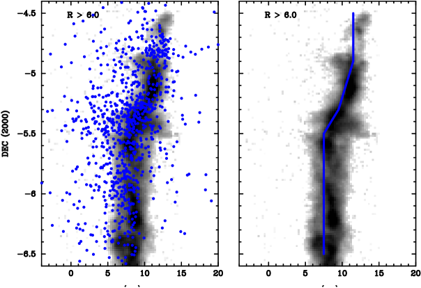
Figure 3: Left: Position-Velocity plot of all non-binary targets, using only Hectochelle data with R $>$ 6.0. Right: Fit to peak of stellar velocity distribution, binned in declination, of the RA range of 84.0 - 83.6^∘. Bins are the same as in Figure 2.

We present a PV plot of a narrow velocity range in the left panel of Figure 3 to more closely show the agreement between the stars and gas. In the right panel of Figure 3, we have plotted a fit to the peak of the velocity distributions shown in Figure 2. However, to fit the peak we have isolated the targets associated with the main filament from 83.6 to 84.0^∘ in RA to minimize outlier contributions. Figure 3 clearly demonstrates that the gas and stars are well correlated within a narrow velocity range over the entire expanse of the molecular cloud. Notably, both the stars and gas show an abrupt shift toward greater velocities at a declination of about -5.4^∘. This velocity shift is reflected in the histogram from -5.2 to -5.4^∘ in Figure 2 as a broad peak in the velocity distribution. The broad peak results from the stellar velocities closely following the molecular gas velocity through the velocity shift. The velocity shift takes place just north of the Trapezium, approximately at the center of the gaseous filament. The characteristic LSR velocity of the gas and stars before the shift is about 8 km s^-1, after the shift it is about 11 km s^-1.

4 Discussion

4.1 Spectroscopic Binary Population

The binary fraction of the ONC has garnered much attention recently. The Hubble Space Telescope has made it possible to observe binary stars in the ONC down to $\sim$0.15^′′ (60 AU) separations. The most recent of these studies find that only $\sim$8.8% of ONC stars are binaries; slightly deficient compared to the field stars and a factor of 2 lower than Taurus (Reipurth et al., 2007). The leading theory for this observation is that dynamical interactions in the dense cluster environment disrupt wide binary systems (Reipurth et al., 2007). In order to test this explanation, we must determine the binary frequency for all separations. This would enable us to tell if all binary systems are deficient or if there is a certain separation distance where the ONC becomes deficient. However, as the visual searches are not sensitive to close separations, a large population of binary stars could still be present but only detectable through radial velocity monitoring.

Presently, we have identified 89 binaries or 11.5% of the total sample with multi-epoch coverage. However, our dataset is not complete enough to yield an accurate final estimate; our value of 11.5% should be regarded as a lower limit. If we used a lower R cutoff for our $\chi^{2}$ routine or lower probability restriction, we would add more binaries to the sample. Further observations will likely confirm additional systems. To characterize the binary systems with respect to the rest of the ONC, we have plotted the detected binaries as crosses on the V - I CMD of the ONC in Figure 4. Most of the binary stars trace a binary sequence with magnitudes slightly greater than the median of the ONC.

Curiously, we have have found that $\sim$30% of our detected binary systems also show an IR excess using the K - IRAC 3.6 $\mu$m versus IRAC 3.6 - 4.5$\mu$m color-color diagram indicating the presence of a circumstellar disk. In Figure 1, the positions of binary stars are plotted, and those having an IR excess are marked with star points. Also, to assess the separation of these systems we plot maximum velocity difference, a surrogate for semi-major axis, versus K - [3.6] in Figure 5. The maximum velocity difference is determined by measuring the difference between correlation peaks for the SB2s and simply the maximum radial velocity minus the minimum for systems detected by velocity variability. We see that some binaries with near-IR excesses at 3.6 $\mu$m also have velocity variations larger than 10 km s^-1, which is $\sim$10AU for a system of 1 M_☉ total mass. The majority of stars with velocity differences $>$ 10 km s^-1 are binaries identified from the double-peaked correlation function.

The significant number of spectroscopic binary systems with near-IR excess is surprising. For most binary systems compact enough to be detected spectroscopically, the companion star is expected to have evacuated the inner disk as in Coku Tau/4 (Ireland & Kraus, 2008). Thus the binaries without a near-IR excess could be transition objects or have an inner disk hole, these objects would then show an IR excess long-ward of 10$\mu$m. Seven others have near-IR excesses but have velocity variations less than 10 km s^-1. These systems may be wider binaries with a truncated outer disk. Perhaps there is an upper limit to the eccentricity of the companion orbit in order to retain the inner disk. This appears to be the case of GG Tau (McCabe et al., 2002) which is shown to have the spectrum of a normal disk (Furlan et al., 2006) and an eccentricity of $\sim$0.3. It is also possible that the disk clearing by the companion has simply not been completed in these relatively young systems. Mid-infrared spectra and MIPS photometry in forthcoming studies from Spitzer and further radial velocity monitoring will constrain the binary orbits and shed light on the disk structure of these young systems.

4.2 Velocity Dispersions

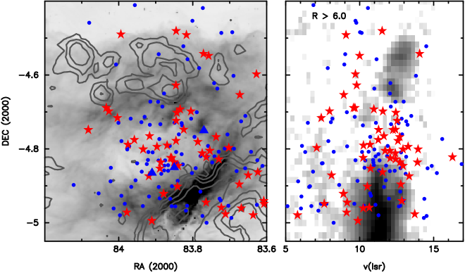
Figure 6: Upper Left: Position plots stars with 5.0 $\geq$ V(LSR) $\geq$ 20.0, the contours are the ¹³CO emission. Upper Right: Position-velocity plot of the region shown in the upper left. Lower Panel: Velocity histogram and gaussian fit for the stars within the RA range of 83.6 - 84.1^∘ and -4.5 - -4.9^∘ in declination. Note that there is no dense gas where we see the densest concentration IR excess stars (stars) and non-excess stars (circles) in the center of the PAH ring. The B stars are marked as large triangles, the most massive star is spectral type B1V at $\alpha$=83.85 $\delta$=-4.85 in the image, this is also the most likely ionization source for the very bright PAH feature directly to its south. The other massive stars are spectra type B3V. Also, the stars within this region have a very tight velocity distribution (lower panel).

In §3, we presented the FWHMs of the ONC binned in declination. We noted that the two most southern and most northern declination bins in Figure 2 have a much lower FWHMs than the rest of the cloud. The FWHM seem to follow the trend of being greater where there is moderately dense gas present, and smaller where there is little gas present or the gas has been evacuated, specifically south of the Orion Nebula and in the NGC 1977 region (Figure 6). The values for the FWHMs of the stars and gas are given in Table 13.

However, looking at the ¹³CO linewidths in Figure 2, we do not observe the trend found in the stellar velocity distributions. Even after correction for measurement error in the radial velocities, most linewidths are more narrow than the stellar velocity distributions by $\sim$2 km s^-1, except in the two most southern regions. Also, there is a trend of larger linewidths south of the Trapezium and smaller linewidths north. The differences between the stellar velocity distribution and the gas line profiles may be due to effects such as unresolved binary motion, gas dispersal, stellar interactions, and/or underestimates of associated errors.

We do notice that not all line profiles are symmetric, though we are making these plots of the ¹³CO by averaging over a large area (0.2^∘ (Dec.)x 0.5^∘ (RA)). Thus in the north the line emission may be dominated by the filament which is kinematically coherent. While in the south, the gas is less dense and there seems to be multiple velocity components in the lines. In the -5.4^∘ to -5.6^∘ bin, there are clearly two velocity components which are probably due to the Trapezium stars blowing the gas away producing a red and blue-shifted component. We can see this structure in more detail in Figure 3, where there is a wide velocity spread in the gas at -5.5^∘ and there is a decrement of intensity compared to regions directly north and south.

4.3 Asymmetry and Outliers in the Velocity Distribution

Thus far, we have discussed how closely the stars follow the gas as shown in Figure 3; however, we clearly see more stars blue-shifted from the gas than are red-shifted. Ordinarily, we would expect there to be an even distribution of blue and red-shifted stars. Some of this asymmetry may be due to a global zeropoint offset between the stellar velocities and the gas velocity. Shown in Figure 2, in some regions the velocity distributions of the stars and gas can differ by about 1 - 1.5 km s^-1. However, a velocity offset between the stars and gas would only account for some of the asymmetry.

There are a few other possibilities that could explain the blue-side asymmetry. One is that the effect could be systematic in nature. Incomplete sky subtraction could cause a slight blue-shift since the heliocentric corrections were always blue-ward of the cluster velocity. Another possibility is that we are detecting a fainter foreground population, though the CMD of stars these slightly blue-shifted stars is not different from the rest of the cluster. In all, we do not know the exact cause of the shift, but its presence does not take away from our results.

In addition to the asymmetry, in the left panel of Figure 1 we see that some stars have velocities more than 10 km s^-1 different from the cluster velocity, 156 in total. We acknowledged in §3 that some of these may be binaries as our multi-epoch coverage is not complete; though, it is unlikely for most of these to be binaries. To examine the spatial relationship of the outliers to the rest of the cluster, the targets with outlying velocities have been plotted as red squares on Figure 1. Many of these deviant velocity targets are located in regions without much ¹³CO emission on the edges of the survey area and there seems to be zone of avoidance around the dense filament. This implies that most of these additional stars selected to fill more fibers are probably foreground sources and not physically associated with the ONC.

We have plotted the sources with V and I-band photometry on the optical CMD in Figure 4 and we have plotted the median V - I color for both the stars within 10 km s^-1 of the gas and those outside 10 km s^-1. We see that the two populations are clearly separated by $\sim$0.2 mag in V - I and $\sim$1 mag V. This separation in the optical CMD suggest and large velocities together strongly suggest that these stars are older and not members of the ONC. The inclusion of stars such as these and binaries in studies of the ONC could be responsible for the wide age spread quoted in some studies (e.g. Jeffries, 2008; Tan et al., 2006). Some of these outlying stars do have IR excesses detected with IRAC photometry; however, we do not have enough observations to confirm that they are not spectroscopic binaries. If these IR excess stars are not binaries, then they may have been dynamically ejected from the ONC, and this would mean that circumstellar disks can survive a strong dynamic interaction. More simply, they could be a members of the older foreground population whose disks have persisted for longer than expected.

4.4 Effects of Stellar Feedback

With all the massive stars in the ONC, we should be able to directly observe its effects on the kinematic structure. As discussed in §4.2, the gas at spatial locations near the Trapezium stars has a very wide spread in velocity as evidenced in Figures 2 & 3, meaning that it is being blown away. However, north of the Trapezium in NGC 1977, we see a region that has been evacuated of dense gas and a ”mini cluster” of stars is left. The most powerful star in NGC 1977 is spectral type B1V (HD 37018) and there are also two B3V stars present (HD 37077 & HD 36958). These stars are fairly weak in comparison to the Trapezium, yet they have nearly evacuated all dense gas within a 1 pc radius. This is a clear demonstration that B-stars rapidly disperse gas; this effect is also seen in the clusters IC348, NGC7129, and IC5146 (Allen et al., 2007, and references therein.). The Spitzer image in the left panel of Figure 6 shows a ring of emission, probably due to Polycyclic Aromatic Hydrocarbons (PAHs), around an evacuated central cluster region (Peterson & Megeath, 2008). This ring was also shown in the MSX images of Kraemer et al. (2003) but not discussed.

Nearly all the stars located inside the PAH ring are located in a very tight velocity group; the stars preferentially occupy the 10 - 15 km s^-1 velocity range, see Figure 6. This group has one of the tightest and most symmetrical velocity distributions in our data. The tight velocity distribution is likely due to the lower mass enclosed by this small cluster due to the evacuation of the gas. The stars with higher velocities probably escaped and may occupy the red and blue-shifted velocity tails in Figure 2. Also, even though most gas is gone, the stars still tightly correlate with the velocity of the gas to the north and south.

There is also some direct evidence for forced ejection of material from this region, in the right panel of Figure 6 there is a faint clump at -4.7^∘ with a blue shifted velocity compared to the stars. Also, in Figure 3, where the PV plot is taken over a wider range in RA, there is a extension of the gas to blue-shifted velocities at -4.85^∘. The gas dispersal must have happened quickly compared to the timescale of disk dissipation as 70% of stars in this regions have an IR excess (Megeath et al. in prep.). Though, because we are bias toward optical stars, only 36% of our surveyed stars have an IR excess.

4.5 Global Kinematic Structure

Our dataset of precise stellar radial velocities, in conjunction with the detailed gas kinematics, provide an unprecedented opportunity to study the dynamics of a cluster whose structure may still reflect the initial conditions of formation. In §3, we roughly outlined how the dense ¹³CO gas and stars occupy the same PV space. The regularity of the velocity structure is quite astounding. In terms of physical sizes, the velocity of the gas and stars correlate well over a 16 pc projected length. However, the northern and southern parts of the cluster have distinctly different characteristic velocities. They are connected by the striking velocity gradient just north of the Orion nebula (OMC-2/3 regions). In a 2 pc (0.25^∘) region, the stars and gas shift toward the red by 2.5 km s^-1. It is important to point out that there is not a corresponding velocity gradient in the southern part of the cluster.

We posit that the velocity gradient in the OMC-2/3 region and distinct kinematics of the north and south regions of the cluster are signatures of large-scale infall. Both the gas and stars seem to be falling in from the north; this is strong evidence that the system is not in dynamical equilibrium. Gravitational collapse presents the simplest explanation for the observed global velocity coherence and why the stars so closely follow the velocity gradient. This condition would of course require that the northern end of the Orion A cloud is somewhat closer than the southern end of the cloud, which is possible given the uncertainties in the 3D structure of the ONC and Orion A cloud. Infall actively taking place in the ONC is very strong evidence for its youth ($\sim$ 1 crossing time, 1 Myr), along with estimated stellar ages (Hillenbrand, 1997).

Our idea of large-scale infall is supported by the N-body simulations of Proszkow et al. (2009). These simulations modeled clusters with parameters similar to the ONC, elongated in the north-south direction and comparable in total mass. They found that a velocity gradient, similar to what is observed in the ONC, could only be present if the the initial conditions of the cluster were sub-virial. If a cluster was initially in virial equilibrium, only a very slight velocity gradient is witnessed. In addition, the magnitude of velocity gradient observed in the model, is highest at the first crossing time. Thus, these simulations, in addition to our kinematic data, are strong evidence that the ONC is a cluster which formed in sub-virial initial conditions and is currently about 1 crossing time in age.

While we argue that sub-virial collapse is the most appealing explanation, several studies have focused on modeling the ONC as a quasi-equilibrium system (e.g. Tan et al., 2006; Scally et al., 2005; Huff & Stahler, 2007). However, the velocity gradient we observe from the north to the south should not be present if the ONC formed in a quasi-equilibrium state. Similarly, we argue that the ONC cannot be much more than 1 crossing time old because if the cloud has been evolving over several dynamical times, the gas will have shocked and the velocity structure should have been washed away. The studies cited above also assume that the stellar population of the central ONC is relaxed. However, it is uncertain if the central ONC is relaxed because the stars just north of the Trapezium follow the velocity gradient. But the there is some evidence for the stars to be undergoing violent relaxation (Feigelson et al., 2005).

Other alternatives could be that a supernova north of the ONC could have induced the shift. However, it is unclear why the velocity of the southern part of the cloud was not shifted as well. Also, large scale rotation of the cloud has been proposed by Kutner et al. (1977) but this possibility does not seem likely because the cloud would be rotating near breakup. Also, stellar feedback could give rise to the velocity gradient, but stellar feedback blows the gas away from the stars. If the velocity gradient was induced a posteriori of star formation, the stars would not should not follow the velocity gradient, which they clearly do.

5 Summary

We have presented new radial velocity measurements for nearly 1124 stars in the ONC, building on the work of Fűrész et al. (2008). With these additional kinematic data, we have refined our determination of the star to gas kinematic relationship in the ONC. The accuracy of the radial velocity measurements has enabled us to clearly show that the stars closely follow the kinematic structure of the moderate density, ¹³CO gas.

We have begun an initial characterization of the spectroscopic binary population of the ONC. We have obtained multi-epoch observations for over half of our total sample and find 89 (11.5%) of the stars to be spectroscopic binaries. However, this number is currently a lower limit at best as we are focusing on detection rather than detailed study of these binaries. We are continuing our radial velocity monitoring program to further identify spectroscopic binary stars in the ONC. In the future, a more directed program is necessary to constrain the orbital parameters of these spectroscopic binaries.

North of the central ONC in NGC 1977, all gas has been evacuated within about $\sim$1 pc of the most luminous star. The stars within this evacuated region occupy a very tight velocity range, possibly indicating that higher velocity stars have escaped after the dispersal of the gas. About 70 % of the stars show an IR excess, thus we can infer that the gas must have been evacuated quickly. This observation shows that even the wimpiest of high mass stars can clear out their surrounding molecular material quickly.

Overall, the most striking feature in the kinematic structure is the sharp velocity shift ($\sim$2.5 km s^-1) toward the red just north of the Trapezium. We argue that this velocity gradient is a signature of large-scale infall; the gas and stars in the OMC-2/3 and NGC 1977 regions have a red-shifted velocity compared to areas farther south and the gradient is traced by both the gas and stars. These observational results taken with the results of recent N-body simulations are consistent with the view of the ONC as a collapsing, sub-virial cluster (Proszkow et al., 2009).

The authors wish to thank the staff of the MMT and Magellan telescopes and the Hectochelle queue observers of Fall 2008 for their efforts in obtaining the data used in this paper. We thank the referee I. Bonnell for helpful comments which helped improve the clarity of this paper. We also thank M. Walker and E. Olszewski for assistance with MIKE Fibers data acquisition/reduction and Jesus Hernandez for useful discussions. J. T. and L. H. acknowledge funding NASA grant 1342979.

Facilities: MMT, Magellan, Spitzer

Figure 2: Velocity histograms and gaussian fits (thin curves) of non-binary stars in the ONC binned in declination. Notice the asymmetry of these distributions and their velocity tail toward lower velocities. Also, as declination increases, the peak of the velocity distribution clearly shifts toward higher, red-shifted velocities. The line profiles of ¹³CO are plotted and are within $\sim$1.5 km/s of the peaks in the stellar distribution. The profiles are generally more narrow that the stellar distributions as velocities with R = 6.0 have $\sim$2 km/s errors.

Figure 4: Optical color magnitude diagrams of our ONC targets with optical photometry from Rebull et al. (2001) and Hillenbrand et al. (1997), the photometry are not corrected for extinction. The left panel is the CMD of stars with radial velocity that is consistent with cluster membership, -2.0 $<$ V(lsr) $<$ 18.0. The right panel is the CMD of stars with velocities outside the velocity range for cluster membership. The dots are stars in our radial velocity catalog and the plus signs overplotted are spectroscopic binaries, we do not separate the binaries based on their average velocity. The solid line in both panels is the median V-I color for stars with velocities consistent with the ONC, the dashed line is the median V-I color for stars with velocities outside the range for cluster membership. The median of the V-I color for both groups of stars show that the stars outside the cluster velocity range are bluer and fainter than the general ONC suggesting that they are indeed a separate population.

Figure 5: Maximum velocity difference from average or difference between correlation peaks for probable binaries versus Ks-band - IRAC 3.6$\mu$m color, a value of K - [3.6] $>$ 0.5 indicates an IR excess. As expected, binary stars without an IR excess are clearly more plentiful than those with excess, though several stars with high velocity differences do have an IR excess which is not expected.

Table 1: MIKE Fibers Observations

Field ID	Start Date	Julian Date	RA	Dec.	Airmass	Exposure Time	Binning	Filter	Zeropoint Shift	Number of Targets
	UT Date	(2454000)	(J2000)	(J2000)		# $\times$ seconds			km s-1
A-1	01-20-2007	120.579	05:35:21.4	-05:57:38.8	1.101	3x1200	2x2	Mg	-5.72 $\pm$ 0.4, 1.98 $\pm$ 0.23	252
B-1	01-21-2007	121.560	05:34:59.7	-05:25:42.2	1.136	3x1200	2x2	Mg	0.54 $\pm$ 0.5	250
C-1	01-24-2007	124.560	05:35:16.40	-05:15:01.4	1.123	3x1200	2x2	Mg	-1.02 $\pm$ 0.4	227
A-2	03-20-2008	555.517	05:35:21.4	-05:57:38.8	1.339	4x1200	2x2	Mg	-4.16$\pm$ 0.38, -3.13$\pm$ 0.23	252
B-2	03-27-2008	552.550	05:34:59.7	-05:25:42.2	1.500	2x1200	2x2	Mg	-1.17 $\pm$ 0.6	250
C-2	03-31-2008	555.515	05:35:16.40	-05:15:01.4	1.279	3x1200	2x2	Mg	-1.17 $\pm$ 0.5	217
C-3	04-03-2008	561.488	05:35:16.40	-05:15:01.4	1.288	3x1200	2x2	Mg	-1.25 $\pm$ 0.5	227
D-2	03-28-2008	553.539	05:35:29.7	-04:50:00.80	1.466	3x1200	2x2	Mg	0.81 $\pm$ 0.6	231

Note. — We only had enough good velocities for Field A to treat the blue and red spectrograph channels independently.

Table 2: Hectochelle Observations

Field ID	Date	Julian Date	RA	Dec.	Airmass	Exposure Time	Binning	Filter	Zeropoint Shift	Number of Targets
	UT Date	(2454000)	(J2000)	(J2000)		# $\times$ seconds			km s-1
F1-E1	10-25-2007	399.000	05:35:13.87	-04:50:15.37	1.317	3x1200	2x2	RV31	0.45 $\pm$ 0.07	192
F1-E2	10-27-2007	400.893	05:35:13.87	-04:50:15.37	1.310	3x1200	2x2	RV31	1.43 $\pm$ 0.04	192
F2-E1	10-27-2007	401.003	05:35:12.75	-05:19:42.90	1.355	3x1200	2x2	RV31	1.40 $\pm$ 0.13	203
F2-E2	10-28-2007	401.836	05:35:12.75	-05:19:42.90	1.602	3x1200	2x2	RV31	1.63 $\pm$ 0.11	203
F3-E1	10-29-2007	402.876	05:35:05.01	-05:26:01.25	1.358	3x1200	2x2	RV31	1.34 $\pm$ 0.24	202

Table 3: Velocity Summary

2massID	RA	Dec.	$\overline{RV}$	N_obs	V	V - I	Multiplicity	Field ID
	(J2000)	(J2000)	(km s-1)
0533179-052138	05:33:17.957	-05:21:38.63	0.0 $\pm$ 0.0	0	18.27	3.29	1	F2-E1, F2-E2, F22
0533204-051123	05:33:20.436	-05:11:23.97	24.3 $\pm$ 0.5	1	17.61	3.09	1	F21
0533225-053240	05:33:22.581	-05:32:40.07	23.9 $\pm$ 1.0	2	16.9	2.51	1	F3-E1, F22
0533233-052153	05:33:23.321	-05:21:53.11	47.2 $\pm$ 0.1	3	16.06	2.03	1	F2-E1, F2-E2, F22
0533234-044234	05:33:23.492	-04:42:34.44	0.0 $\pm$ 0.0	0	0	0	1	F11

Table 4: Hectochelle Field 1 Velocity Data

2massID	RV F1-E1	RV F1-E2	R F1-E1	R F1-E2
	(km s-1)	(km s-1)
0533333-043918	-6.9 $\pm$ 0.2	-6.3 $\pm$ 0.2	41.8	37.1
0533364-044949	21.2 $\pm$ 1.8	27.6 $\pm$ 1.8	9.3	8.5
0533377-043349	26.3 $\pm$ 0.3	25.6 $\pm$ 0.4	28.2	27.4
0533391-043807	27.5 $\pm$ 0.7	29.6 $\pm$ 0.8	10.5	9.3
0533431-044714	25.0 $\pm$ 0.9	25.2 $\pm$ 0.7	9.0	10.6

Table 5: Hectochelle Field 2 Velocity Data

2massID	RV F2-E1	RV F2-E2	R F2-E1	R F2-E2
	(km s-1)	(km s-1)
0533233-052153	47.2 $\pm$ 0.4	47.2 $\pm$ 0.4	20.1	24.1
0533263-051640	67.6 $\pm$ 0.6	49.5 $\pm$ 2.5	12.1	9.4
0533289-050930	106.8 $\pm$ 0.3	106.3 $\pm$ 0.2	31.4	39.6
0533293-050749	32.6 $\pm$ 0.8	31.4 $\pm$ 0.8	11.8	13.3
0533357-050923	30.6 $\pm$ 3.4	31.0 $\pm$ 2.5	9.3	10.6

Table 6: Hectochelle Field 3 Velocity Data

2massID	RV F3-E1	R F1-E1
	(km s-1)
0533225-053240	24.7 $\pm$ 0.9	8.2
0533256-052354	70.3 $\pm$ 0.4	22.8
0533287-052610	30.4 $\pm$ 1.6	5.6
0533298-052735	-17.5 $\pm$ 0.5	18.3
0533301-052257	22.6 $\pm$ 0.6	12.6

Table 7: MIKE Field A Velocity Data

2massID	RV A-1	RV A-2	R A-1	R A-2
	(km s-1)	(km s-1)
0534330-055747	-2.4 $\pm$ 3.6	59.8 $\pm$ 1.9	4.6	9.4
0534338-055638	-7.4 $\pm$ 2.5	-3.8 $\pm$ 1.4	6.9	13.6
0534347-055308	0.0 $\pm$ 0.0	112.3 $\pm$ 4.1	0.0	3.9
0534351-055815	23.0 $\pm$ 2.6	25.1 $\pm$ 2.7	6.9	6.4
0534377-060233	26.4 $\pm$ 1.5	24.1 $\pm$ 1.0	12.4	20.3

Table 8: MIKE Field B Velocity Data

2massID	RV B-1	RV B-2	R B-1	R B-2
	(km s-1)	(km s-1)
0534174-053158	0.0 $\pm$ 0.0	26.2 $\pm$ 4.3	0.0	3.7
0534181-052833	6.3 $\pm$ 4.5	0.0 $\pm$ 0.0	3.5	0.0
0534195-053019	5.1 $\pm$ 4.4	14.0 $\pm$ 3.2	3.5	5.5
0534207-053235	29.1 $\pm$ 3.9	0.0 $\pm$ 0.0	4.2	0.0
0534209-052448	0.0 $\pm$ 0.0	33.8 $\pm$ 3.4	0.0	5.0

Table 9: MIKE Field C Velocity Data

2massID	RV C-1	RV C-2	RV C-3	R C-1	R C-2	R C-3
	(km s-1)	(km s-1)	(km s-1)
0534269-051803	0.0 $\pm$ 0.0	0.0 $\pm$ 0.0	-24.5 $\pm$ 4.4	0.0	0.0	3.6
0534290-051414	25.7 $\pm$ 1.9	20.3 $\pm$ 2.0	21.4 $\pm$ 2.1	9.9	9.1	8.7
0534292-051439	28.2 $\pm$ 1.3	25.3 $\pm$ 1.3	26.3 $\pm$ 1.5	15.2	15.4	13.6
0534302-051148	0.0 $\pm$ 0.0	0.0 $\pm$ 0.0	27.1 $\pm$ 3.1	0.0	0.0	5.5
0534336-051436	25.4 $\pm$ 1.2	24.8 $\pm$ 1.0	26.5 $\pm$ 1.1	15.9	22.8	18.9

Table 10: MIKE Field D Velocity Data

2massID	RV D_1	R D_1
	(km s-1)
0534435-045136	36.9 $\pm$ 3.9	4.2
0534441-044751	10.6 $\pm$ 3.3	5.1
0534452-044758	33.2 $\pm$ 1.9	10.3
0534494-044539	37.9 $\pm$ 1.0	25.4
0534512-044757	35.7 $\pm$ 2.0	9.5

Table 11: Spectroscopic Binaries from Velocity Shifts

RA	Dec.	2massID	$\overline{RV}$	Max. $\Delta$v	log(P)	$\chi^{2}_{r}$	N_obs	V	V - I	K	K - [3.6]	SB	Field ID
(J2000)	(J2000)		(km s-1)	(km s-1)
05:33:26.396	-05:16:40.62	0533263-051640	67.0 $\pm$ 12.7	17.6 $\pm$ 12.8	-44.43	102.31	3	17.95	2.64	12.09	0.15	2	F2-E1, F2-E2, F22
05:33:29.832	-05:27:35.38	0533298-052735	-19.7 $\pm$ 2.7	2.4 $\pm$ 2.8	-4.25	16.24	2	0	0	12.43	0.14	1	F3-E1, F21
05:33:45.47	-05:36:32.40	0533454-053632	18.0 $\pm$ 4.8	3.8 $\pm$ 4.8	-9.20	38.23	2	18.04	3.7	11.00	0.82	1	S1
05:33:47.802	-04:55:03.63	0533478-045503	25.1 $\pm$ 2.5	2.8 $\pm$ 2.6	-7.13	16.41	3	0	0	11.91	0.16	1	F1-E1, F1-E2, F11
05:33:49.54	-05:36:20.52	0533495-053620	24.7 $\pm$ 5.8	6.4 $\pm$ 6.0	-5.80	13.35	3	16.2	2.08	10.71	0.65	1	F2-E1, F2-E2, S3
05:33:54.573	-05:14:15.54	0533545-051415	49.1 $\pm$ 13.9	13.4 $\pm$ 14.0	-64.59	291.31	2	16.93	2.81	10.64	0.22	1	F3-E1, F21
05:34:00.417	-04:36:15.03	0534004-043615	32.4 $\pm$ 8.4	7.3 $\pm$ 9.3	-10.63	24.48	3	0	0	11.80	0.26	2	F1-E1, F1-E2, F11
05:34:07.110	-05:49:25.19	0534071-054925	39.7 $\pm$ 8.1	8.0 $\pm$ 8.3	-6.12	24.46	2	17.25	2.35	12.05	0.15	1	F3-E1, F31
05:34:10.45	-04:50:35.16	0534104-045035	23.8 $\pm$ 2.3	2.8 $\pm$ 2.5	-7.41	12.45	4	13.01	1.2	9.95	0.9	1	F1-E1, F1-E2, S2
05:34:12.029	-05:24:19.63	0534120-052419	22.7 $\pm$ 5.4	3.8 $\pm$ 5.5	-5.13	20.10	2	18.81	3.5	11.57	0.35	1	B-1, B-2, F2-E1, F2-E2, F22
05:34:19.674	-05:02:29.47	0534196-050229	40.4 $\pm$ 5.3	8.6 $\pm$ 5.3	-18.34	29.50	4	17.86	2.82	11.60	0.22	2	F2-E1, F2-E2, F3-E1, F22
05:34:20.315	-04:34:03.43	0534203-043403	26.3 $\pm$ 2.6	2.6 $\pm$ 2.7	-8.49	19.54	3	16.72	2.7	11.57	0.22	1	F1-E1, F1-E2, F11
05:34:22.078	-05:01:34.23	0534220-050134	22.7 $\pm$ 3.9	3.0 $\pm$ 4.0	-5.82	23.15	2	18.45	3.16	12.25	0.54	1	F3-E1, F22
05:34:24.246	-04:24:39.99	0534242-042439	8.8 $\pm$ 3.6	5.0 $\pm$ 3.7	-32.76	75.44	3	0	0	12.48	0	1	F1-E1, F1-E2, F11
05:34:26.741	-04:50:45.60	0534267-045045	32.1 $\pm$ 3.4	3.2 $\pm$ 3.4	-15.36	35.36	3	17.04	2.63	11.33	0.23	1	F1-E1, F1-E2, F11
05:34:28.677	-04:34:39.58	0534286-043439	19.5 $\pm$ 4.6	5.5 $\pm$ 5.8	-4.59	10.57	3	16.4	2.27	11.85	0.14	1	F1-E1, F1-E2, F11
05:34:29.24	-05:14:39.84	0534292-051439	27.8 $\pm$ 2.0	4.2 $\pm$ 2.6	-4.02	4.66	7	15.07	2.27	9.43	0.65	1	C-1, C-2, C-3, F1-E1, F1-E2, S1
05:34:29.50	-05:13:55.20	0534295-051355	26.0 $\pm$ 5.2	5.6 $\pm$ 5.4	-8.06	18.57	3	18.58	2.92	10.43	1.01	1	C-1, C-2, C-3, F2-E1, F2-E2, S2
05:34:32.037	-05:11:24.84	0534320-051124	48.3 $\pm$ 27.0	31.1 $\pm$ 27.0	-163.89	377.37	3	19.95	4.55	11.84	0.37	1	C-1, C-2, C-3, F2-E1, F2-E2, F21
05:34:33.012	-05:57:47.06	0534330-055747	47.0 $\pm$ 19.8	15.1 $\pm$ 19.9	-21.97	96.13	2	16.38	2.37	11.19	0.17	1	A-1, A-2, F31
05:34:37.531	-05:41:17.35	0534375-054117	29.2 $\pm$ 4.2	5.3 $\pm$ 4.4	-6.75	15.53	3	15.92	2.58	10.31	0.24	1	F2-E1, F2-E2, F31
05:34:39.039	-04:55:28.83	0534390-045528	40.4 $\pm$ 12.3	15.7 $\pm$ 12.4	-145.94	226.05	4	17.12	3.02	10.87	0.17	1	F2-E1, F2-E2, F11
05:34:44.447	-05:56:14.87	0534444-055614	25.8 $\pm$ 22.7	22.7 $\pm$ 22.8	-28.38	125.40	2	17.12	2.57	12.24	0.15	1	A-1, A-2, F31
05:34:45.244	-04:47:58.11	0534452-044758	36.3 $\pm$ 6.6	8.2 $\pm$ 6.6	-41.06	94.53	3	17.03	2.55	11.07	0.24	1	D-2, F1-E1, F1-E2, F11
05:34:47.53	-05:57:56.88	0534475-055756	9.9 $\pm$ 31.7	37.4 $\pm$ 31.8	-192.57	297.72	4	14.62	1.67	9.40	0.69	1	A-1, A-2, S3
05:34:49.27	-06:00:11.30	0534492-060011	71.0 $\pm$ 13.9	11.9 $\pm$ 14.1	-9.93	41.50	2	16.35	2.49	11.43	0.29	1	A-1, A-2
05:34:51.754	-05:39:24.12	0534517-053924	23.7 $\pm$ 3.7	3.7 $\pm$ 3.8	-4.28	16.38	2	16.42	2.8	10.78	0.38	1	F3-E1, F21
05:34:52.21	-04:40:11.64	0534522-044011	65.6 $\pm$ 2.7	2.6 $\pm$ 3.2	-20.61	33.03	4	14.38	1.62	9.80	0.73	1	F1-E1, F1-E2, S2
05:34:55.603	-05:29:37.60	0534556-052937	25.5 $\pm$ 6.5	6.0 $\pm$ 6.6	-10.01	41.85	2	18.19	3.26	12.05	0.31	1	B-1, B-2, F2-E1, F2-E2, F21
05:34:56.136	-05:06:01.76	0534561-050601	29.9 $\pm$ 9.6	13.3 $\pm$ 10.3	-4.16	9.57	3	16.87	2.77	11.67	0.27	2	C-1, C-2, C-3, F1-E1, F1-E2, F11
05:34:59.322	-05:05:30.03	0534593-050530	28.8 $\pm$ 2.1	2.7 $\pm$ 2.2	-5.64	12.99	3	16.53	2.45	11.26	0.29	1	C-1, C-2, C-3, F2-E1, F2-E2, F21
05:35:02.096	-05:15:37.46	0535020-051537	28.4 $\pm$ 1.9	2.4 $\pm$ 2.0	-4.11	7.22	4	16.5	2.37	11.79	0.48	1	B-1, B-2, F1-E1, F1-E2, F21
05:35:03.91	-05:29:03.48	0535039-052903	25.6 $\pm$ 15.8	23.2 $\pm$ 15.9	-240.59	371.51	4	14.98	2.25	10.12	0.64	2	B-1, B-2, F2-E1, F2-E2, S3
05:35:04.63	-05:09:55.70	0535046-050955	29.7 $\pm$ 17.5	23.6 $\pm$ 17.6	-30.29	69.75	3	15.73	2.79	10.39	0.18	2	C-1, C-2, C-3
05:35:05.040	-04:32:33.45	0535050-043233	31.9 $\pm$ 6.5	6.8 $\pm$ 6.7	-10.45	24.07	3	17.76	3.08	12.03	0.34	1	F1-E1, F1-E2, F11
05:35:05.21	-05:14:50.28	0535052-051450	20.7 $\pm$ 7.4	9.6 $\pm$ 8.8	-6.96	11.75	4	11.06	1.63	7.19	0.2	1	C-1, C-2, C-3, F1-E1, F1-E2, S1
05:35:05.609	-05:18:24.85	0535056-051824	6.2 $\pm$ 21.4	21.2 $\pm$ 21.5	-34.35	152.71	2	15.53	0	11.25	0.39	1	B-1, B-2, C-1, C-2, C-3, F1-E1, F1-E2, F2-E1, F2-E2, F22
05:35:11.657	-05:31:01.15	0535116-053101	22.1 $\pm$ 6.6	8.7 $\pm$ 6.7	-14.33	33.00	3	18.09	3.25	11.85	0.61	1	B-1, B-2, F3-E1, F21
05:35:12.146	-05:31:38.85	0535121-053138	49.5 $\pm$ 17.9	16.5 $\pm$ 18.0	-66.60	153.36	3	16.95	3.11	11.12	0.22	1	B-1, B-2, F2-E1, F2-E2, F22
05:35:12.33	-05:54:35.20	0535123-055435	25.6 $\pm$ 6.1	4.8 $\pm$ 6.2	-7.05	28.59	2	0	0	13.03	0.35	1	A-1, A-2
05:35:15.953	-05:14:59.04	0535159-051459	27.3 $\pm$ 1.5	1.9 $\pm$ 1.6	-4.71	10.84	3	14.57	1.78	10.32	0.42	1	B-1, B-2, F2-E1, F2-E2, F21
05:35:16.30	-05:32:02.40	0535163-053202	21.4 $\pm$ 8.4	11.2 $\pm$ 8.5	-14.38	33.11	3	18.66	3.61	11.89	0.66	1	B-1, B-2, F3-E1, S3
05:35:17.95	-05:26:50.64	0535179-052650	35.9 $\pm$ 21.4	18.5 $\pm$ 21.5	-39.25	175.14	2	18.72	2.83	11.72	0.83	1	C-1, C-2, C-3, S3
05:35:20.071	-05:45:52.68	0535200-054552	20.0 $\pm$ 22.8	31.2 $\pm$ 23.1	-19.50	44.91	3	0	0	12.14	0.16	1	A-1, A-2, F22
05:35:22.18	-05:24:24.80	0535221-052424	39.4 $\pm$ 28.8	39.0 $\pm$ 28.9	-85.99	197.99	3	13.91	1.89	9.22	0.41	2	C-1, C-2, C-3
05:35:22.63	-05:14:11.04	0535226-051411	35.4 $\pm$ 8.4	12.3 $\pm$ 8.7	-11.95	19.56	4	16.83	3.1	10.29	0.77	2	C-1, C-2, C-3, F3-E1, S3
05:35:24.61	-05:11:29.76	0535246-051129	28.3 $\pm$ 5.0	6.4 $\pm$ 5.2	-8.19	13.68	4	18.9	4	10.39	0.75	1	C-1, C-2, C-3, F2-E1, F2-E2, S1
05:35:26.84	-05:11:07.44	0535268-051107	30.8 $\pm$ 3.0	5.0 $\pm$ 4.2	-9.86	12.99	5	12.26	1.92	7.02	1.22	1	C-1, C-2, C-3, F1-E1, F1-E2, S2
05:35:27.44	-05:26:28.10	0535274-052628	26.7 $\pm$ 4.0	3.9 $\pm$ 4.1	-4.36	10.04	3	14.12	1.75	9.96	0.17	1	C-1, C-2, C-3
05:35:28.167	-05:00:49.57	0535281-050049	42.8 $\pm$ 14.1	13.4 $\pm$ 14.8	-16.83	38.76	3	16.85	2.75	11.54	0.25	1	D-2, F3-E1, F22
05:35:29.896	-05:12:10.39	0535298-051210	60.9 $\pm$ 15.2	25.6 $\pm$ 15.2	-113.85	176.71	4	17.29	2.98	11.74	0.47	2	C-1, C-2, C-3, F1-E1, F1-E2, F3-E1, F21
05:35:30.44	-06:05:00.70	0535304-060500	38.8 $\pm$ 6.1	4.7 $\pm$ 6.3	-6.21	24.85	2	19.68	3.21	13.53	0.6	2	A-1, A-2
05:35:30.930	-05:55:42.34	0535309-055542	24.1 $\pm$ 6.0	7.9 $\pm$ 6.2	-14.34	23.29	4	0	0	12.40	0.51	1	A-1, A-2, F31
05:35:39.923	-04:58:39.27	0535399-045839	-26.5 $\pm$ 57.5	57.4 $\pm$ 57.6	-309.99	1419.84	2	16.8	2.64	11.78	0.2	1	D-2, F11
05:35:42.76	-05:11:54.70	0535427-051154	18.5 $\pm$ 9.8	10.2 $\pm$ 10.1	-7.91	18.22	3	14.01	1.71	10.29	0.11	1	C-1, C-2, C-3
05:35:43.061	-05:03:07.55	0535430-050307	24.9 $\pm$ 4.6	5.7 $\pm$ 4.9	-5.79	9.88	4	18.15	3.06	12.28	0.4	1	F1-E1, F1-E2, F11
05:35:45.096	-04:51:41.84	0535450-045141	20.6 $\pm$ 12.0	10.0 $\pm$ 12.1	-14.12	60.45	2	0	0	12.04	0.28	1	D-2, F1-E1, F1-E2, F11
05:35:45.318	-04:43:39.58	0535453-044339	27.7 $\pm$ 2.8	2.9 $\pm$ 3.3	-12.36	20.20	4	16.58	2.68	10.89	0.18	2	D-2, F1-E1, F1-E2, F11
05:35:50.46	-05:28:35.04	0535504-052835	51.5 $\pm$ 8.2	6.3 $\pm$ 8.3	-9.25	38.46	2	10.3	0.7	6.22	0.6	2	F2-E1, F2-E2, S3
05:35:51.11	-05:07:08.76	0535511-050708	25.7 $\pm$ 1.5	1.9 $\pm$ 1.6	-4.68	8.13	4	14.56	2.14	9.87	0.38	1	C-1, C-2, C-3, F1-E1, F1-E2, S2
05:35:57.519	-05:39:51.39	0535575-053951	63.5 $\pm$ 25.7	35.1 $\pm$ 25.9	-30.79	70.89	3	0	0	11.71	0.19	2	F2-E1, F2-E2, F21
05:35:58.973	-05:59:08.47	0535589-055908	25.9 $\pm$ 4.1	5.1 $\pm$ 4.3	-4.40	10.13	3	16.63	2.34	12.09	0.21	1	A-1, A-2, F31
05:36:16.96	-05:11:42.72	0536169-051142	24.3 $\pm$ 2.3	2.8 $\pm$ 2.4	-7.34	12.34	4	0	0	9.28	0.38	1	F2-E1, F2-E2, S1
05:36:18.788	-05:12:18.25	0536187-051218	25.6 $\pm$ 2.7	3.0 $\pm$ 2.9	-4.80	8.31	4	0	0	12.05	0.2	1	F2-E1, F2-E2, F11
05:36:26.909	-05:25:05.59	0536269-052505	32.8 $\pm$ 11.8	11.2 $\pm$ 11.9	-60.73	273.60	2	17.01	3.1	10.32	0.18	1	F3-E1, F22
05:36:36.335	-05:36:34.11	0536363-053634	27.2 $\pm$ 7.1	9.3 $\pm$ 7.2	-11.55	26.59	3	0	0	11.29	0.14	2	F2-E1, F2-E2, F21
05:37:00.169	-05:14:11.70	0537001-051411	35.9 $\pm$ 4.5	5.5 $\pm$ 4.6	-13.27	30.56	3	0	0	12.11	0.18	1	F2-E1, F2-E2, F21
05:37:09.044	-05:17:12.09	0537090-051712	47.5 $\pm$ 15.8	18.1 $\pm$ 16.5	-16.64	38.32	3	0	0	10.72	0.18	2	F2-E1, F2-E2, F21

Table 12: Spectroscopic Binaries From Cross Correlation

RA	Dec.	2massID	$\overline{RV}$	Est. $\Delta$v	N_obs	V	V - I	K	K - [3.6]	SB	Confidence	Field ID
(J2000)	(J2000)		(km s-1)	(km s-1)
05:33:29.386	-05:07:49.10	0533293-050749	31.4 $\pm$ 3.7	0.0	3	0	0	12.09	0.15	2	2	F2-E1, F2-E2, F22
05:33:35.714	-05:09:23.50	0533357-050923	30.8 $\pm$ 2.2	0.0	3	16.87	2.71	11.41	0.25	2	2	F2-E1, F2-E2, F21
05:33:36.441	-04:49:49.02	0533364-044949	23.8 $\pm$ 3.3	0.0	3	0	0	12.12	0.31	2	2	F1-E1, F1-E2, F11
05:34:21.590	-05:10:13.95	0534215-051013	24.9 $\pm$ 62.5	111.3	3	17.03	2.31	11.86	0.18	2	1	F2-E1, F2-E2, F22
05:34:27.836	-05:43:31.52	0534278-054331	24.1 $\pm$ 2.8	0.0	4	16.89	2.7	11.74	0.18	2	2	F2-E1, F2-E2, F3-E1, F31
05:34:28.52	-05:24:57.96	0534285-052457	24.0 $\pm$ 0.1	0.0	2	13.99	1.63	9.95	0.64	2	2	B-1, B-2, S1
05:34:30.207	-04:58:30.42	0534302-045830	21.9 $\pm$ 2.0	75.8	4	16.32	2.45	11.49	0.18	2	1	F1-E1, F1-E2, F3-E1, F11
05:34:35.681	-05:35:52.09	0534356-053552	25.8 $\pm$ 0.7	0.0	2	17.19	2.47	12.41	0.19	2	2	B-1, B-2, F21
05:34:40.87	-05:22:42.24	0534408-052242	-19.5 $\pm$ 1.1	88.8	1	13.4	1.75	8.60	1.37	2	1	B-1, B-2, F2-E1, F2-E2, S2
05:34:49.98	-05:18:44.64	0534499-051844	57.3 $\pm$ 2.1	0.0	2	10.19	0.9	7.30	1.28	2	2	F2-E1, F2-E2, S1
05:34:52.339	-05:30:08.01	0534523-053008	25.6 $\pm$ 2.5	0.0	1	17.57	3.01	12.13	0.24	2	2	B-1, B-2, F21
05:34:52.763	-05:00:50.91	0534527-050050	24.4 $\pm$ 0.2	22.9	3	17.46	2.86	12.16	0.24	2	1	F1-E1, F1-E2, F11
05:34:53.12	-05:47:42.50	0534531-054742	0.0 $\pm$ 0.0	0.0	0	18.34	2.73	13.16	0.21	2	2	A-1, A-2
05:34:55.63	-06:01:03.60	0534556-060103	14.7 $\pm$ 4.0	0.0	2	15.88	2.14	11.57	0.14	2	2	A-1, A-2
05:34:57.452	-05:30:42.02	0534574-053042	29.8 $\pm$ 2.4	0.0	1	16.54	2.4	11.76	0.2	2	2	B-1, B-2, F21
05:34:59.05	-05:44:29.76	0534590-054429	23.4 $\pm$ 2.4	27.8	4	0	0	10.31	0.8	2	1	F2-E1, F2-E2, S3
05:35:02.497	-05:33:09.95	0535024-053309	26.0 $\pm$ 1.3	0.0	2	15.67	2.3	11.00	0.84	2	2	B-1, B-2, F3-E1, F22
05:35:02.84	-05:51:03.10	0535028-055103	21.6 $\pm$ 2.8	0.0	1	16.34	2.24	11.85	0.15	2	2	A-1, A-2
05:35:03.036	-04:59:59.80	0535030-045959	26.1 $\pm$ 1.5	0.0	3	17.11	2.89	11.72	0.29	2	2	D-2, F2-E1, F2-E2, F21
05:35:04.76	-05:17:42.10	0535047-051742	17.6 $\pm$ 2.5	0.0	1	17.35	3.13	9.34	1.1	2	2	C-1, C-2, C-3
05:35:05.60	-05:25:19.20	0535056-052519	27.3 $\pm$ 1.8	0.0	5	11.52	1.34	7.43	0.74	2	2	B-1, B-2, F2-E1, F2-E2, S1
05:35:06.08	-05:52:39.30	0535060-055239	12.9 $\pm$ 2.7	0.0	1	0	0	11.72	0.16	2	2	A-1, A-2
05:35:06.58	-05:59:51.40	0535065-055951	31.2 $\pm$ 2.4	0.0	1	0	0	12.64	0.25	2	2	A-1, A-2
05:35:06.828	-05:10:38.53	0535068-051038	19.9 $\pm$ 1.1	0.0	1	17.63	3.11	11.60	0.24	2	2	C-1, C-2, C-3, F2-E1, F2-E2, F21
05:35:07.24	-04:50:25.4	0535072-045025	0.0 $\pm$ 0.0	0.0	0	16.8	2.88	11.34	0.23	2	2	D-2
05:35:09.96	-05:57:11.90	0535099-055711	27.0 $\pm$ 5.9	0.0	2	0	0	9.61	1.25	2	2	A-1, A-2
05:35:11.97	-05:20:33.10	0535119-052033	0.0 $\pm$ 0.0	0.0	0	16.85	3.37	8.85	0.66	2	2	C-1, C-2, C-3
05:35:12.59	-05:23:44.16	0535125-052344	25.2 $\pm$ 1.3	28.0	4	12.64	1.62	8.65	0.44	2	1	B-1, B-2, F2-E1, F2-E2, S2
05:35:12.90	-05:59:38.50	0535129-055938	0.0 $\pm$ 0.0	0.0	0	16.36	2.29	11.85	0.13	2	2	A-1, A-2
05:35:14.668	-05:08:52.08	0535146-050852	26.2 $\pm$ 2.2	0.0	4	17.48	3	11.96	0.22	2	2	C-1, C-2, C-3, F1-E1, F1-E2, F2-E1, F2-E2, F11
05:35:15.758	-05:21:39.82	0535157-052139	0.0 $\pm$ 0.0	0.0	0	17.68	2.99	11.38	0	2	2	B-1, B-2, F21
05:35:16.408	-04:58:02.00	0535164-045802	24.2 $\pm$ 0.6	21.5	3	17.73	2.92	12.34	0.28	2	1	D-2, F1-E1, F1-E2, F22
05:35:17.139	-05:12:39.41	0535171-051239	31.7 $\pm$ 6.6	0.0	3	18.74	3.44	12.60	0.3	2	2	C-1, C-2, C-3, F21
05:35:17.92	-05:15:32.76	0535179-051532	28.9 $\pm$ 0.8	29.3	4	17.54	3.37	9.51	0.88	2	1	F1-E1, F1-E2, S1
05:35:18.098	-04:31:19.33	0535180-043119	30.2 $\pm$ 2.6	0.0	3	17.14	2.83	11.79	0.21	2	2	F1-E1, F1-E2, F11
05:35:20.04	-05:21:05.90	0535200-052105	20.3 $\pm$ 1.3	0.0	2	15.09	2.2	8.71	1.09	2	2	C-1, C-2, C-3
05:35:22.817	-05:44:42.89	0535228-054442	42.7 $\pm$ 8.6	0.0	1	0	0	10.64	0.2	2	2	F2-E1, F2-E2, F31
05:35:23.23	-04:43:02.9	0535232-044302	0.0 $\pm$ 0.0	25.7	0	15.08	2.06	10.77	0.09	2	1	D-2
05:35:23.97	-05:59:41.90	0535239-055941	0.0 $\pm$ 0.0	0.0	0	13.77	1.56	10.33	0.11	2	2	A-1, A-2
05:35:24.25	-05:25:18.48	0535242-052518	26.3 $\pm$ 1.6	0.0	1	14.85	1.98	10.04	0.43	2	2	C-1, C-2, C-3, F3-E1, S1
05:35:24.43	-05:24:39.80	0535244-052439	21.6 $\pm$ 2.8	0.0	1	15	2.15	8.91	1.13	2	2	C-1, C-2, C-3
05:35:25.40	-05:51:08.64	0535254-055108	26.9 $\pm$ 0.9	0.0	2	0	0	8.37	1.28	2	2	A-1, A-2, S3
05:35:25.676	-04:57:18.35	0535256-045718	23.9 $\pm$ 4.6	40.0	4	17.92	3	12.37	0.25	2	1	D-2, F1-E1, F1-E2, F11
05:35:26.06	-05:08:37.90	0535260-050837	28.2 $\pm$ 3.4	0.0	3	11.98	1.08	11.57	0	2	2	C-1, C-2, C-3
05:35:26.417	-05:55:26.68	0535264-055526	24.9 $\pm$ 3.8	0.0	3	0	0	12.28	0.52	2	2	A-1, A-2, F31
05:35:26.589	-04:56:06.71	0535265-045606	29.3 $\pm$ 1.3	40.2	4	15.39	2.14	10.93	0.25	2	1	D-2, F1-E1, F1-E2, F2-E1, F2-E2, F22
05:35:28.60	-04:55:03.6	0535286-045503	75.6 $\pm$ 2.8	74.0	1	12.68	1.01	10.29	-0.02	2	1	D-2
05:35:29.307	-05:45:38.17	0535293-054538	26.0 $\pm$ 0.0	24.7	2	0	0	12.02	0.18	2	1	A-1, A-2, F3-E1, F31
05:35:30.48	-05:24:23.00	0535304-052423	0.0 $\pm$ 0.0	0.0	0	14.37	1.89	10.08	0.23	2	2	C-1, C-2, C-3
05:35:30.913	-05:18:17.95	0535309-051817	24.8 $\pm$ 1.1	0.0	3	16.39	3	10.41	0.36	2	2	B-1, B-2, F2-E1, F2-E2, F21
05:35:32.34	-05:18:07.80	0535323-051807	32.0 $\pm$ 5.0	56.8	2	15.88	2.62	10.28	0.18	2	1	C-1, C-2, C-3
05:35:32.52	-05:26:10.40	0535325-052610	0.0 $\pm$ 0.0	0.0	0	15.13	2.11	10.57	0.19	2	2	C-1, C-2, C-3
05:35:33.14	-05:47:07.44	0535331-054707	23.9 $\pm$ 0.7	0.0	2	0	0	12.18	0.32	2	2	A-1, A-2, S3
05:35:33.456	-04:56:01.76	0535334-045601	30.4 $\pm$ 1.9	0.0	2	17.91	3.1	12.06	0.22	2	2	D-2, F1-E1, F1-E2, F22
05:35:33.85	-05:48:21.10	0535338-054821	15.3 $\pm$ 1.5	0.0	2	0	0	12.90	0.23	2	2	A-1, A-2
05:35:34.093	-04:32:37.01	0535340-043237	32.4 $\pm$ 5.5	0.0	3	17.5	2.99	11.91	0.24	2	2	F1-E1, F1-E2, F11
05:35:37.341	-06:00:00.21	0535373-060000	27.2 $\pm$ 0.4	0.0	1	17.26	2.63	12.21	0.24	2	2	A-1, A-2, F31
05:35:37.341	-06:00:00.21	0535373-060000	27.2 $\pm$ 0.4	0.0	1	17.26	2.63	12.21	0.25	2	2	A-1, A-2, F31
05:35:38.214	-05:14:19.02	0535382-051419	29.3 $\pm$ 1.2	0.0	3	16.1	2.86	10.52	0.16	2	2	F2-E1, F2-E2, F21
05:35:39.07	-05:08:56.40	0535390-050856	14.2 $\pm$ 6.5	0.0	2	13.49	1.54	10.00	0.08	2	2	C-1, C-2, C-3
05:35:39.495	-04:40:19.42	0535394-044019	31.1 $\pm$ 1.1	0.0	3	16.8	2.46	11.28	0.14	2	2	D-2, F1-E1, F1-E2, F11
05:35:42.84	-05:51:36.80	0535428-055136	24.8 $\pm$ 2.4	0.0	2	0	0	11.74	0.23	2	2	A-1, A-2
05:35:43.24	-05:09:17.10	0535432-050917	15.4 $\pm$ 7.6	0.0	3	13.79	1.74	9.85	0.09	2	2	C-1, C-2, C-3
05:35:48.853	-05:00:28.56	0535488-050028	25.8 $\pm$ 5.7	0.0	5	17.22	2.57	11.28	0.14	2	2	D-2, F1-E1, F1-E2, F2-E1, F2-E2, F11
05:36:03.355	-04:57:40.48	0536033-045740	23.9 $\pm$ 2.9	0.0	5	17.05	2.51	12.18	0.16	2	2	D-2, F1-E1, F1-E2, F2-E1, F2-E2, F22
05:36:05.655	-05:52:13.08	0536056-055213	27.1 $\pm$ 7.2	23.2	2	0	0	11.97	0.22	2	1	A-1, A-2, F31
05:36:06.601	-05:41:54.38	0536066-054154	27.2 $\pm$ 3.3	0.0	2	0	0	12.61	0.3	2	2	F3-E1, F31

Table 13: Stellar and Gas Full Width Half-Maxima

Dec. of Bin	N	FWHM Stars	Median R	FWHM Stars	FWHM Gas
	Stars	Uncorrected		Corrected
(J2000)		(km s-1)		(km s-1)	(km s-1)
-4.5∘	119	4.97	14.5	4.52	1.48
-4.9∘	120	4.90	15.0	4.45	2.23
-5.1∘	104	7.83	13.2	7.52	1.99
-5.3∘	191	5.54	11.3	4.91	3.20
-5.5∘	146	6.11	13.1	5.66	5.19
-5.7∘	92	6.64	13.4	6.23	3.11
-5.9∘	124	3.43	11.1	2.10	3.04
-6.5∘	157	3.85	15.4	3.24	2.97

References

- Allen et al. (2007) Allen, L., et al. 2007, Protostars and Planets V, 361
- Bernstein et al. (2003) Bernstein, R., Shectman, S. A., Gunnels, S. M., Mochnacki, S., & Athey, A. E. 2003, Proc. SPIE, 4841, 1694
- Bally et al. (1987) Bally, J., Stark, A. A., Wilson, R. W., & Langer, W. D. 1987, ApJ, 312, L45
- Bally et al. (1991) Bally, J., Langer, W. D., Wilson, R. W., Stark, A. A., & Pound, M. W. 1991, Fragmentation of Molecular Clouds and Star Formation, 147, 11
- Ballesteros-Paredes et al. (1999) Ballesteros-Paredes, J., Hartmann, L., & Vázquez-Semadeni, E. 1999, ApJ, 527, 285
- Batten (1973) Batten, A. H. 1973, Binary and multiple systems of stars
- Bonnell et al. (2003) Bonnell, I. A., Bate, M. R., & Vine, S. G. 2003, MNRAS, 343, 413
- Carpenter (2000) Carpenter, J. M. 2000, AJ, 120, 3139
- Coelho et al. (2005) Coelho, P., Barbuy, B., Meléndez, J., Schiavon, R. P., & Castilho, B. V. 2005, A&A, 443, 735
- Duquennoy & Mayor (1991) Duquennoy, A., & Mayor, M. 1991, A&A, 248, 485
- Duchêne (1999) Duchêne, G. 1999, A&A, 341, 547
- Feigelson et al. (2005) Feigelson, E. D., et al. 2005, ApJS, 160, 379
- Fűrész et al. (2006) Fűrész, G., et al. 2006, ApJ, 648, 1090
- Fűrész et al. (2008) Fűrész, G., Hartmann, L. W., Megeath, S. T., Szentgyorgyi, A. H., & Hamden, E. T. 2008, ApJ, 676, 1109
- Furlan et al. (2006) Furlan, E., et al. 2006, ApJS, 165, 568
- Griffin et al. (1988) Griffin, R. F., Griffin, R. E. M., Gunn, J. E., & Zimmerman, B. A. 1988, AJ, 96, 172
- Hartmann et al. (1986) Hartmann, L., Hewett, R., Stahler, S., & Mathieu, R. D. 1986, ApJ, 309, 275
- Hartmann et al. (2001) Hartmann, L., Ballesteros-Paredes, J., & Bergin, E. A. 2001, ApJ, 562, 852
- Hartmann & Burkert (2007) Hartmann, L., & Burkert, A. 2007, ApJ, 654, 988
- Hillenbrand (1997) Hillenbrand, L. A. 1997, AJ, 113, 1733
- Hillenbrand & Hartmann (1998) Hillenbrand, L. A., & Hartmann, L. W. 1998, ApJ, 492, 540
- Huff & Stahler (2007) Huff, E. M., & Stahler, S. W. 2007, ApJ, 666, 281
- Ireland & Kraus (2008) Ireland, M. J., & Kraus, A. L. 2008, ApJ, 678, L59
- Jeffries (2008) Jeffries, R. D. 2008, arXiv:0811.3287
- Jones & Walker (1988) Jones, B. F., & Walker, M. F. 1988, AJ, 95, 1755
- Kerr & Lynden-Bell (1986) Kerr, F. J., & Lynden-Bell, D. 1986, MNRAS, 221, 1023
- Kraemer et al. (2003) Kraemer, K. E., Shipman, R. F., Price, S. D., Mizuno, D. R., Kuchar, T., & Carey, S. J. 2003, AJ, 126, 1423
- Kroupa (2000) Kroupa, P. 2000, New Astronomy, 4, 615
- Kutner et al. (1977) Kutner, M. L., Tucker, K. D., Chin, G., & Thaddeus, P. 1977, ApJ, 215, 521
- Lada & Lada (2003) Lada, C. J., & Lada, E. A. 2003, ARA&A, 41, 57
- Larson (1981) Larson, R. B. 1981, MNRAS, 194, 809
- Mathieu et al. (1986) Mathieu, R. D., Latham, D. W., Griffin, R. F., & Gunn, J. E. 1986, AJ, 92, 1100
- Mathieu (1994) Mathieu, R. D. 1994, ARA&A, 32, 465
- Maxted et al. (2008) Maxted, P. F. L., Jeffries, R. D., Oliveira, J. M., Naylor, T., & Jackson, R. J. 2008, MNRAS, 385, 2210
- McCabe et al. (2002) McCabe, C., Duchêne, G., & Ghez, A. M. 2002, ApJ, 575, 974
- Mink & Kurtz (1998) Mink, D. J., & Kurtz, M. J. 1998, Astronomical Data Analysis Software and Systems VII, 145, 93
- Munari et al. (2005) Munari, U., Sordo, R., Castelli, F., & Zwitter, T. 2005, A&A, 442, 1127
- Peterson & Megeath (2008) Peterson, D. E., & Megeath, T. 2008, arXiv:0809.4006
- Prosser et al. (1994) Prosser, C. F., Stauffer, J. R., Hartmann, L., Soderblom, D. R., Jones, B. F., Werner, M. W., & McCaughrean, M. J. 1994, ApJ, 421, 517
- Proszkow et al. (2009) Proszkow, E., Adams, F. C., Hartmann, L., & Tobin, J. J. 2009, ApJ in press.
- Rebull (2001) Rebull, L. M. 2001, AJ, 121, 1676
- Reipurth et al. (2007) Reipurth, B., Guimarães, M. M., Connelley, M. S., & Bally, J. 2007, AJ, 134, 2272
- Roll (1996) Roll, J. 1996, Astronomical Data Analysis Software and Systems V, 101, 536
- Scally et al. (2005) Scally, A., Clarke, C., & McCaughrean, M. J. 2005, MNRAS, 358, 742
- Shu et al. (1987) Shu, F. H., Adams, F. C., & Lizano, S. 1987, ARA&A, 25, 23
- Sicilia-Aguilar et al. (2006) Sicilia-Aguilar, A., Hartmann, L. W., Fürész, G., Henning, T., Dullemond, C., & Brandner, W. 2006, AJ, 132, 2135
- Szentgyorgyi et al. (1998) Szentgyorgyi, A. H., Cheimets, P., Eng, R., Fabricant, D. G., Geary, J. C., Hartmann, L., Pieri, M. R., & Roll, J. B. 1998, Proc. SPIE, 3355, 242
- Tan et al. (2006) Tan, J. C., Krumholz, M. R., & McKee, C. F. 2006, ApJ, 641, L121
- Tonry & Davis (1979) Tonry, J., & Davis, M. 1979, AJ, 84, 1511
- van Altena et al. (1988) van Altena, W. F., Lee, J. T., Lee, J.-F., Lu, P. K., & Upgren, A. R. 1988, AJ, 95, 1744
- Walker et al. (2007) Walker, M. G., Mateo, M., Olszewski, E. W., Bernstein, R., Sen, B., & Woodroofe, M. 2007, ApJS, 171, 389