We prove that all stationary and spherical symmetric black hole solutions to theories with symmetric target spaces are integrable and we provide an explicit integration method. This exact integration is based on the description of black hole solutions as geodesic curves on the moduli space of the theory when reduced over the time-like direction. These geodesic equations of motion can be rewritten as a specific Lax pair equation for which mathematicians have provided the integration algorithms when the initial conditions are described by a diagonalizable Lax matrix. On the other hand, solutions described by nilpotent Lax matrices, which originate from extremal regular (small) $D=4$ black holes can be obtained as suitable limits of solutions obtained in the diagonalizable case, as we show on the generating geodesic (i.e. most general geodesic modulo global symmetries of the $D=3$ model) corresponding to regular (and small) $D=4$ black holes. As a byproduct of our analysis we give the explicit form of the “Wick rotation” connecting the orbits of BPS and non-BPS solutions in maximally supersymmetric supergravity and its STU truncation.

1 Introduction

The construction and study of black hole solutions in supergravity has a long history. Most of the research on this has focused on extremal black holes, not necessarily preserving supersymmetry (see e.g. [1, 2, 3, 4] for reviews). The preservation of supersymmetry makes an understanding of the string theory microstates easier, while the vanishing of certain supersymmetry variations implies that the second-order equations of motion can be integrated to first-order equations, simplifying the explicit construction of solutions. Recently it has been shown [5, 6, 7, 8, 9] that similar integrations to first-order equations, mimicking the supersymmetry variations, can be carried out for some extremal non-supersymmetric [10, 11, 12] and even some non-extremal solutions [13, 14].

In this note, we will follow a different approach to solve for black hole solutions in supergravity, which does not use (hidden) supersymmetry. We use the fact that the black hole solutions, after performing a dimensional reduction of the supergravity theory over the time direction, are described by geodesic curves on a non-linear sigma model [15], see also [32, 33, 34, 35] for early original work. This idea has recently been fleshed out in more detail to understand the general structure of BPS solutions [16, 17], non-BPS attractors [18], or the general properties of extremal and non-extremal solutions [19]. In case the sigma model is described by a symmetric space $G/H$, the geodesic curves are classified in terms of the Noether charges of the solution. In particular, when the coset representative $\mathbb{L}$ is squared to the symmetric coset matrix, $\mathcal{M}=\mathbb{L}\mathbb{L}^{T}$ , then the solution can be compactly written as [15]

$$\mathcal{M}(t)=\mathcal{M}(0)\,{\rm e}^{Q\,t}\,,$$ (1)

where $Q$ is a matrix containing the Noether charges. This can be seen as a proof of principle that the geodesic equations are integrable. From the knowledge of $Q$ one can extract already a lot of useful information about the black hole solutions [16, 17, 18, 19], but in many cases more is needed to understand the physics of the black hole solutions. For instance, the scalar $U$ describing the black hole geometry is contained in $\mathcal{M}$ and an explicit understanding of the black hole geometry requires the full radial dependence of this scalar. However, extracting the expressions for the scalars out of the expression for $\mathcal{M}$ is a hard problem; hence there is the need for an explicit integration method on the level of the scalars.

The integration procedure we will use has first been introduced in supergravity in constructing time-dependent solutions [20, 21, 22, 23, 24], for which integration through supersymmetry is absent from the very beginning. If the solutions possess Killing directions, they are described by geodesics on a sigma model of a lower-dimensional supergravity, similar to black holes. The difference between time-dependent solutions and stationary solutions is that in the former case the geodesics live in a Riemannian coset, while in the latter case they live in a coset of indefinite signature. This difference matters when constructing solutions and a main characteristic is that the pseudo-Riemannian case is richer and more involved. In the Riemannian case, it was first pointed out in [21] that the geodesic equations could be rewritten as a Lax pair and that an explicit integration procedure had been developed by mathematicians [25]. This was recently used to construct very non-trivial time-dependent solutions in supergravity [24].

One of the main purposes of this paper is to demonstrate that this holds also in the pseudo-Riemannian case. Namely, the geodesic equations can again be written as a Lax pair and the Lax pair is again of a very specific form for which an explicit integration algorithm has been worked out in the mathematical literature [26] assuming that the initial conditions, summarized by giving the Lax matrix at some initial time, are diagonalizable. The latter restriction might seem rather unimportant since non-diagonalizable matrices are a subset of measure zero in the space of matrices. However, ironically, all BPS states (and non-BPS attractive black holes) are described by such initial conditions. It is rather curious that exactly non-extremal solutions are easier to describe than extremal solutions in this Lax pair approach. This demonstrates that the geodesic approach is orthogonal to using (fake) supersymmetry . In this paper we will not yet develop the general Lax integration algorithm for non-diagonalizable initial conditions; we will however already mention that the Lax integration algorithm can be extended to the non-diagonal case. We leave a discussion on this issue for an upcoming paper that will contain more technical details [27]. Here, we simply want to put forward the principle, and illustrate this with simple examples based on the cosets $\mathop{\rm SL}(2,\mathbb{R})/\mathop{\rm SO}(1,1)$ and $\mathop{\rm SL}(3,\mathbb{R})/\mathop{\rm SO}(2,1)$. A second part of our analysis concerns the application to the description of $D=4$ black holes. As we shall show, a class of solutions with non-diagonalizable initial conditions, which can be obtained as limits of solutions with diagonalizable Lax matrices, and which therefore can be derived by our algorithm, are precisely those which are relevant to the description of non-singular (i.e. having no naked singularities) $D=4$ black hole solutions. We shall apply our algorithm to the construction of the generating geodesic of regular (and small) $D=4$ black holes. By generating geodesic we mean the solution to the $D=3$ model which depends on the least number of parameters such that, by applying on it the global symmetries of the model, the most general geodesic can be constructed. Such geodesic unfolds in a simpler submanifold of the scalar manifold containing a characteristic number of $dS_{2}$ factors times ${\rm O}(1,1)$ factors. This solution was originally studied in [19]. Here, we shall further elaborate on it and, as a byproduct, we determine the explicit form of the “Wick rotation” connecting the orbits of BPS and non-BPS solutions in maximally supersymmetric supergravity and its STU truncation.

The outline of the paper is as follows. In section 2 we show that the geodesic equations, that describe black hole solutions in supergravities with symmetric target spaces, can be rewritten in Lax pair form. In section 3 we give a summary of the integration algorithm that allows us to integrate the geodesic equations on pseudo-Riemannian symmetric target spaces in Lax pair form. This algorithm will be illustrated in section 4, using the examples of $\mathop{\rm SL}(2,\mathbb{R})/\mathop{\rm SO}(1,1)$ and $\mathop{\rm SL}(3,\mathbb{R})/\mathop{\rm SO}(2,1)$. In section 5, after recalling some results of [19], we shall make general comments on the solutions corresponding to (non-)diagonalizable initial conditions and show that the generating geodesic with non-diagonalizable initial conditions can be obtained as a limit of solutions with diagonalizable Lax matrices. As an example of solutions with non-diagonalizable initial conditions, the generating geodesic corresponding to extremal $D=4$ regular (and small) black holes will be explicitly constructed in the maximally supersymmetric theory and its STU truncation. Our analysis will show that the Noether charge matrices corresponding to such solutions belong, according to their supersymmetry properties, to different real sections of the same orbit of the complexification of the global symmetry group. Finally, in section 6 we present our conclusions.

In the final stage of preparation of the present paper, we have learned about the interesting paper [28] whose results partially overlap ours.

2 The geodesic equations in Lax pair form

As mentioned in the introduction, in describing cosmological and black hole solutions in supergravity, one often uses the existence of certain Killing vectors in order to reduce the supergravity to a lower dimension. The solutions are then essentially described by geodesics on the non-linear sigma model, spanned by the scalar fields of the lower-dimensional theory [15]. This non-linear sigma model can be either pseudo-Riemannian or Riemannian, depending on whether the reduction to three dimensions includes the time direction or not. In the following, we will consider the case in which the non-linear sigma model is a symmetric space $G/H$, that can be either Riemannian or pseudo-Riemannian. In the former case, $H$ is the maximally compact subgroup of $G$, while in the latter case $H$ is a non-compact subgroup of $G$. In this section, we will show that the geodesic equations for the scalar fields can be rewritten in Lax pair form, establishing their integrability, irrespective of whether $G/H$ is Riemannian or pseudo-Riemannian. The argument proceeds along the same lines as in [21], where $G/H$ was supposed to be Riemannian.

Let $\mathbb{G}$, $\mathbb{H}$ be the Lie algebras of $G$ and of the (not necessarily compact) isotropy group $H$ respectively and let $\mathbb{K}$ be the orthogonal complement of $\mathbb{H}$ in $\mathbb{G}$, as determined by the Cartan decomposition:

$$\mathbb{G}=\mathbb{H}+\mathbb{K}\,.$$ (2)

This decomposition is defined through the use of the Cartan involutive automorphism $\theta$, which acts as

$$\theta(\mathbb{H})=\mathbb{H}\,,\qquad\theta(\mathbb{K})=-\mathbb{K}\,.$$ (3)

Since the automorphism preserves the Lie bracket, we have

$$[\mathbb{H},\mathbb{H}]\subset\mathbb{H}\,,\qquad[\mathbb{H},\mathbb{K}]\subset\mathbb{K}\,,\qquad[\mathbb{K},\mathbb{K}]\subset\mathbb{H}\,.$$ (4)

Let us illustrate this in case $G/H$ is a maximally non-compact coset, i.e. $\mathbb{G}$ is the split real form of a complex Lie algebra $\mathbb{G}_{\mathbb{C}}$. In that case, we have

$$\mathbb{H} =\text{Span}\{t_{\alpha}\}\equiv\text{Span}\{E^{\alpha}+\theta(E^{\alpha})\}\,,$$

$$\mathbb{K} =\text{Span}\{K_{A}\}\equiv\text{Span}\{H_{i},\tfrac{1}{\sqrt{2}}\left(E^{\alpha}-\theta(E^{\alpha})\right)\}\,,$$ (5)

where $H_{i}$ and $E^{\alpha}$ are the Cartan and the positive step operators (i.e. corresponding to positive roots) of the algebra $\mathbb{G}$ respectively. For the cosets that originate from a purely space-like reduction or from a reduction along the time direction, the action of $\theta$ on the step operators is respectively given by [19]:

purely space-like reduction $$:\theta(E^{\alpha})=-E^{-\alpha}\,,$$

reduction including time $$:\theta(E^{\alpha})=-(-1)^{\beta_{0}(\alpha)}E^{-\alpha}$$ (6)

where $\beta_{0}(\alpha)=H_{\beta_{0}}(E^{\alpha})$ represents the grading of the root $\alpha$ with respect to $H_{\beta_{0}}$, the Cartan generator that is associated with the internal time direction. Let us now denote by $\mathbb{L}$ a coset representative. We wish to write the geodesic flow equations in a Lax pair form both in the Riemannian and pseudo-Riemannian cases. We shall generically denote by $t$ the affine parameter along the geodesic, so that the solution will be described by a suitable dependence of the $D=3$ scalar fields on $t$: $\phi^{I}=\phi^{I}(t)$ . The left invariant one-form $\Omega$ on the coset, pulled-back on the geodesic, can be expanded as follows

$$\Omega=\mathbb{L}^{-1}\frac{{\rm d}}{{\rm d}t}\mathbb{L}=\dot{\phi}^{I}\,\mathbb{L}^{-1}\frac{\partial}{\partial\phi^{I}}\mathbb{L}=W^{\alpha}t_{\alpha}+V^{A}K_{A}\equiv W+V\,.$$ (7)

We identify $V$ as the coset vielbein pulled-back to the one-dimensional space parametrized by the affine parameter $t$. The geodesic action reads

$$S=\int{\rm d}t\,\text{Tr}(VV)\propto\int{\rm d}t\,G_{IJ}(\phi)\,\dot{\phi}^{I}\dot{\phi}^{J}\,,$$ (8)

where the trace is defined in some linear representation of $G$ and where we introduced coordinates (scalar fields) on the coset via $V=K_{A}V^{A}_{I}\dot{\phi}^{I}$. To compute the equations of motion we consider a variation of the action (8)

$$\delta S=2\int{\rm d}t\,\text{Tr}[V\delta V]\,.$$ (9)

The variation $\delta V$ can be rewritten by using the following identity

$$\delta\Omega\equiv\delta W+\delta V=[\Omega,\mathbb{L}^{-1}\delta\mathbb{L}]+\frac{{\rm d}}{{\rm d}t}(\mathbb{L}^{-1}\delta\mathbb{L})\,.$$ (10)

The functional $\mathbb{L}^{-1}\delta\mathbb{L}$ can then formally be rewritten using the Cartan decomposition

$$\mathbb{L}^{-1}\delta\mathbb{L}=\delta w+\delta v$$ (11)

where $\delta w$ and $\delta v$ represent the projection of $\mathbb{L}^{-1}\delta\mathbb{L}$ on $\mathbb{H}$, $\mathbb{K}$ respectively. Plugging this in equation (10), and projecting the resulting equation onto the $\mathbb{K}$ subspace (using the commutation relations (4)) we find

$$\delta V=[W,\delta v]+[V,\delta w]+\frac{{\rm d}}{{\rm d}t}\delta v\,.$$ (12)

Finally, upon substituting this expression in the variation of the action and using the cyclicity of the trace, we find

$$\delta S=2\int{\rm d}t\,\text{Tr}\Bigl{[}\bigl{(}[V,W]-\frac{{\rm d}}{{\rm d}t}V\bigr{)}\delta v\Bigr{]}\,,$$ (13)

from which the Lax pair equation follows

$$\frac{{\rm d}}{{\rm d}t}V=[V,W]\,.$$ (14)

In the following, we will always assume that we work with a coset representative $\mathbb{L}$ in solvable gauge. As explained in e.g. [20, 21, 22, 23], this gauge is such that

$$W=V_{>0}-V_{<0}\,,$$ (15)

where $V_{>0(<0)}$ denotes the upper-triangular (resp. lower-triangular) part of $V$ . Note that for pseudo-Riemannian cosets, there is a subtlety in choosing the solvable gauge. This gauge can not in general be chosen globally on the manifold for non-compact $H$. The solvable group defined by the Iwasawa decomposition of $G$ with respect to its maximal compact subgroup describes local patches of the manifold. Only one of these patches is to be considered as physical, namely spanned by the physical fields of the theory. At the boundary of this region some of these fields explode, signalling singularities in the corresponding four dimensional solution. In the physical solvable patch, time-like and null geodesics (originating from regular four dimensional solutions) are complete, while space-like are not, as they reach the boundary at a finite value of the ”proper time”. We will explicitly show this in section 4.1 where we review the simple case in which the scalar manifold $G/H$ is the two-dimensional de Sitter ($dS_{2}$) space-time. This example will be particularly instructive since, as will be shown in Section 5, the generating geodesic (with respect to the action of $G$) of regular black holes in $D=4$ is described as a geodesic in a product of $dS_{2}$ spaces.

Before starting the discussion of the integration algorithm for the Lax pair equation, let us give the expression of the Noether charge matrix in terms of the Lax operator and the coset representative. Using (7) and (14) it is straightforward to show that the following matrix

$$Q = 2\,\mathbb{L}^{-1\,T}\,V^{T}\,\mathbb{L}^{T}\,,$$ (16)

is a constant of motion. It encodes the conserved charges associated with the invariance with respect to the left action of $G$. Let us stress here that $Q$ is an object of $\mathbb{G}$ while $V$, being in $\mathbb{K}$ only transforms under $H$. The action of a global $G$-transformation on $Q$ decomposes into the action of a global $G/H$ transformation on $\mathbb{L}$ whose effect is to move the initial point of the geodesic, and the action of a global $H$-transformation on $V$.

3 The Lax algorithm

In this section, we will consider an algorithm that is useful in solving differential equations that can be written in Lax pair form:

$$\frac{{\rm d}V}{{\rm d}t}=[V,W]\,,$$ (17)

where $V$ and $W$ are $N\times N$-matrices and $W$ is given in terms of $V$ as

$$W=V_{>0}-V_{<0}\,.$$ (18)

For the problem of solving the geodesic equations on symmetric spaces, the Lax operator $V$ is more specifically defined by

$$V(t)=\sum_{A}\mathrm{Tr}\left(\mathbb{L}^{-1}\frac{{\rm d}\mathbb{L}}{{\rm d}t}K_{A}\right)K_{A}\,,$$ (19)

where $K_{A}$ denote the generators of $\mathbb{K}$. As was shown in section 2, with this definition the Lax equation (17) reproduces the geodesic equations on the symmetric space $G/H$, irrespective of whether $G/H$ is Riemannian or pseudo-Riemannian.

Depending on the symmetry properties of the Lax operator $V$, algorithms have been devised that solve the matrix differential equation (17) and lead to an explicit $t$-dependent solution for $V$. After an explicit solution $V_{\mathrm{sol}}(t)$ for the Lax operator $V$ has been found, one can generically solve for the scalars that parametrize the coset manifold, by solving the following system of differential equations:

$$\mathrm{Tr}\left(\mathbb{L}^{-1}\frac{{\rm d}\mathbb{L}}{{\rm d}t}K_{A}\right)=\mathrm{Tr}\left(V_{\mathrm{sol}}(t)K_{A}\right)\,.$$ (20)

As the left-hand-side of these equations depends on the first derivatives of the scalars, this is a system of first-order equations. Depending on the specific parametrization used for the coset representative, one can solve this system in an iterative manner. The main difference between the Riemannian and the pseudo-Riemannian case lies in the symmetry properties of the Lax operator $V$. For Riemannian cosets, one can choose a matrix representation of the Lie algebra, in which all generators $K_{A}$ are symmetric matrices. The Lax operator $V$ is then also given by a symmetric matrix. The algorithm that solves equations (17) was constructed in [25, 29]. For pseudo-Riemannian cosets, the generators $K_{A}$ are in general no longer symmetric. Instead, some of these generators will be symmetric (corresponding to the positive signature directions of the coset), while others will be anti-symmetric matrices (corresponding to the negative signature directions). Also the Lax operator will therefore no longer be a symmetric matrix and will in general be neither symmetric nor anti-symmetric. As was shown in [26], the algorithm of [25, 29] can be extended to include also this case. In the following, we will summarize this extended algorithm. The algorithm for Riemannian spaces can then be found as a special case of the one outlined below.

In [26] an integration algorithm for the Lax equations (17) (with $W$ given by (18)) is outlined, for Lax operators $V$ for which there exists a non-degenerate diagonal matrix $S=\mathrm{diag}(s_{1}\cdots s_{N})$, such that

$$\tilde{V}=VS\qquad\mathrm{is}\ \mathrm{a}\ \mathrm{symmetric}\ \mathrm{matrix}\,.$$ (21)

The fact that this integration algorithm allows us to integrate the geodesic equations for pseudo-Riemannian cosets is then a result of the following theorem:

Theorem 3.1.

For pseudo-Riemannian symmetric spaces, one can always find a suitable space of coset generators $\mathbb{K}$, such that there exists a non-degenerate diagonal matrix $S$ with the property that

$$\forall K_{A}\in\mathbb{K}\quad:\quad K_{A}S=(K_{A}S)^{T}\,.$$ (22)

In order to justify this statement, we note that one can always find a linear representation for which the Cartan involution can be written as

$$\theta(X)=-\eta X^{T}\eta\,,$$ (23)

where $\eta$ is some diagonal matrix that squares to unity. In general, this matrix $\eta$ is given by

$$\eta=\mathrm{diag}(-\mathord{\!\leavevmode\hbox{ \begin{picture}(0.6,0.7)\put(0.0,0.0){\line(1,0){0.5}} \put(0.15,0.0){\line(0,1){0.7}} \put(0.35,0.0){\line(0,1){0.8}} \put(0.3,0.8){\rule{0.5pt}{0.5pt}}\put(0.26,0.78){\rule{0.5pt}{0.5pt}}\put(0.22,0.76){\rule{0.5pt}{0.5pt}}\put(0.18,0.74){\rule{0.5pt}{0.5pt}}\put(0.14,0.72){\rule{0.5pt}{0.5pt}}\put(0.1,0.7){\rule{0.5pt}{0.5pt}}\put(0.06,0.68){\rule{0.5pt}{0.5pt}}\put(0.02,0.66){\rule{0.5pt}{0.5pt}}\put(-0.02,0.64){\rule{0.5pt}{0.5pt}}\put(-0.06,0.62){\rule{0.5pt}{0.5pt}}\put(-0.1,0.6){\rule{0.5pt}{0.5pt}}\put(-0.14,0.58){\rule{0.5pt}{0.5pt}} \end{picture}}}_{p},\mathord{\!\leavevmode\hbox{ \begin{picture}(0.6,0.7)\put(0.0,0.0){\line(1,0){0.5}} \put(0.15,0.0){\line(0,1){0.7}} \put(0.35,0.0){\line(0,1){0.8}} \put(0.3,0.8){\rule{0.5pt}{0.5pt}}\put(0.26,0.78){\rule{0.5pt}{0.5pt}}\put(0.22,0.76){\rule{0.5pt}{0.5pt}}\put(0.18,0.74){\rule{0.5pt}{0.5pt}}\put(0.14,0.72){\rule{0.5pt}{0.5pt}}\put(0.1,0.7){\rule{0.5pt}{0.5pt}}\put(0.06,0.68){\rule{0.5pt}{0.5pt}}\put(0.02,0.66){\rule{0.5pt}{0.5pt}}\put(-0.02,0.64){\rule{0.5pt}{0.5pt}}\put(-0.06,0.62){\rule{0.5pt}{0.5pt}}\put(-0.1,0.6){\rule{0.5pt}{0.5pt}}\put(-0.14,0.58){\rule{0.5pt}{0.5pt}} \end{picture}}}_{q})\,,$$ (24)

for some $p$, $q$. As $\theta(\mathbb{K})=-\mathbb{K}$, we thus find that

$$K_{A}\eta=(K_{A}\eta)^{T}\,,$$ (25)

for $K_{A}\in\mathbb{K}$, implying that one can take $S=\eta$. Note that also Riemannian spaces obey this theorem. Indeed, in that case $S=\mathord{\!\leavevmode\hbox{ \begin{picture}(0.6,0.7)\put(0.0,0.0){\line(1,0){0.5}} \put(0.15,0.0){\line(0,1){0.7}} \put(0.35,0.0){\line(0,1){0.8}} \put(0.3,0.8){\rule{0.5pt}{0.5pt}}\put(0.26,0.78){\rule{0.5pt}{0.5pt}}\put(0.22,0.76){\rule{0.5pt}{0.5pt}}\put(0.18,0.74){\rule{0.5pt}{0.5pt}}\put(0.14,0.72){\rule{0.5pt}{0.5pt}}\put(0.1,0.7){\rule{0.5pt}{0.5pt}}\put(0.06,0.68){\rule{0.5pt}{0.5pt}}\put(0.02,0.66){\rule{0.5pt}{0.5pt}}\put(-0.02,0.64){\rule{0.5pt}{0.5pt}}\put(-0.06,0.62){\rule{0.5pt}{0.5pt}}\put(-0.1,0.6){\rule{0.5pt}{0.5pt}}\put(-0.14,0.58){\rule{0.5pt}{0.5pt}} \end{picture}}}$. The formulas that will be given below can then be easily adapted to the Riemannian case by taking $s_{i}=1$, $\forall i$.

The algorithm itself is an instance of the inverse scattering method and as such constructs the solution $V_{\mathrm{sol}}(t)$ for the Lax operator, starting from the initial conditions contained in the Lax operator $V$ at $t=0$. The first step in establishing the Lax algorithm consists in realizing that the Lax operator can be diagonalized:

$$V\Phi = \Phi\Lambda\,,$$

$$\frac{{\rm d}}{{\rm d}t}\Phi = W\Phi\,,$$ (26)

where $\Lambda=\mathrm{diag}(\lambda_{1},\cdots,\lambda_{N})$ is the diagonal matrix containing the eigenvalues of $V$. The matrix $\Phi$ then contains the eigenvectors of $V$ as its columns. We will denote the eigenvector of $V$ with eigenvalue $\lambda_{k}$ by

$$\phi(\lambda_{k})=\left(\begin{array}[]{c}\phi_{1}(\lambda_{k})\\ \vdots\\ \phi_{N}(\lambda_{k})\end{array}\right)\,.$$ (27)

The matrix $\Phi$ is thus given by

$$\Phi=\left[\phi(\lambda_{1})\cdots\phi(\lambda_{N})\right]=\left[\phi_{i}(\lambda_{j})\right]_{1\leq i,j\leq N}\,.$$ (28)

One can moreover show that $\Phi$ can be chosen such that it obeys the following orthogonality relations:

$$\Phi S^{-1}\Phi^{T}=S^{-1}\,,\qquad\Phi^{T}S\Phi=S\,.$$ (29)

Note that in general $\Lambda$ can be complex. Also $\Phi$ will in general be complex, even if $\Lambda$ is real. Only in the Riemannian case will $\Lambda$ and $\Phi$ be real.

The $t$-dependent solutions for the matrix elements of $\Phi$ are then given by

$$\phi_{i}(\lambda_{k},t)=\frac{{\rm e}^{-\lambda_{k}t}}{\sqrt{D_{i}(t)D_{i-1}(t)}}\left|\begin{array}[]{ccc}s_{1}c_{11}&\cdots&s_{1}c_{1i}\\ \vdots&\ddots&\vdots\\ s_{i-1}c_{i-1,1}&\cdots&s_{i-1}c_{i-1,i}\\ \phi^{0}_{1}(\lambda_{k})&\cdots&\phi^{0}_{i}(\lambda_{k})\end{array}\right|\,.$$ (30)

The quantities $\phi^{0}$ represent the matrix $\Phi$ at $t=0$; i.e. they are obtained from the eigenvalue problem

$$V_{0}\Phi^{0}=\Phi^{0}\Lambda\,,$$

$$\Phi^{0}=\left[\phi^{0}_{i}(\lambda_{j})\right]_{1\leq i,j\leq N}\,,$$ (31)

where $V_{0}=V(0)$. Note that the eigenvalues contained in $\Lambda$ are time-independent, a property often denoted as the iso-spectral property of the Lax operator. The quantities $c_{ij}(t)$ in the formula (30) are given by

$$c_{ij}(t)=\sum_{k=1}^{N}s_{k}^{-1}\,{\rm e}^{-2\lambda_{k}t}\,\phi^{0}_{i}(\lambda_{k})\phi^{0}_{j}(\lambda_{k})\,.$$ (32)

The $D_{k}(t)$ are then given by the determinant of the $k\times k$-matrix with entries $s_{i}c_{ij}(t)$, i.e.:

$$D_{k}(t)=\mathrm{det}\left[\left(s_{i}c_{ij}(t)\right)_{1\leq i,j\leq k}\right]\,.$$ (33)

Note that $s_{i}c_{ij}(0)=\delta_{ij}$ and $D_{k}(0)=1$. Furthermore $D_{0}(t)=1$.

The final solution for the Lax operator is then found as:

$$\left[V_{\mathrm{sol}}(t)\right]_{ij}=s_{j}\sum_{k=1}^{N}s_{k}^{-1}\lambda_{k}\phi_{i}(\lambda_{k},t)\phi_{j}(\lambda_{k},t)\,.$$ (34)

4 Examples

In this section, we will illustrate the previously outlined algorithm using two examples. The choice of the examples is both based on simplicity as well as on physical relevance. The first example deals with the $\mathop{\rm SL}(2,\mathbb{R})/\mathop{\rm SO}(1,1)$ coset, where the geodesics can be found in a closed and rather simple form. We will see that the algorithm indeed leads to the expected results. The second example deals with the $\mathop{\rm SL}(3,\mathbb{R})/\mathop{\rm SO}(2,1)$ coset. Although still simple, this example is also physically relevant, as it can for instance be used to find black hole solutions in four-dimensional Einstein-Maxwell-dilaton theories. This can be done by making use of the $4D$ black holes/ $3D$ $\mathop{\rm SL}(3,\mathbb{R})/\mathop{\rm SO}(2,1)-$geodesics correspondence outlined in the introduction. In this paper, we will restrict ourselves to showing how geodesics on $\mathop{\rm SL}(3,\mathbb{R})/\mathop{\rm SO}(2,1)$ can be produced using the Lax algorithm. The connection between these geodesics and four- dimensional black holes will be worked out more explicitly in a forthcoming paper.

4.1 The $\mathop{\rm SL}(2,\mathbb{R})/\mathop{\rm SO}(1,1)$ example

Let us apply the algorithm to the pseudo-Riemannian coset $\mathop{\rm SL}(2,\mathbb{R})/\mathop{\rm SO}(1,1)$. The Cartan generator $H$ and positive root $E$ are taken to be

$$H=\left(\begin{array}[]{cc}1&0\\ 0&-1\end{array}\right)=\eta\,\,,\,\,\,E=\left(\begin{array}[]{cc}0&1\\ 0&0\end{array}\right)\,.$$ (35)

The Cartan decomposition $\mathbb{G}=\mathbb{H}+\mathbb{K}$ is then determined by

$$\mathbb{H}=\mathrm{Span}\left\{\frac{1}{2}\,(E+E^{T})\right\}\,,\mathbb{K}=\mathrm{Span}\left\{H,\frac{1}{2}\,(E-E^{T})\right\}\,.$$ (36)

This is the two-dimensional de Sitter space-time ($dS_{2}$) which can be represented by the following hyperboloid in $\mathbb{R}^{1,2}$, see Figure 1:

$$-(X^{0})^{2}+(X^{1})^{2}+(X^{2})^{2} = \alpha^{2}\,,$$ (37)

where we shall choose $\alpha^{2}=2$. The physical coordinates (solvable coordinates) $\phi,\,\chi$, related to the four dimensional fields, span half of this space (physical solvable patch) and are related to $X^{\mu}$ as follows: $e^{-\phi}=X^{1}+X^{0}>0,\,e^{-\phi}\,\chi\propto X^{2}$, see Figure 1. These coordinates correspond to choosing the coset representative in the solvable subgroup of ${\rm SL}(2,\mathbb{R})$ defined by the Iwasawa decomposition and will be referred to as the solvable parametrization:

$$\mathbb{L}(\phi,\chi)={\rm e}^{\chi E}{\rm e}^{\frac{\phi}{2}H}\,.$$ (38)

The Lax operator in terms of the scalar fields and their time-derivatives read:

$$V(t) = \frac{1}{2}\,(\mathbb{L}^{-1}\dot{\mathbb{L}}+\eta\,\dot{\mathbb{L}}^{T}\,\mathbb{L}^{-T}\,\eta)=$$ (39)

$$= \frac{1}{2}\,\left(\begin{matrix}\dot{\phi}&e^{-\phi}\,\dot{\chi}\cr-e^{-\phi}\,\dot{\chi}&-\dot{\phi}\end{matrix}\right)\,.$$

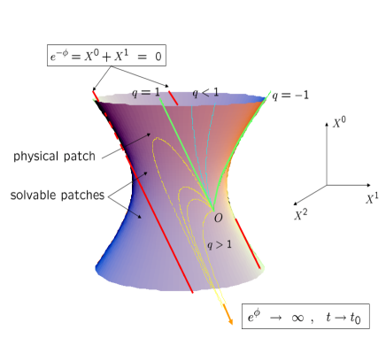
Figure 1: The $dS_{2}$ space-time in $\mathbb{R}^{1,2}$. Some geodesics are represented, for $t<0$. The behavior for $t>0$ is obtained by reflection with respect to the plane containing the $X^{0}$ axis and passing through $O$. Time-like ($|q|<1$) and light-like ($|q|=1$) geodesics are complete, space-like ones are not ($|q|>1$).

Time-like and light-like geodesics, see for instance [15], which arise from regular black holes in four dimensions, are complete in the physical solvable patch. Space-like geodesics on the other hand are not since they cross the boundary $X^{1}+X^{0}=0$ at a finite value of the affine parameter $t$. These solutions however are related to four dimensional black holes with naked singularities. The origin $O$ of the solvable patch, defined by $\phi=\chi=0$, can be mapped into a point $O^{\prime}$ in the other half of the hyperboloid ($X^{1}+X^{0}<0$) by the compact transformation:

$$\mathcal{W} = \exp(\frac{\pi}{2}\,(E-E^{T}))=\left(\begin{matrix}0&1\cr-1&0\end{matrix}\right)\,.$$ (40)

This transformation, being in the coset, does not leave $\eta={\rm}(+1,-1)$ invariant, but instead $\mathcal{W}^{-1}\,\eta\,\mathcal{W}=-\eta$. The lower half of the hyperboloid is still described by solvable coordinates $\phi,\,\chi$, this time parametrizing the coset representative:

$$\mathbb{L}^{\prime}(\phi,\chi)={\rm e}^{\chi E}{\rm e}^{\frac{\phi}{2}H}\,\mathcal{W}\,.$$ (41)

Let us choose the Lax operator at $t=0$ as follows:

$$V_{0}=\left(\begin{array}[]{cc}\frac{a}{\sqrt{2}}&\frac{k}{\sqrt{2}}\\ -\frac{k}{\sqrt{2}}&-\frac{a}{\sqrt{2}}\end{array}\right)=\frac{a}{\sqrt{2}}\,\left(\begin{array}[]{cc}1&-q\\ q&1\end{array}\right)\,,$$ (42)

where $q=-\frac{k}{a}$. This is a diagonalizable initial condition when $|q|\neq 1$. We consider the case where $|q|=1$ separately below. The final solution for the Lax operator $V_{\mathrm{sol}}(t)$ is given by

$$V_{\mathrm{sol}}(t)=\left(\begin{array}[]{cc}V_{11}(t)&V_{12}(t)\\ -V_{12}(t)&-V_{11}(t)\end{array}\right)\,,$$ (43)

where

$$V_{11}(t) =\frac{a^{2}f(t)-f(t)k^{2}-ag(t)\sqrt{a^{2}-k^{2}}}{\sqrt{2}\left(af(t)-g(t)\sqrt{a^{2}-k^{2}}\right)}\,,$$

$$V_{12}(t) =(k\sqrt{a^{2}-k^{2}})/$$

$$\sqrt{2}\Big{(}\text{cosh}\left[\sqrt{2}t\sqrt{a^{2}-k^{2}}\right]\sqrt{a^{2}-k^{2}}$$

$$-a\,\text{sinh}\left[\sqrt{2}t\sqrt{a^{2}-k^{2}}\right]\Big{)},$$ (44)

where we have defined

$$f(t) = -1+{\rm e}^{2\sqrt{2}t\sqrt{a^{2}-k^{2}}}\,,$$

$$g(t) = 1+{\rm e}^{2\sqrt{2}t\sqrt{a^{2}-k^{2}}}\,.$$ (45)

From the above Lax operator, the solutions for the scalar fields can be found. They read, for $|q|<1$ as follows

$$e^{-\phi(t)} = \frac{e^{-\phi_{0}}}{\sqrt{1-q^{2}}}\,\left[\sqrt{1-q^{2}}\,\cosh(x)-\sinh(x)\right]\,,$$ (46)

$$\chi = \chi_{0}+\frac{e^{-\phi_{0}}}{q}-\frac{e^{-\phi_{0}}}{q}\,\left[\frac{1+\frac{q^{2}}{2\,\sqrt{1-q^{2}}}\,\sinh(2\,x)}{1-\frac{q^{2}}{2\,(1-q^{2})}\,(\cosh(2\,x)-1)}\right]\,,$$ (47)

$$x = \sqrt{2\,(1-q^{2})}\,a\,t\,,$$

where $\phi_{0}$ and $\chi_{0}$ are the values of $\phi(t)$ and $\chi(t)$ at $t=0$. These solutions are regular for $x<\frac{1}{2}\,\log\left(\frac{1+\sqrt{1-q^{2}}}{1-\sqrt{1-q^{2}}}\right)$, and thus are complete in the limit $a\,t\rightarrow-\infty$ . For $|q|>1$ the solutions are obtained from the above expressions by writing $x=i\,y=i\,\sqrt{2\,(q^{2}-1)}\,a\,t$:

$$e^{-\phi(t)} = \frac{e^{-\phi_{0}}}{\sqrt{q^{2}-1}}\,\left[\sqrt{q^{2}-1}\,\cos(y)-\sin(y)\right]\,,$$ (48)

$$\chi = \chi_{0}+\frac{e^{-\phi_{0}}}{q}-\frac{e^{-\phi_{0}}}{q}\,\left[\frac{1+\frac{q^{2}}{2\,\sqrt{q^{2}-1}}\,\sin(2\,y)}{1+\frac{q^{2}}{2\,(q^{2}-1)}\,(\cos(2\,y)-1)}\right]\,,$$ (49)

and are regular for $y_{0}<y<y_{1}$ where $y_{1}={\rm Arctan}(\sqrt{q^{2}-1})>0$ and $y_{0}=y_{1}-\pi<0$ are the two points in which $e^{-\phi}$ vanishes. One can explicitly check that the above solutions (46),(47) and (48),(49) do indeed satisfy the geodesic equations. Let us also mention that the norm squared of the geodesic is given by $2\left(a^{2}-k^{2}\right)$. Since the eigenvalues $\lambda_{\pm}$ of $V_{0}$ are given by $\lambda_{\pm}^{2}=\frac{1}{2}\left(a^{2}-k^{2}\right)$, we see that geodesics with real eigenvalues have positive norm squared, while the ones with imaginary eigenvalues correspond to geodesics with negative norm squared.

The behavior of these solutions heavily depends on the values of $a$ and $k$. For instance, upon choosing $a=2$ and $k=1$, one finds that the eigenvalues of the Lax operator are real. The Lax operator is manifestly real and so are the solutions (46),(47) for $\chi$ and $\phi$:

$$e^{-\phi(t)} = \frac{e^{-\phi_{0}}}{\sqrt{3}}\,\left[\sqrt{3}\,\cosh(\sqrt{6}\,t)-2\,\sinh(\sqrt{6}\,t)\right]\,,$$

$$\chi(t) = \chi_{0}+2\,e^{\phi_{0}}-\sqrt{3}\,e^{\phi_{0}}\left[\frac{4\,\sqrt{3}+\sinh(2\,\sqrt{6}\,t)}{7-\cosh(2\,\sqrt{6}\,t)}\right]\,.$$ (50)

In the limits $t\rightarrow\pm\infty$, the Lax operator $V(t)$ reduces to a diagonal matrix. One can also check that, in flowing from $t=-\infty$ to $t=+\infty$, the eigenvalues remain constant. In general, they will however get permuted on the diagonal during the flow.

For $a=1$ and $k=2$ on the other hand, one finds that the Lax operator has purely imaginary eigenvalues $\lambda={\rm i}\sqrt{3/2}$ and $\bar{\lambda}=-{\rm i}\sqrt{3/2}$. The Lax operator itself is still real however. The solutions for $\phi$ and $\chi$ are given by eqs. (48),(49), which read:

$$e^{-\phi(t)} = \frac{1}{\sqrt{3}}\,e^{-\phi_{0}}\,\left[\sqrt{3}\,\cos(\sqrt{6}\,t)-\cos(\sqrt{6}\,t)\right]\,,$$

$$\chi(t) = \chi_{0}+\frac{e^{\phi_{0}}}{2}-\frac{\sqrt{3}}{2}\,e^{\phi_{0}}\,\left[\frac{\sqrt{3}+2\,\sin(2\,\sqrt{6}\,t)}{1+2\,\cos(2\,\sqrt{6}\,t)}\right]\,.$$ (51)

The asymptotics for the Lax operator are now very different from the case in which the eigenvalues are real. The limits $t\rightarrow\pm\infty$ now no longer lead to a diagonal Lax operator. Instead, these limits are not well-defined due to the oscillating character of the functions involved. What is physically relevant is the segment of the curve, of finite length, contained in the physical solvable patch and parametrized by $t\in]t_{0},\,t_{1}[$, corresponding to $y\in]y_{0},\,y_{1}[$, where $t_{0}<0$ and $t_{1}>0$ are the first zeros of $e^{\phi}$ in the neighborhood of the origin $O$.

Note that for the Riemannian case, the Lax operator is a symmetric matrix and the eigenvalues are always real. The Lax operator thus always reduces to a diagonal matrix at $t=\pm\infty$. Indeed, this phenomenon lies at the heart of the cosmic billiard phenomenon (see e.g. [21, 23, 24]).

In case the Lax operator at $t=0$ is non-diagonalizable, namely $|q|=1$, we can have $q=\varepsilon=\pm 1$. The initial value for the Lax operator is:

$$V_{0}=\frac{a}{\sqrt{2}}\,\left(\begin{matrix}1&-\varepsilon\cr\varepsilon&1\end{matrix}\right)=\frac{a}{\sqrt{2}}\,n^{\varepsilon}\,,$$ (52)

where $n^{\varepsilon}$ denotes two nilpotent elements such that, if $J=\frac{1}{2}\,(E+E^{T})=\frac{1}{2}\,\left(\begin{matrix}0&1\cr 1&0\end{matrix}\right)$, we have: $[J,\,n^{\varepsilon}]=\varepsilon\,n^{\varepsilon}$. The solution can be found as the $|q|\rightarrow 1^{-}$ limit of (46),(47) or, equivalently, as the $|q|\rightarrow 1^{+}$ limit of (48),(49) and reads:

$$e^{-\phi(t)} = e^{-\phi_{0}}\,(1-\sqrt{2}\,a\,t)\,,$$ (53)

$$\chi(t) = \chi_{0}-\varepsilon\,e^{\phi_{0}}\,\frac{\sqrt{2}\,a\,t}{1-\sqrt{2}\,a\,t}\,.$$ (54)

This solution is regular as long as $\sqrt{2}\,a\,t<1$. The same solution can be found by directly solving the Lax equation $\dot{V}+[W,V]=0$. Indeed a nilpotent $V(t)$ in the coset can only have the form: $V(t)=\frac{a(t)}{\sqrt{2}}\,n^{\varepsilon}$. In this case we will have: $W=-\varepsilon\,\sqrt{2}\,a(t)\,J$. The Lax equation is then equivalent to $\dot{a}(t)=-\sqrt{2}\,a(t)^{2}$, which is solved by $a(t)=a/(1-\sqrt{2}\,a\,t)$, where we have imposed $a(0)=a$. Substituting in $V(t)$ and using eq. (39) one finds (53) and (54).

This example, analyzed in a certain detail, will be relevant to our discussion of the generating geodesic of regular and small $D=4$ black holes, which will be done in Section 5.

4.2 The $\mathop{\rm SL}(3,\mathbb{R})/\mathop{\rm SO}(2,1)$ example

4.2.1 Solutions for diagonalizable initial conditions

Let us now consider the example of geodesics on $\mathop{\rm SL}(3,\mathbb{R})/\mathop{\rm SO}(2,1)$. We restrict ourselves here to diagonalizable initial conditions. The Cartan generators in the fundamental representation are given by

$$H_{1}=\left(\begin{array}[]{ccc}-\frac{1}{\sqrt{3}}&0&0\\ 0&\frac{2}{\sqrt{3}}&0\\ 0&0&-\frac{1}{\sqrt{3}}\end{array}\right)\,,\qquad H_{2}=\left(\begin{array}[]{ccc}-1&0&0\\ 0&0&0\\ 0&0&1\end{array}\right)\,,$$ (55)

whereas the positive roots are given by

$$E_{12} =\left(\begin{array}[]{ccc}0&1&0\\ 0&0&0\\ 0&0&0\end{array}\right),\qquad E_{23}=\left(\begin{array}[]{ccc}0&0&0\\ 0&0&1\\ 0&0&0\end{array}\right),\qquad$$ (62)

$$E_{13} =\left(\begin{array}[]{ccc}0&0&1\\ 0&0&0\\ 0&0&0\end{array}\right)\,.$$ (66)

The subspaces $\mathbb{H}$ and $\mathbb{K}$ that determine the Cartan decomposition are then explicitly given by

$$\mathbb{H} =\mathrm{Span}\left\{\left(E_{12}+E_{12}^{T}\right),\left(E_{23}+E_{23}^{T}\right),\left(E_{13}-E_{13}^{T}\right)\right\}$$

$$\mathbb{K} =\mathrm{Span}\left\{H_{1},H_{2},\left(E_{12}-E_{12}^{T}\right),\left(E_{23}-E_{23}^{T}\right),\left(E_{13}+E_{13}^{T}\right)\right\}\,.$$

We will define the coset representative as follows

$$\mathbb{L}={\rm e}^{\chi_{1}(t)E_{12}}{\rm e}^{\chi_{0}(t)E_{23}}{\rm e}^{\chi_{2}(t)E_{13}}{\rm e}^{\frac{1}{2}\phi_{1}(t)H_{1}+\frac{1}{2}\phi_{2}(t)H_{2}}\,.$$ (67)

Let us illustrate the behaviour of the solutions with diagonalizable initial conditions by giving two specific examples.

All eigenvalues are real:

The first initial condition we take, is characterized by the following Lax operator at $t=0$:

$$V_{0}=\left(\begin{array}[]{ccc}-1&0&0\\ 0&\frac{1}{2}(1+3\ \text{cosh}[\pi])&-\frac{3\ \text{sinh}[\pi]}{2}\\ 0&\frac{3\ \text{sinh}[\pi]}{2}&\frac{1}{2}(1-3\ \text{cosh}[\pi])\end{array}\right)\,.$$ (68)

The eigenvalues for the Lax operator are all real and given by $-1$, $2$ and $-1$. Running the Lax algorithm, the solutions for the scalars are easily found to be:

$$\phi_{1}(t) = C_{1}+\frac{1}{2}\sqrt{3}(4t-\text{log}[-1+{\rm e}^{6t}(-1+\text{cosh}[\pi])$$

$$- \text{cosh}[\pi]])\,,$$

$$\phi_{2}(t) = C_{2}+\frac{1}{2}\text{log}\left[-1+{\rm e}^{6t}(-1+\text{cosh}[\pi])-\text{cosh}[\pi]\right]\,,$$

$$\chi_{0}(t) = C_{4}+\frac{{\rm e}^{\frac{1}{2}\left(\sqrt{3}C_{1}-C_{2}\right)}\text{coth}\left[\frac{\pi}{2}\right]}{1-{\rm e}^{6t}(-1+\text{cosh}[\pi])+\text{cosh}[\pi]}\,,$$

$$\chi_{1}(t) = C_{3}\,,$$

$$\chi_{2}(t) = C_{5}\,,$$

where $C_{1},\cdots,C_{5}$ are arbitrary integration constants. The behaviour of the Lax operator is very similar to the $\mathop{\rm SL}(2,\mathbb{R})$-example with real eigenvalues. Again, in flowing from $t=-\infty$ to $t=+\infty$ the eigenvalues remain constant and get permuted on the diagonal. This example again corresponds to a geodesic with a positive length squared.

Some eigenvalues are complex:

The second initial condition we take, is characterized by the Lax operator at $t=0$:

$$V_{0}=\left(\begin{array}[]{ccc}-1&0&0\\ 0&1&1\\ 0&-1&0\end{array}\right)\,.$$ (69)

In this case, one eigenvalue is real and given by $-1$, while the other two eigenvalues are complex and given by $\frac{1}{2}\left(1+{\rm i}\sqrt{3}\right)$ and $\frac{1}{2}\left(1-{\rm i}\sqrt{3}\right)$ . Upon applying the Lax algorithm, one finds the following solutions for the scalar fields:

$$\phi_{1}(t) = C_{1}-\frac{1}{2}\sqrt{3}\Big{(}-t+\text{log}\big{[}-3\ \text{cos}\big{[}\sqrt{3}t\big{]}+$$

$$\sqrt{3}\ \text{sin}\big{[}\sqrt{3}t\big{]}\big{]}\Big{)}\,,$$

$$\phi_{2}(t) = C_{2}+\frac{1}{2}\Big{(}3t+\text{log}\big{[}-3\text{cos}\big{[}\sqrt{3}t\big{]}+$$

$$\sqrt{3}\ \text{sin}\big{[}\sqrt{3}t\big{]}\big{]}\Big{)}\,,$$

$$\chi_{0}(t) = C_{4}+\frac{2{\rm e}^{\frac{1}{2}\left(\sqrt{3}C_{1}-C_{2}\right)}\text{sin}\left[\sqrt{3}t\right]}{3\left(-\sqrt{3}\ \text{cos}\left[\sqrt{3}t\right]+\text{sin}\left[\sqrt{3}t\right]\right)}\,,$$

$$\chi_{1}(t) = C_{3}\,,$$

$$\chi_{2}(t) = C_{5}\,,$$

As in the $\mathop{\rm SL}(2,\mathbb{R})$ case with complex eigenvalues, the limits $\lim_{t\rightarrow\pm\infty}V(t)$ are not well-defined and hence do not lead to a diagonal Lax operator, due to the oscillating behaviour of the functions involved in the solutions. In this case, the corresponding geodesic is null-like. A geodesic with negative norm squared can be obtained by applying the Lax algorithm with initial condition

$$V_{0}=\left(\begin{array}[]{ccc}-1&0&0\\ 0&1&2\\ 0&-2&0\end{array}\right)\,,$$ (70)

which again has one real eigenvalue and two complex eigenvalues, that are each others complex conjugates.

4.2.2 Regular solutions for nilpotent initial conditions

After running the Lax algorithm for the initial condition

$$V_{0}=\left(\begin{array}[]{ccc}0&0&1\\ 0&0&a\\ 1&-a&0\end{array}\right)\,,$$ (71)

we obtain the following solutions for the scalars (for $1-a^{2}>0$):

$$\phi_{1}(t)=C_{1}-\frac{1}{2}\sqrt{3}\ \text{log}\left[\text{cosh}\left[2\sqrt{1-a^{2}}t\right]\right]+\frac{\sqrt{3}}{2}\ \text{log}\big{[}$$

$$-a^{2}+\text{cosh}\big{[}2\sqrt{1-a^{2}}t\big{]}\big{]}\,,$$

$$\phi_{2}(t)=C_{2}+\frac{1}{2}\Big{(}\text{log}\big{[}\text{cosh}\big{[}2\sqrt{1-a^{2}}t\big{]}\big{]}+\text{log}\big{[}-a^{2}$$

$$+\text{cosh}\big{[}2\sqrt{1-a^{2}}t\big{]}\big{]}\Big{)}\,,$$

$$\chi_{0}(t)=C_{4}+a\ {\rm e}^{\frac{1}{2}\left(\sqrt{3}C_{1}-C_{2}\right)}\ \text{tanh}\left[2\sqrt{1-a^{2}}t\right]\,,$$

$$\chi_{1}(t)=\frac{{\rm e}^{\frac{1}{2}\big{(}-\sqrt{3}C_{1}-C_{2}\big{)}}}{a^{2}-\text{cosh}\big{[}2\sqrt{1-a^{2}}t\big{]}}\times\Big{(}a+$$

$$a^{2}{\rm e}^{\frac{1}{2}\big{(}\sqrt{3}C_{1}+C_{2}\big{)}}C_{3}-{\rm e}^{\frac{1}{2}\big{(}\sqrt{3}C_{1}+C_{2}\big{)}}C_{3}\ \text{cosh}\big{[}2\sqrt{1-a^{2}}t\big{]}\big{)}\,,$$

$$\chi_{2}(t)=C_{5}+$$

$$\frac{{\rm e}^{-\frac{\sqrt{3}C_{1}}{2}-C_{2}}\left(a\ {\rm e}^{C_{2}/2}\ C_{4}+{\rm e}^{\frac{\sqrt{3}C_{1}}{2}}\text{sinh}\left[2\sqrt{1-a^{2}}t\right]\right)}{-a^{2}+\text{cosh}\left[2\sqrt{1-a^{2}}t\right]}\,.$$ (72)

In the limit $a\rightarrow 1$, the initial condition (71) becomes nilpotent and the solutions (4.2.2) become singular. One can however renormalize the constants $C_{1}$ and $C_{2}$ in such a way that the renormalized solutions are regular in the limit $a\rightarrow 1$ and are still valid solutions of the geodesic equations in this limit.

How this renormalization should be performed can be easily seen by looking at the series expansion of the solutions around $a=1$. For $\phi_{1}(t)$ and $\phi_{2}(t)$, we get

$$\phi_{1}(t) = \left(C_{1}+\frac{\sqrt{3}}{2}\text{log}[-1+a]+\frac{\sqrt{3}}{2}\text{log}\left[-2-4t^{2}\right]\right)+$$ (73)

$$\frac{\sqrt{3}\left(3+30t^{2}+40t^{4}\right)(a-1)}{12+24t^{2}}+O[a-1]^{3/2},$$

$$\phi_{2}(t) = \Big{(}C_{2}+\frac{1}{2}\text{log}[-1+a]+\frac{1}{2}\text{log}\big{[}-2-4t^{2}\big{]}\Big{)}+$$

$$\frac{\big{(}3-18t^{2}-56t^{4}\big{)}(a-1)}{12\big{(}1+2t^{2}\big{)}}+O[a-1]^{3/2}\,.$$

(Let us ignore for the moment the fact that some terms seem complex instead of real. We shall deal with that later.) In both cases, the infinity in taking the limit $a\rightarrow 1$ comes from the second term in the expansion, while all other terms are completely regular.

The solutions for $\phi_{1}(t)$ and $\phi_{2}(t)$ can thus be made regular in this limit, by renormalizing (redefining) $C_{1}$ and $C_{2}$ as

$$C_{1} \rightarrow \frac{1}{2}\sqrt{3}\ \text{log}\left[-\frac{p_{1}}{-1+a}\right]\,,$$

$$C_{2} \rightarrow \frac{1}{2}\ \text{log}\left[-\frac{p_{2}}{-1+a}\right]\,.$$ (74)

Note that we will take the new integration constants $p_{1}$ and $p_{2}$ to be positive. From the series expansion above, it is then immediate that the solutions for $\phi_{1}(t)$ and $\phi_{2}(t)$ become regular in the limit $a\rightarrow 1$:

$$\phi_{1}(t) = \frac{1}{2}\sqrt{3}\left(\text{log}\left[p_{1}(2+4t^{2})\right]\right)\,,$$

$$\phi_{2}(t) = \frac{1}{2}\left(\text{log}\left[p_{2}(2+4t^{2})\right]\right)\,.$$ (75)

It’s an amusing fact that the constants $C_{1}$ and $C_{2}$ appear in the solutions for $\chi_{0}(t)$, $\chi_{1}(t)$ and $\chi_{2}(t)$ in such a way as to render them regular as well in the limit $a\rightarrow 1$ after performing the renormalization:

$$\chi_{0}(t) = \frac{-2\sqrt{2}\ (p_{1}p_{2})^{3/4}t}{p_{2}}+C_{4}\,,$$

$$\chi_{1}(t) = -\frac{1}{2\left(p_{1}^{3}p_{2}\right)^{1/4}\left(1+2t^{2}\right)}+C_{3}\,,$$

$$\chi_{2}(t) = -\frac{2\sqrt{2}p_{1}\sqrt{p_{2}}t-\left(p_{1}p_{2}^{3}\right)^{1/4}C_{4}}{2p_{1}p_{2}+4\text{p1}p_{2}t^{2}}+C_{5}\,.$$ (76)

Note that the above solutions are real for $p_{1},p_{2}>0$. One can also check that they obey the geodesic equations.

5 Relation to the black hole generating geodesic

As already emphasized, the algorithm discussed in the present note is well defined only for solutions corresponding to diagonalizable initial conditions. Although these solutions may yield, in certain limits, geodesics with non-diagonalizable initial data, it is not proven that the most general solution of the latter type can be obtained in this way. However the generating geodesic of regular $D=4$ black holes (including those with vanishing horizon area, i.e. small black holes), defined as the simplest solution capturing all the $G$-invariant properties of the most general one, can be obtained as a singular limit of solutions with diagonalizable $Q$. This generating geodesic was described in [19] as a geodesic within a simple characteristic submanifold of $G/H$ consisting of a product of $dS_{2}$ spaces times $\mathbb{R}_{+}$ factors. This analysis also applies to extremal solutions, since one can show that the Noether charge matrices of light-like geodesics in this simple submanifold have representatives in all the nilpotent orbits corresponding to the regular extremal $D=4$ solutions (including small black holes). Let us first recall the construction made in [19] of the generating geodesic of regular $D=4$ black holes. Then we shall further elaborate on it and work out the explicit transformation mapping the BPS and non-BPS extremal solutions. This transformation belongs to the complexification $G^{\mathbb{C}}$ of $G$ but not to $G$ and its action on the generating geodesics is quite easy to characterize, having the latter very simple form. For the sake of simplicity we shall restrict our analysis to the maximally supersymmetric supergravity and to the $\mathcal{N}=2$ STU model.

We need to first briefly recall the relation between $D=4$ static, single center, asymptotically flat black holes and geodesics on $G/H$. Let us start from a $D=4$ extended supergravity with a symmetric scalar manifold of the form $G_{4}/H_{4}$, spanned by $n_{S}$ scalars $\phi^{r}$ and describing $n_{V}$ vector fields $A^{\Lambda}_{\mu}$. Being $G_{4}/H_{4}$ Riemannian, it is globally described by the solvable group $\mathcal{S}_{4}=\exp(Solv_{4})$ defined by the Iwasawa decomposition of $G_{4}$ with respect to $H_{4}$ and parametrized by $\phi^{r}$: $Solv_{4}=\{\phi^{r}s_{r}\}$. The ansatze for the four dimensional metric and the symplectic vector $\mathbb{F}^{M}_{\mu\nu}$ consisting of the electric field strengths $F^{\Lambda}_{\mu\nu}$ and their magnetic duals $G_{\Lambda\,\mu\nu}\propto\,{}^{\star}\delta\mathcal{L}_{4}/\delta F^{\Lambda}$ read:

$${\rm d}s^{2} = -e^{2\,U}\,{\rm d}t^{2}+e^{-2\,U}\,\left[\frac{c^{4}}{\sinh^{4}(c\,\tau)}\,{\rm d}\tau^{2}+\frac{c^{2}}{\sinh^{2}(c\,\tau)}\,({\rm d}\theta^{2}+\sin(\theta)\,{\rm d}\varphi^{2})\right]\,,$$

$$\mathbb{F} = \left(\begin{matrix}F^{\Lambda}_{\mu\nu}\cr G_{\Lambda\,\mu\nu}\end{matrix}\right)\,\frac{dx^{\mu}\wedge dx^{\nu}}{2}=-e^{2\,U}\mathbb{C}\cdot\mathcal{M}_{4}(\phi^{r})\cdot\Gamma\,{\rm d}t\wedge{\rm d}\tau+\Gamma\,\sin(\theta)\,{\rm d}\theta\wedge{\rm d}\varphi\,,$$ (77)

where $c$ is the extremality parameter, $\mathbb{C}^{MN}$ denotes the $2\,n_{V}\times 2\,n_{V}$ symplectic invariant matrix, $\mathcal{M}_{4}(\phi^{r})\equiv-\mathbb{L}_{4}\,\mathbb{L}_{4}^{T}<0$, $\mathbb{L}_{4}\in\mathcal{S}_{4}$ being the $G_{4}/H_{4}$ coset representative in the symplectic $2\,n_{V}$-dimensional representation, and $\Gamma^{M}\equiv(p^{\Lambda},\,q_{\Lambda})$ the quantized magnetic and electric charges. Let us stress that in the present section the radial variable $\tau$ plays the role of the variable $t$ of the previous sections, not to be confused with the time coordinate $t$. The global symmetry group of the $D=4$ theory is $G_{4}$ which acts simultaneously as an isometry on $\phi^{r}$ and by means of linear symplectic electric-magnetic transformations on $\mathbb{F}^{M}$. The charge vector $\Gamma^{M}$ therefore transform in a symplectic representation ${\bf R}$ of $G_{4}$. The radial variable $\tau$ is by definition negative. The horizon is located at $\tau\rightarrow-\infty$ while radial infinity corresponds to $\tau\rightarrow 0^{-}$.

Upon reduction along the time direction to $D=3$ and dualization of the $D=3$ vector fields into scalars, we end up with $D=3$ gravity coupled to a sigma model whose $2+2\,n_{V}+n_{S}$ scalars $\phi^{I}$ consist in $U$ and the dual $a$ to the Kaluza-Klein vector, coming from the metric, the $D=4$ scalars $\phi^{r}$ and $2\,n_{V}$ scalar fields $\mathcal{Z}^{M}=(\zeta^{\Lambda},\,\tilde{\zeta}_{\Lambda})$ originating from the vector fields and satisfying the relation: $\frac{{\rm d}}{{\rm d}\tau}\mathcal{Z}^{M}=\mathbb{F}^{M}_{0\tau}$. The sigma model metric reads:

$${\rm d}{\bf s}^{2} = G_{IJ}\,{\rm d}\phi^{I}\,{\rm d}\phi^{J}=2\,({\rm d}U)^{2}+G_{rs}\,{\rm d}\phi^{r}\,{\rm d}\phi^{s}+\frac{1}{2}\,e^{-4\,U}\,\omega^{2}+e^{-2\,U}\,{\rm d}\mathcal{Z}^{T}\cdot\mathcal{M}_{4}\cdot{\rm d}\mathcal{Z}\,,$$ (78)

where $\omega\equiv{\rm d}a+\mathcal{Z}^{T}\,\mathbb{C}\,d\mathcal{Z}$. The signature of $G_{IJ}$ clearly has $2\,n_{V}$ minus signs corresponding to the $d\mathcal{Z}$ directions. The global symmetry group $G$ of the $D=3$ Euclidean theory contains the product $\mathop{\rm SL}(2,\mathbb{R})_{E}\times G_{4}$, where $\mathop{\rm SL}(2,\mathbb{R})_{E}$, generated by $\mathfrak{sl}(2,\mathbb{R})_{E}\equiv{\rm Span}(H_{\beta_{0}},\,E_{\beta_{0}},\,E_{-\beta_{0}}$), see footnote 4, is the Ehlers group acting transitively on $U,\,a$. Similarly $H$ contains $\mathrm{U}(1)_{E}\times H_{4}$, where $\mathrm{U}(1)_{E}$ is the compact subgroup of $\mathop{\rm SL}(2,\mathbb{R})_{E}$, generated by $E_{\beta_{0}}-E_{-\beta_{0}}$. The charge vector $\Gamma^{M}$ transforms in a symplectic representation of $\mathrm{U}(1)_{E}\times H_{4}$ which we shall still denote, with an abuse of notation, by ${\bf R}$. The solvable group which describes the physical patch of $G/H$ is defined by the Iwasawa decomposition of $G$ with respect to its maximal compact subgroup (i.e. the compact form of the complexification of $H$) and its generating solvable Lie algebra $Solv={\rm Span}(s_{I})$ is parametrized by $\phi^{I}$. The algebra $Solv$ decomposes with respect to $Solv_{4}$, parametrized by $\phi^{r}$, as follows:

$$Solv = {\rm Span}(H_{\beta_{0}},\,E_{\beta_{0}})\oplus Solv_{4}\oplus{\bf R}_{+1}\,,$$ (79)

where the space ${\bf R}_{+1}\equiv{\rm Span}(s_{M})$ is parametrized by the scalars $\mathcal{Z}^{M}$ and the grading refers to $H_{\beta_{0}}$. Together with the grading $+2$ generator $E_{\beta_{0}}$, the nilpotent generators $s_{M}$ close a Heisenberg algebra: $[s_{M},\,s_{N}]=\frac{1}{2}\,\mathbb{C}_{MN}\,E_{\beta_{0}}$. The coset representative of $G/H$ in the physical patch is thus defined as follows: $\mathbb{L}=\exp(a\,E_{\beta_{0}})\,\exp(\sqrt{2}\,\mathcal{Z}^{M}\,s_{M})\,\exp(\phi^{r}\,s_{r})\,\exp(U\,H_{\beta_{0}})\in\exp(Solv)$.

We can now split the spaces $\mathbb{K}$ and $\mathbb{H}$ in the Cartan decomposition of $\mathbb{G}$ with respect to $\mathbb{H}$, as follows:

$$\mathbb{K} = \mathbb{K}_{2}\oplus\mathbb{K}_{4}\oplus\mathbb{K}^{(R)}\,;\,\,\mathbb{H}=\mathfrak{u}(1)_{E}\oplus\mathbb{H}_{4}\oplus\mathbb{H}^{(R)}\,,$$

where $\mathbb{K}_{2}={\rm Span}(H_{\beta_{0}},\,E_{\beta_{0}}+E_{-\beta_{0}})$ is the compact subspace of $\mathfrak{sl}(2,\mathbb{R})_{E}$ while $\mathbb{K}_{4}$ is the non-compact space defined by the Cartan decomposition of the algebra $\mathbb{G}_{4}$ generating $G_{4}$ with respect to its maximal compact subalgebra $\mathbb{H}_{4}$. The spaces $\mathbb{K}^{(R)}\equiv{\rm Span}(k^{M})$ and $\mathbb{H}^{(R)}\equiv{\rm Span}(s_{M}-s_{M}^{\dagger})$, $k^{M}=s_{M}+s_{M}^{\dagger}$, transform in the representation ${\bf R}$ with respect to $\mathrm{U}(1)_{E}\times H_{4}$. The former consists of compact matrices and define the negative signature directions on $G/H$. The latter consists of non-compact matrices and generates the Riemannian coset $H/[\mathrm{U}(1)_{E}\times H_{4}]$. We can understand the $D=4$ interpretation of the constants of motion encoded in the matrix $Q$, by restricting, for the sake of simplicity, to geodesics originating at radial infinity, from the origin, $\phi^{I}=0$, of the physical patch: $\mathbb{L}[\phi^{I}(\tau=0)]={\bf 1}$. In this case, from eq. (16), we can express the corresponding Noether matrix $Q=Q_{0}$ in terms of the Lax operator at infinity: $Q_{0}=2\,V_{0}^{T}\in\mathbb{K}$, where $V_{0}=V(\tau=0)$. The components of $Q_{0}$ along $H_{\beta_{0}}$ and $E_{\beta_{0}}+E_{-\beta_{0}}$ are the ADM mass and the NUT charge, the components along $\mathbb{K}_{4}$ are the scalar charges $\Sigma_{r}$ while its projection $Q^{(R)}$ along $\mathbb{K}^{(R)}$ are the electric and magnetic charges:

$$Q^{(R)} \equiv Q_{0}\cap\mathbb{K}^{(R)}=-\sqrt{2}\,\Gamma^{M}\mathbb{C}_{MN}\,k^{M}=-\sqrt{2}\,(p^{\Lambda}\,k_{\Lambda}-q_{\Lambda}\,k^{\Lambda})\,.$$ (80)

What is the minimal set of generators of $\mathbb{K}^{(R)}$ or of $\mathbb{H}^{(R)}$ along which a generic element of these spaces can be rotated by means of a $\mathrm{U}(1)_{E}\times H_{4}$ transformation? This minimal set has dimension $p\equiv{\rm rank}(H/[\mathrm{U}(1)_{E}\times H_{4}])$ and defined the maximal set of commuting elements $\{J_{k}\}$ of $\mathbb{H}^{(R)}$, or, the maximal number of commuting elements $\{k_{k}\}$ of $\mathbb{K}^{(R)}$, $k=0,\dots,p-1$. More specifically it defines the dimension of the normal form of the representation ${\bf R}$ of $\mathrm{U}(1)_{E}\times H_{4}$. In other words the minimal number of electric and magnetic charges which characterizes the most general geodesic modulo $G$-transformations (i.e. the generating geodesic) is $p$. Consider for instance the maximal supergravity in $D=4$. We have $G_{4}=\mathrm{E}_{7(7)}$, $H_{4}=\mathop{\rm SU}(8)$. Upon reduction to $D=3$ the global symmetry gets enhanced to $G=\mathrm{E}_{8(8)}$. In this case $H=\mathop{\rm SO}^{*}(16)$ and the $D=3$ scalar manifold is therefore $\mathrm{E}_{8(8)}/\mathop{\rm SO}^{*}(16)$. The quantized charges transform in the representation ${\bf 56}$ of $\mathrm{E}_{7(7)}$, while the central charge matrix $Z_{AB}$, $A,B=1,\dots,8$, and its conjugate $\overline{{Z}}^{AB}$ belong to the ${\rm 28}_{+1}+\overline{{\rm 28}}_{-1}$ of $\mathrm{U}(1)_{E}\times H_{4}=\mathrm{U}(8)$. Since we are considering geodesics stemming from the origin $\phi^{I}(0)=0$, at radial infinity the central charges $(\bar{Z}^{AB},\,Z_{AB})_{|\tau=0}$ and the quantized charges $\Gamma^{M}$ are related by a basis transformation. The corresponding component of $Q_{0}$ reads: $Q^{(R)}\propto(\bar{Z}^{AB}\,k_{AB}-Z_{AB}\,k^{AB})_{|\tau=0}$. It is known that a complex $8\times 8$ matrix can always be skew-diagonalized by means of a $\mathrm{U}(8)$ transformation. If we denote by $\rho_{k}$ the four real skew-eigenvalues of $Z_{AB}^{(0)}=Z_{AB}(\tau=0)$, we can therefore, through a suitable $\mathrm{U}(8)$ conjugation, bring $Q^{(R)}$ to its normal form: $Q^{(R)}\rightarrow\rho_{k}\,k_{k}$. In this case the four compact generators $k_{k}$ generate the maximal abelian subalgebra of the $56$-dimensional space $\mathbb{K}^{(R)}$ and $p={\rm rank}(\mathop{\rm SO}^{*}(16)/\mathrm{U}(8))=4$ coincides indeed with the dimension of the normal form. In general we can choose the generators $(k_{k})$ in $\mathbb{K}^{(R)}$ and $(J_{k})$ in $\mathbb{H}^{(R)}$ so that, together with $H_{k}\equiv[J_{k},\,k_{k}]$, generate an $\mathop{\rm SL}(2,\mathbb{R})^{p}$ subgroup of $G$. In particular $(H_{k},\,k_{k})$ generate a submanifold $\left(\frac{\mathop{\rm SL}(2,\mathbb{R})}{\mathop{\rm SO}(2)}\right)^{p}$ of $G/H$ where, as we shall see, we can find the generating geodesic of extremal (regular) black holes in $D=4$. This kind of solutions are generated by a nilpotent $V_{0}$ (i.e. $Q$) and moreover can be obtained as a singular limit of solutions with diagonalizable $V_{0}$. In [19] it was shown that solutions with diagonalizable $V_{0}$ can be brought, by means of a $G$ transformation, to lie in the following submanifold of $G/H$:

$$\mathcal{M}_{N} = \left(\frac{\mathop{\rm SL}(2,\mathbb{R})}{\mathop{\rm SO}(1,1)}\right)^{p}\times\mathop{\rm SO}(1,1)^{r-p}=\exp(\mathbb{K}_{N})\,,$$ (81)

where the first $p$ factors are generated by $(H_{k},\,k_{k})$. A geodesic in $G/H$, defined by a diagonalizable $V_{0}$ and an initial point $p_{0}=(\phi^{I}_{0})=(\phi^{I}(0))\in G/H$, can then be mapped into a geodesic on $\mathcal{M}_{N}$ by first mapping $p_{0}$ into a point $p^{\prime}_{0}$ of $\mathcal{M}_{N}$, by means of a transformation in $G/H$, and then using the action of the isotropy group $H$ of $p^{\prime}_{0}$ to rotate $V_{0}$ into the tangent space to $\mathcal{M}_{N}$ at $p^{\prime}_{0}$. The manifold $\mathcal{M}_{N}$ will be referred to as the normal form of $G/H$ for solutions with diagonalizable Lax operator.

Since the $p$ $\mathop{\rm SL}(2,\mathbb{R})$ groups in (81) are defined [19] by a maximal set of $p$-commuting generators out of those corresponding to the $D=4$ electric-magnetic charges plus a set of 4 corresponding Cartan generators, a geodesic of $\mathcal{M}_{N}$ will describe a four-dimensional dilatonic solution coupled to $p$ vector fields. The dilatons parametrizing the $\mathop{\rm SO}(1,1)^{r-p}$ factor in (81) are decoupled from the charges.

These considerations do not apply to solutions with non-diagonalizable initial conditions, such as those originating from extremal, non-rotating, black holes in $D=4$, for which ${\rm Tr}(V_{0}^{2})=0$ and moreover $V_{0}$ is nilpotent. In these cases $V_{0}$ is classified within nilpotent orbits with respect to $H$. In [16] the nilpotency condition was obtained for a $V_{0}$ in the fundamental representation of $G$, as the ${\rm Tr}(V_{0}^{2})\rightarrow 0$ limit of a general relation satisfied by the non-extremal solutions and reads:

$$V_{0}^{3} = 0\,\,\,\,\,\,\,(G\neq\mathrm{E}_{8(8)},\,\mathrm{E}_{8(-24)})\,\,;\,\,\,\,\,$$

$$V_{0}^{5} = 0\,\,\,\,\,\,\,(G=\mathrm{E}_{8(8)}\,\,\mbox{or}\,\,\,\mathrm{E}_{8(-24)})\,.$$ (82)

It turns out that nilpotent elements of the subspace $\mathbb{K}_{N}$ of $\mathbb{K}$ have, for different choices of their parameters, representatives in all the relevant orbits defined by (82).

In what follows we shall discuss the generating geodesic of regular extremal black holes in the maximally supersymmetric theory reviewing and extending the analysis in [19]. The manifold $\mathcal{M}_{N}$ associated with this model is the same as the one associated with the $D=3$ model with scalar manifold:

$$\frac{G^{\prime}}{H^{\prime}} = \frac{\mathop{\rm SO}(4,4)}{\mathop{\rm SO}(2,2)\times\mathop{\rm SO}(2,2)}\times\frac{\mathop{\rm SO}(4,4)}{\mathop{\rm SO}(4)\times\mathop{\rm SO}(4)}\,,$$ (83)

which originates from the $\mathcal{N}=2,D=4$ $STU$-model coupled to four hypermultiplets. This is consistent with the known property that the $STU$-truncation of the $\mathcal{N}=8$ model describes the generating (seed) solution [9, 30, 31] of extremal, black holes in the maximal theory. The second factor on the right-hand side of (83) is parametrized by hyperscalars. A generator $V_{0}$ in the $[\mathfrak{so}(4,4)\ominus(\mathfrak{so}(2,2)\oplus\mathfrak{so}(2,2))]$ space, generating the first factor, transforms in the ${\bf(2,2,2,2)}$ representation of the group $\mathop{\rm SO}(2,2)\times\mathop{\rm SO}(2,2)\equiv\mathop{\rm SL}(2,\mathbb{R})^{4}$ at the denominator. It can be written in components as

$$V_{0} = \sum V_{0}^{A_{1},A_{2},A_{3},A}|A_{1},A_{2},A_{3},A\rangle\,,$$ (84)

where $|A_{1},A_{2},A_{3},A\rangle$, $A,\,A_{i}=1,2$, is a basis of matrices; $A$ also labels the supersymmetry parameter $\epsilon_{A}$ and is the doublet index of the pseudo-quaternionic structure group ${\rm SL}(2,\mathbb{R})_{0}\subset\mathop{\rm SL}(2,\mathbb{R})^{4}$ . The matrix $V_{0}$ in eq. (84) can also be seen as an element of a 4 q-bit system. Consider regular static black hole solutions. The BPS one corresponds to a factorized nilpotent initial condition: $V_{0}^{A_{1},A_{2},A_{3},A}=C^{A_{1},A_{2},A_{3}}\,v^{A}$ and $V_{0}^{3}=0$ with $V_{0}$ in the fundamental of $\mathop{\rm SO}(4,4)$. In [19] it was shown that the $\mathcal{N}=2$ non-BPS extremal solution with positive quartic invariant (and vanishing central charge at the horizon), correspond to a different factorization: $V_{0}^{A_{1},A_{2},A_{3},A}=C^{A_{i},A_{j},A}\,v^{A_{k}}$, $i,j,k=1,2,3$. These solutions, together with the $\mathcal{N}=2$ BPS one correspond to $\mathcal{N}=8$ BPS black hole solutions. Regular solutions with non-factorized initial data $V_{0}$ define non-BPS black holes with negative quartic invariant. These correspond to the case in which $V_{0}$ is an entangled state in the 4 q-bit system.

Let us now consider the solutions to the smaller model based on the manifold $\mathcal{M}_{N}$. Being this manifold the product of $p=4$ $dS_{2}$ factors times $r-p$ ${\rm O}(1,1)$ factors, a geodesic on it is the product of the $p$ geodesics within each $dS_{2}$ factor, which were discussed in Section 4.1, times $r-p$ geodesics in each ${\rm O}(1,1)$ factor. The dilatons in the $\mathop{\rm SO}(1,1)^{r-p}=\mathop{\rm SO}(1,1)^{4}$ factor of $\mathcal{M}_{N}$, from the $\mathcal{N}=2$ point of view, are hyperscalars in the $\mathcal{N}=2$ theory and therefore will not be relevant to our discussion of black holes.

Let us consider extremal geodesics on $\mathcal{M}_{N}$, which defined by a nilpotent $V_{0}$ in $\mathbb{K}_{N}\bigcap[\mathfrak{so}(4,4)\ominus(\mathfrak{so}(2,2)\oplus\mathfrak{so}(2,2))]$, in the fundamental eight-dimensional representation of $\mathop{\rm SO}(4,4)$. Being nilpotent, $V_{0}$ can only belong to the generators of the $\left(\frac{\mathop{\rm SL}(2,\mathbb{R})}{\mathop{\rm SO}(2)}\right)^{p}$ factors.

Recall that the generators $(k_{k},H_{k})$ of the $\left(\frac{\mathop{\rm SL}(2,\mathbb{R})}{\mathop{\rm SO}(2)}\right)^{p}$ manifold were constructed out of the normal form of the electric and magnetic charges in $D=4$. If the four dimensional STU model originates from reduction of a $D=5$ theory, its scalar manifold is described by the special coordinate frame and normal forms are the $D0-D4-D4-D4$ (anti-) brane charges $q_{0},\,p^{1},\,p^{2},\,p^{3}$ or the $D6-D2-D2-D2$ (anti-) brane charges $p^{0},\,q_{1},\,q_{2},\,q_{3}$. Each subspace $[\mathfrak{sl}(2,\mathbb{R})\ominus\mathfrak{so}(1,1)]_{k}$ within $\mathbb{K}_{N}$ is generated by the nilpotent shift matrices $n_{k}^{\pm}=H_{k}\pm k_{k}=\left(\begin{matrix}1&\mp 1\cr\pm 1&-1\end{matrix}\right)$ such that $[J_{k},n_{k}^{\pm}]=\pm n_{k}^{\pm}$, where $J_{k}=\frac{1}{2}\,\left(\begin{matrix}0&1\cr 1&0\end{matrix}\right)$. A nilpotent $V_{0}$ in $\mathbb{K}_{N}$ will have the following general form:

$$V_{0} \in \oplus_{k=1}^{4}[\mathfrak{sl}(2,\mathbb{R})\ominus\mathfrak{so}(1,1)]_{k}\,\,,\,\,\,V_{0}^{n}=0\,\,\,\Rightarrow\,\,\,\,\,\,V_{0}=\frac{a_{0}}{\sqrt{2}}\,n^{-\varepsilon_{0}}+\sum_{i=1}^{3}\frac{a_{i}}{\sqrt{2}}\,n^{\varepsilon_{i}}\,,$$ (85)

where $\varepsilon_{k}=\pm 1$, $k=0,\dots,3$, and the coefficients $a_{k}$ are related to the four charges of the normal form as we will show. The coset representative of $\left(\frac{\mathop{\rm SL}(2,\mathbb{R})}{\mathop{\rm SO}(2)}\right)^{p}$ is the product of $p=4$ copies of (38): $\mathbb{L}_{N}=\prod_{k=0}^{3}e^{\sqrt{2}\,\chi_{k}\,s_{k}}\,e^{\phi_{k}\,H_{k}}$, where $s_{k}$ is represented by the matrix $\left(\begin{matrix}0&1\cr 0&0\end{matrix}\right)$ on the corresponding $2$-dim. space. The geodesic with $V(0)=V_{0}$ is the product of $p=4$ geodesics of the form (53),(54):

$$e^{-\phi_{k}(\tau)} = \mathcal{H}_{k}\,,\,\,\chi_{0}(\tau)=\varepsilon_{0}\,\frac{\sqrt{2}\,a_{0}\,\tau}{\mathcal{H}_{0}}\,,\,\,\chi_{i}(\tau)=-\varepsilon_{i}\,\frac{\sqrt{2}\,a_{i}\,\tau}{\mathcal{H}_{i}}\,,$$ (86)

where $\mathcal{H}_{k}\equiv(1-\sqrt{2}\,a_{k}\,\tau)$ and we have chosen $\phi_{k}(0)=\chi_{k}(0)=0$. Being $\tau<0$ these solutions will be regular only for $a_{k}\geq 0$, as we shall assume to be the case. To uplift these solutions let us first identify the parameters $a_{k}$ with $D=4$ charges. To this end we write the Noether matrix $Q=2\,V_{0}^{T}$:

$${Q} = {\sqrt{2}}\,\left(\frac{a_{0}}{\sqrt{2}}\,n^{\varepsilon_{0}}+\sum_{i=1}^{3}{a_{i}}\,n^{-\varepsilon_{i}}\right)={\sqrt{2}}\,\left({a_{0}}\,(H_{0}+\varepsilon_{0}\,k_{0})+\sum_{i=1}^{3}{a_{i}}\,(H_{i}-\varepsilon_{0}\,k_{i})\right)\,.$$ (87)

The coefficients $\sqrt{2}\,a_{k}$ of $H_{k}$ are scalar (dilatonic) charges, while the coefficients of $k_{k}$ are to be identified with the quantized charges according to eq. (80). In particular, we can identify $q_{0}=\varepsilon_{0}\,a_{0}$ and $p^{i}=\varepsilon_{i}\,a_{i}$. As for the fields, the relation of the three STU dilatonic fields $\varphi_{i}$ and $U$ to the four dilatons $\phi_{k}$ is: $U=\frac{1}{4}\sum_{k}\phi_{k}$, $\varphi_{i}=\frac{1}{2}\,(-\phi_{0}-\phi_{i}+\phi_{j}+\phi_{k})$, $i,j,k=1,2,3$ . The $D=4$ solution then reads:

$$e^{-2\,U} = \prod_{k}\mathcal{H}_{k}\,\,,\,\,\,\,e^{2\,\varphi_{i}}=\frac{\mathcal{H}_{0}\,\mathcal{H}_{i}}{\mathcal{H}_{j}\,\mathcal{H}_{k}}\,.$$ (88)

This implies that $\mathcal{Z}^{0}=\chi_{0}/\sqrt{2}=\frac{q_{0}\,\tau}{\mathcal{H}_{0}}$ and $\mathcal{Z}_{i}=\chi_{i}/\sqrt{2}=-\frac{p^{i}\,\tau}{\mathcal{H}_{i}}$, so that equation $\dot{\mathcal{Z}}=-e^{2\,U}\mathbb{C}\cdot\mathcal{M}_{4}\cdot\Gamma$ is satisfied. From eq. (88) we see that, if all the charges are non-vanishing, there is an attractor mechanism at work since at the horizon $\tau\rightarrow-\infty$, $\varphi_{i}\rightarrow\varphi_{i}^{(fix)}$, while $e^{-2\,U}\rightarrow\frac{A_{H}}{4\,\pi}\,\tau^{2}=\sqrt{4\,a_{0}\,a_{1}\,a_{2}\,a_{3}}\,\tau^{2}$, where $A_{H}$ is the horizon area. The entropy, according to the Beckenstein-Hawking formula, reads $S=A_{H}/4=\pi\,\sqrt{|I_{4}|}$, where $I_{4}(p,q)$ is the quartic invariant of the representation ${\bf R}$ of $G_{4}$ and, on our charges, reads $I_{4}(p,q)=4\,q_{0}\,p^{1}\,p^{2}\,p^{3}=4\,\varepsilon\,a_{0}\,a_{1}\,a_{2}\,a_{3}$, where $\varepsilon=\prod_{k=0}^{3}\varepsilon_{k}$. The black hole is regular as long as all the four charges are non vanishing, in which case one can verify that, by construction, $V_{0}$ is nilpotent of order 3 ($V_{0}^{3}=0$, $V_{0}^{2}\neq 0$) and this is the maximal degree of nilpotency in $\mathbb{K}_{N}$. If $a_{0}\,a_{1}\,a_{2}\,a_{3}=0$, $V_{0}$ has a lower degree of nilpotency and the solution describes a small black hole, i.e. a black hole with vanishing horizon area.

We conclude then that the generating geodesic of $\mathcal{N}=8$ or of the $STU$ model lifts to the four parameter dilatonic solution. In what follows we shall focus on the generating geodesic of regular solutions, namely for which $\prod_{k=0}^{3}a_{k}\neq 0$. The fifth parameter of the $D=4$ generating solution, which is can be identified as with the phase $\alpha={\rm Arg}(Z\,\overline{Z}_{1}\,\overline{Z}_{2}\,\overline{Z}_{3})$, $Z$ and $Z_{i}$ being the STU central and matter charges, can be generated by a $G$–transformation on the $D=3$ generating geodesic (88). Let us now turn to the issue of supersymmetry. The solution is supersymmetric if $V_{0}$ is a ${\rm SL}(2,\mathbb{R})_{0}$-doublet. Is this a sufficient condition? From (85) we see that we have $2^{4}=16$ possible distinct choices for $V_{0}$, according to the values of $\varepsilon_{k}$. We learn from the analysis in [19] that the pseudo-quaternionic structure $\mathfrak{sl}(2,\mathbb{R})_{0}$ contains the generator $\mathcal{J}=-J_{0}+\sum_{i=1}^{3}J_{i}$. $V_{0}$ is an eigen-matrix of $\mathcal{J}$, that is $[\mathcal{J},V_{0}]=\pm V_{0}$, only in the two cases in which $\varepsilon_{k}$ are all equal, for which $V_{0}$ correspond to the upper or lower component of a ${\rm SL}(2,\mathbb{R})_{0}$-doublet. These two choices correspond then to BPS solutions ($1/2$ in $\mathcal{N}=2$, $1/8$ in $\mathcal{N}=8$). We have $6$ choices for which $\varepsilon_{k}$ are not all equal but $\varepsilon=\prod_{k=0}^{3}\varepsilon_{k}=+1$. In these cases, as shown in [19], $V_{0}$ is no longer eigen-matrix of $\mathcal{J}$ but it is eigen-matrix of an analogous element on one of the other three ${\rm SL}(2,\mathbb{R})$ in the isotropy group. The role of ${\rm SL}(2,\mathbb{R})_{0}$ is interchanged with one of the remaining three ${\rm SL}(2,\mathbb{R})$ groups and this corresponds to interchange the role of the central charge $Z$ with one of the matter charges $Z_{i}$. The result is a non-BPS solution in the $\mathcal{N}=2$ model which is still a BPS solution in the $\mathcal{N}=8$ model (since in the latter the four ${\rm SL}(2,\mathbb{R})$ in the isotropy group are on an equal footing, since they form the centralizers of the central charge matrix $Z_{AB}$ in the normal form). For these non-BPS solutions $I_{4}(p,q)>0$. Finally we have $8$ possible choices for which $\varepsilon=\prod_{k=0}^{3}\varepsilon_{k}=-1$. In these cases $V_{0}$ does not factorize at all and $I_{4}(p,q)<0$. The corresponding solution is non-BPS. On the generating geodesic then the only choices which lift to a BPS solution are those in which $V_{0}$ is a ${\rm SL}(2,\mathbb{R})_{0}$-doublet.

We have found then three classes of choices for $V_{0}$ yielding different kinds of solutions in $D=4$. These classes are mapped into one another by transformations of the form $S^{-1}\,V_{0}\,S$ whose effect is to switch the grading, $n^{\varepsilon_{k}}\rightarrow n^{-\varepsilon_{k}}$, for a subset of the $p=4$ terms in eq. (85), keeping the coefficient of $n^{\varepsilon_{k}}$ positive. The matrix $S_{k}$ which does the job on each term is $S_{k}=e^{\frac{\pi}{2}\,k_{k}}\,e^{{{\rm i}\,\pi}\,J_{k}}$ since $S_{k}^{-1}\,n^{\varepsilon_{k}}\,S_{k}=n^{-\varepsilon_{k}}$. The matrix $S$ which switches the grading to a number $\ell$ of terms is then:

$$S = \prod_{i=1}^{\ell}S_{k_{i}}\,.$$ (89)

If $\ell$ is odd, $S$ will cause $\varepsilon=\prod_{k=0}^{3}\varepsilon_{k}$ to change sign and thus will map a $\mathcal{N}=8$ BPS solution $I_{4}(p,q)>0$ into a non-BPS one $I_{4}(p,q)<0$. Since $S\in G^{\mathbb{C}}/G=E_{8}^{\mathbb{C}}/E_{8(8)}$, the orbits of the two kind of geodesics will be different real sections of a same $E_{8}^{\mathbb{C}}$-orbit, consistently with [36] . This conclusion is a direct consequence of the analysis in [19], which we have reviewed in the present section, about the relation between the generating geodesics of BPS and non-BPS black holes.

6 Conclusions

In this note we have pursued a different avenue to study the exact integration of all the spherically symmetric black hole solutions to supergravity theories with symmetric target spaces. This approach applies to all supergravities with more than 8 supercharges and to an interesting subset of theories with 8 and less supercharges. Our treatment is not referring to (hidden) supersymmetries of the theory, and uses the equivalence between the equations governing the radial evolution of the fields in four dimensions, and the geodesic motion of a particle on an appropriate pseudo-Riemannian symmetric space.
We established that the purely $t$-dependent backgrounds, which reduce to those of a one-dimensional sigma model, admit a Lax pair representation and are fully integrable. The integration algorithm we have exploited depends more fundamentally on the diagonalizability of the initial data. We leave the details of the analysis for extending the algorithm to non-diagonalizable initial conditions for an upcoming paper [27].
We were able to show explicit analytic formulae for the general integral of simple examples like the $\mathop{\rm SL}(2,\mathbb{R})/\mathop{\rm SO}(1,1)$ and the $\mathop{\rm SL}(3,\mathbb{R})/\mathop{\rm SO}(2,1)$ models. The main message of this note is that the integration algorithm is fully explicit and hopefully we have been clear enough to illustrate this fact. We have applied this analysis to construct the generating geodesics corresponding to regular and small $D=4$ black holes, which is shown to belong to a submanifold consisting of a direct product of $dS_{2}$ spaces. We have focused on maximal supergravity and its STU truncation and, as a byproduct, we have written the explicit form (89) of the “Wick rotation” mapping the initial data $V_{0}$ of BPS and non-BPS regular solutions in these models.

As a final comment we emphasize that formulating the problem in terms of a Lax pair equation is important for ultimately proving the complete Liouville integrability (i.e. the global existence of a number of constants of motion in involution equal to the number of scalar fields) of the $D=3$ model, at least for symmetric spaces. This however is still an open issue which we are also working on in [27].

7 Acknowledgements

We would like to thank P. Fre’, Y. Kodama and A. Sorin for enlightning discussions. W.C. is supported in part by the Natural Sciences and Engineering Research Council (NSERC) of Canada. The work of J.R. and M.T. is supported in part by the Italian MIUR-PRIN contract 20075ATT78. T.V.R. is supported by the Göran Gustafsson Foundation and he likes to thank the Politecnico di Torino for its hospitality.

References

- [1] T. Mohaupt, Black holes in supergravity and string theory, Class. Quant. Grav. 17 (2000) 3429–3482, arXiv: hep-th/0004098
- [2] L. Andrianopoli, R. D’Auria, S. Ferrara and M. Trigiante, Extremal black holes in supergravity, Lect. Notes Phys. 737 (2008) 661–727, arXiv: hep-th/0611345
- [3] B. Pioline, Lectures on black holes, topological strings and quantum attractors (2.0), Lect. Notes Phys. 755 (2008) 1–91
- [4] S. Ferrara, K. Hayakawa and A. Marrani, Lectures on Attractors and Black Holes, Fortsch. Phys. 56 (2008) 993–1046, arXiv: 0805.2498 [hep-th]
- [5] A. Ceresole and G. Dall’Agata, Flow equations for non-BPS extremal black holes, JHEP 03 (2007) 110, arXiv: hep-th/0702088
- [6] L. Andrianopoli, R. D’Auria, E. Orazi and M. Trigiante, First-Order Description of Black Holes in Moduli Space, JHEP 11 (2007) 032, arXiv:0706.0712[hep-th]
- [7] G. Lopes Cardoso, A. Ceresole, G. Dall’Agata, J. M. Oberreuter and J. Perz, First-order flow equations for extremal black holes in very special geometry, JHEP 10 (2007) 063, arXiv:0706.3373[hep-th]
- [8] S. Bellucci, S. Ferrara, A. Marrani and A. Yeranyan, stu Black Holes Unveiled,arXiv:0807.3503[hep-th]
- [9] E. G. Gimon, F. Larsen and J. Simon, Black Holes in Supergravity: the non-BPS Branch, JHEP 01 (2008) 040, arXiv:0710.4967[hep-th]
- [10] T. Ortin, Non-supersymmetric (but) extreme black holes, scalar hair and other open problems, arXiv: hep-th/9705095
- [11] R. Kallosh, New Attractors, JHEP 12 (2005) 022, arXiv:arXiv: hep-th/0510024[hep-th]
- [12] S. Bellucci, S. Ferrara, M. Gunaydin and A. Marrani, Charge orbits of symmetric special geometries and attractors, Int. J. Mod. Phys. A21 (2006) 5043–5098, arXiv: hep-th/0606209
- [13] C. M. Miller, K. Schalm and E. J. Weinberg, Nonextremal black holes are BPS, Phys. Rev. D76 (2007) 044001, arXiv: hep-th/0612308
- [14] J. Perz, P. Smyth, T. Van Riet and B. Vercnocke, First-order flow equations for extremal and non-extremal black holes,arXiv:0810.1528[hep-th]
- [15] P. Breitenlohner, D. Maison and G. W. Gibbons, Four-dimensional black holes from Kaluza-Klein theories, Commun. Math. Phys. 120 (1988) 295
- [16] G. Bossard, H. Nicolai and K. S. Stelle, Universal BPS structure of stationary supergravity solutions,arXiv:0902.4438[hep-th]
- [17] M. Gunaydin, A. Neitzke, B. Pioline and A. Waldron, BPS black holes, quantum attractor flows and automorphic forms, Phys. Rev. D73 (2006) 084019, arXiv: hep-th/0512296
- [18] D. Gaiotto, W. W. Li and M. Padi, Non-Supersymmetric Attractor Flow in Symmetric Spaces, JHEP 12 (2007) 093, arXiv:0710.1638 [hep-th]
- [19] E. Bergshoeff, W. Chemissany, A. Ploegh, M. Trigiante and T. Van Riet, Generating Geodesic Flows and Supergravity Solutions, Nucl. Phys. B812 (2009) 343–401,arXiv:0806.2310[hep-th]
- [20] P. Fre’ et al., Cosmological backgrounds of superstring theory and solvable algebras: Oxidation and branes, Nucl. Phys. B685 (2004) 3–64, arXiv: hep-th/0309237
- [21] P. Fre’ and A. Sorin, Integrability of supergravity billiards and the generalized Toda lattice equation, Nucl. Phys. B733 (2006) 334–355, arXiv: hep-th/0510156
- [22] P. Fre’, F. Gargiulo and K. Rulik, Cosmic billiards with painted walls in non-maximal supergravities: A worked out example, Nucl. Phys. B737 (2006) 1–48, arXiv: hep-th/0507256
- [23] P. Fre’ and A. S. Sorin, The arrow of time and the Weyl group: all supergravity billiards are integrable, arXiv:0710.1059[hep-th]
- [24] P. Fre’ and J. Rosseel, On full-fledged supergravity cosmologies and their Weyl group asymptotics, arXiv:0805.4339[hep-th]
- [25] Y. Kodama and M. K. T.-R., Explicit Integration of the Full Symmetric Toda Hierarchy and the Sorting Property, solv-int/9502006
- [26] Y. Kodama and J. Ye, Toda Hierarchy with Indefinite Metric, solv-int/9505004
- [27] W. Chemissany, P. Fre’, J. Rosseel, A.S. Sorin, M. Trigiante and T. Van Riet, to appear,
- [28] P. Fre and A. S. Sorin, Supergravity Black Holes and Billiards and Liouville integrable structure of dual Borel algebras, arXiv:0903.2559[hep-th]
- [29] Y. Kodama and J. Ye, Iso-spectral deformations of general matrix and their reductions on Lie algebras, solv-int/9506005
- [30] L. Andrianopoli, R. D’Auria, S. Ferrara, P. Fre and M. Trigiante, E(7)(7) duality, BPS black-hole evolution and fixed scalars, Nucl. Phys. B509 (1998) 463–518, arXiv: hep-th/9707087
- [31] M. Bertolini and M. Trigiante, Regular BPS black holes: Macroscopic and microscopic description of the generating solution, Nucl. Phys. B582 (2000) 393–406, arXiv: hep-th/0002191
- [32] D. V. Gal’tsov and O. A. Rytchkov, “Generating branes via sigma-models,” Phys. Rev. D 58, 122001 (1998), arXiv: hep-th/9801160.
- [33] G. Clement, “Rotating Kaluza-Klein monopoles and dyons,” Phys. Lett. A 118, 11 (1986).
- [34] G. Clement and D. V. Galtsov, “Stationary BPS solutions to dilaton-axion gravity,” Phys. Rev. D 54, 6136 (1996), arXiv: hep-th/9607043.
- [35] G. Clement, “Solutions Of Five-Dimensional General Relativity Without Spatial Symmetry,” Gen. Rel. Grav. 18, 861 (1986).
- [36] G. Bossard, Y. Michel and B. Pioline, “Extremal black holes, nilpotent orbits and the true fake superpotential,” arXiv:0908.1742 [hep-th].