Landauer theory of ballistic torkances in non-collinear spin valves

Abstract

We present a theory of voltage-induced spin-transfer torques in ballistic non-collinear spin valves. The torkance on one ferromagnetic layer is expressed in terms of scattering coefficients of the whole spin valve, in analogy to the Landauer conductance formula. The theory is applied to Co/Cu/Ni(001)-based systems where long-range oscillations of the Ni-torkance as a function of Ni thickness are predicted. The oscillations represent a novel quantum size effect due to the non-collinear magnetic structure. The oscillatory behavior of the torkance contrasts a thickness-independent trend of the conductance.

I Introduction

The prediction Slonczewski (1996); Berger (1996) and realization Myers et al. (1999); Katine et al. (2000) of current-induced switching of magnetization direction in epitaxial magnetic multilayers stimulated huge research activity related to high-density writing of information. The simplest systems for this purpose are spin valves NM/FM1/NM/FM2/NM with two ferromagnetic (FM) layers (FM1, FM2) separated by a non-magnetic (NM) spacer layer and attached to semiinfinite NM metallic leads. The electric current perpendicular to the layers becomes spin-polarized on passing the FM1 layer with a fixed magnetization direction. In non-collinear spin valves, subsequent reflection and transmission of spin-polarized electrons at the FM2 layer results in a spin torque acting on its magnetization the direction of which can thus be changed. Majority of existing experimental and theoretical studies of these spin-transfer torques refer to a diffusive regime of electron transport in metallic systems, see Ref. Brataas et al., 2006 for a review.

Magnetic tunnel junctions with the NM spacer layer replaced by an insulating barrier have attracted attention only very recently; in these systems voltage-driven spin-transfer torques Slonczewski and Sun (2007) as well as effects of finite bias Theodonis et al. (2006); Heiliger and Stiles (2008) can be studied. The concept of torkance, defined in the small-bias limit as a ratio of the spin-transfer torque and the applied voltage, Slonczewski and Sun (2007) represents an analogy to the conductance. It becomes important also for all-metallic spin valves with ultrathin layers Edwards et al. (2005); Wang et al. (2008) where a ballistic regime of electron transport can be realized.

The latter regime is amenable to fully microscopic, quantum-mechanical treatments. All existing theoretical approaches to the torkance, both on model Waintal et al. (2000); Edwards et al. (2005); Theodonis et al. (2006); Haney et al. (2007) and ab initio Wang et al. (2008); Heiliger and Stiles (2008) levels, are based on a linear response of various local quantities inside the spin valve to the applied bias. The local quantities used range from scattering coefficients of the individual layers Waintal et al. (2000) over local spin currents Edwards et al. (2005) to site- and orbital-resolved elements of a one-particle density matrix. Haney et al. (2007) These methods contrast the well-known Landauer picture of the ballistic conductance Landauer (1970); Datta (1995) which employs only transmission coefficients between propagating states of the two leads.

In this paper, we present an alternative theoretical approach to ballistic torkances that yields a result similar to the Landauer conductance formula, i.e., we relate the torkance to scattering coefficients of the whole spin valve. This unified theory of both transport quantities is used to discuss a special consequence of ballistic transport, namely, a predicted oscillatory dependence on Ni thickness in a Cu/Co/Cu/Ni/Cu(001) system. The presented study reveals a relation between the torkance and the properties of individual parts of the spin valve which might be relevant for design of new systems.

II Theory

II.1 Model of the spin valve

Our approach is based on an effective one-electron Hamiltonian of the NM/FM1/NM/FM2/NM system,

$$H=H_{0}+\gamma_{1}{\bf n}_{1}\cdot\bm{\sigma}+\gamma_{2}{\bf n}_{2}\cdot\bm{\sigma},$$ (1)

where $H_{0}$ comprises all spin-independent terms, $\gamma_{1}=\gamma_{1}({\bf r})$ and $\gamma_{2}=\gamma_{2}({\bf r})$ denote magnitudes of exchange splittings of the FM1 and FM2 layers, respectively, ${\bf n}_{1}$ and ${\bf n}_{2}$ are unit vectors parallel to directions of the exchange splittings, and the $\bm{\sigma}=(\sigma_{x},\sigma_{y},\sigma_{z})$ are the Pauli spin matrices. The angle between ${\bf n}_{1}$ and ${\bf n}_{2}$ is denoted as $\theta$. The spin torque $\bm{\tau}$ is defined as time derivative of the electron spin, represented (in units of Bohr magneton) by operator $\bm{\sigma}$. This yields (with $\hbar=1$) the total spin torque as

$$\bm{\tau}=-{\rm i}\left[\bm{\sigma},H\right]=\bm{\tau}_{1}+\bm{\tau}_{2},$$ (2)

where the quantities

$$\bm{\tau}_{j}=2\gamma_{j}{\bf n}_{j}\times\bm{\sigma},\qquad j=1,2,$$ (3)

can be interpreted as torques experienced by the two FM layers. Obviously, the torque $\bm{\tau}_{j}$ is perpendicular to the vector ${\bf n}_{j}$ and it can thus be decomposed with respect to the common plane of the two magnetization vectors into its in-plane ($\bm{\tau}_{j\|}$) and out-of-plane ($\bm{\tau}_{j\perp}$) components, see Fig. 1 for $j=2$. The unit normal vector of the plane is given by $\bm{\nu}={\bf n}_{1}\times{\bf n}_{2}/\sin\theta$.

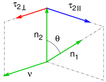
Figure 1: (Color online) The in-plane ($\bm{\tau}_{2\|}$) and out-of-plane ($\bm{\tau}_{2\perp}$) components of the torque $\bm{\tau}_{2}=\bm{\tau}_{2\|}+\bm{\tau}_{2\perp}$ experienced by the FM2 layer. For details, see text.

II.2 In-plane torkance

The basic idea for the in-plane torkance on the FM2 layer rests on the orthogonality relations ${\bf n}_{j}\cdot\bm{\tau}_{j}=0$, $j=1,2$, from which the size of $\bm{\tau}_{2\|}$ can be written as

$$\left({\bf n}_{2}\times\bm{\nu}\right)\cdot\bm{\tau}_{2}=\frac{{\bf n}_{1}\cdot\bm{\tau}_{2}}{\sin\theta}=\frac{{\bf n}_{1}\cdot\bm{\tau}}{\sin\theta},$$ (4)

see Fig. 1. The total torque $\bm{\tau}$, being a full time derivative of $\bm{\sigma}$, in (4) plays a key role in the following treatment.

Our approach applies to systems consisting of the left (${\cal L}$) and the right (${\cal R}$) semiinfinite NM leads with an intermediate region (${\cal I}$) in between; the latter contains both FM layers and the NM spacer of the spin valve. Projection operators on these regions are denoted respectively as $\Pi_{\cal L}$, $\Pi_{\cal R}$ and $\Pi_{\cal I}$; they are mutually orthogonal and satisfy $\Pi_{\cal L}+\Pi_{\cal I}+\Pi_{\cal R}=1$. The Hamiltonian (1) is assumed to be short-ranged (tight-binding), not coupling the two leads, i.e., $\Pi_{\cal L}H\Pi_{\cal R}=0$. The leads are in thermodynamic equilibrium at zero temperature. A general linear response theory can be formulated for a Hermitean operator $Q=Q^{+}$ that is local, i.e., not coupling neighboring parts of the system, so that $Q=\Pi_{\cal L}Q\Pi_{\cal L}+\Pi_{\cal I}Q\Pi_{\cal I}+\Pi_{\cal R}Q\Pi_{\cal R}$. Its time derivative

$$D=-{\rm i}\left[Q,H\right]$$ (5)

is assumed to be localized in ${\cal I}$, i.e., $D=\Pi_{\cal I}D\Pi_{\cal I}$. These properties make it possible to remove the semiinfinite leads from the formalism.

The resulting response coefficient describing the change $\delta{\bar{D}}$ of the thermodynamic average of the quantity $D$ due to an infinitesimal variation $\delta\mu_{\cal L}$ of the chemical potential (Fermi energy) of the ${\cal L}$ lead is given by

$$\frac{\delta\bar{D}}{\delta\mu_{\cal L}}=\frac{1}{2\pi}{\rm Tr}\left\{Q\left(\Gamma_{\cal R}G^{r}\Gamma_{\cal L}G^{a}-\Gamma_{\cal L}G^{r}\Gamma_{\cal R}G^{a}\right)\right\},$$ (6)

where the trace (Tr) and all symbols on the r.h.s. are defined on the Hilbert space of the intermediate region ${\cal I}$, in particular the $Q$ in (6) abbreviates $\Pi_{\cal I}Q\Pi_{\cal I}$. The other symbols in (6) refer to the antihermitean part of the ${\cal L}$ and ${\cal R}$ selfenergies, $\Gamma_{\cal L,R}(E)={\rm i}\left[\Sigma^{r}_{\cal L,R}(E)-\Sigma^{a}_{\cal L,R}(E)\right]$, and to the retarded and advanced propagators

$$G^{r,a}(E)=\left[E-H-\Sigma^{r,a}(E)\right]^{-1},$$ (7)

where $\Sigma^{r,a}(E)=\Sigma^{r,a}_{\cal L}(E)+\Sigma^{r,a}_{\cal R}(E)$ denotes the total selfenergy. Omitted energy arguments in (6) are equal to the Fermi energy of the equilibrium system ($E=E_{F}$).

The proof of (6) is based on non-equilibrium Green’s functions (NGF) for stationary states Haug and Jauho (1996) and it is similar to a previous derivation in Ref. Carva and Turek, 2007. The starting point is an expression for the variation of ${\bar{D}}$,

$$\delta{\bar{D}}=\frac{1}{2\pi}\int_{-\infty}^{\infty}{\rm Tr}\left\{G^{a}(E)DG^{r}(E)\delta\Sigma^{<}(E)\right\}{\rm d}E,$$ (8)

where the variation of the lesser part of the selfenergy at zero temperature is given by

$$\delta\Sigma^{<}(E)=\delta(E-E_{F})\Gamma_{\cal L}(E)\delta\mu_{\cal L}.$$ (9)

The assumed properties of $H$, $Q$ and $D$ lead to a commutation rule for the selfenergy,

$$[Q,\Sigma^{r,a}_{\cal L,R}(E)]=0,$$ (10)

which is proved in the Appendix and which in turn yields a relation

$$G^{a}(E)DG^{r}(E) = {\rm i}\left[G^{a}(E)Q-QG^{r}(E)\right]$$ (11)

$${}+G^{a}(E)Q\Gamma(E)G^{r}(E),$$

where $\Gamma(E)={\rm i}\left[\Sigma^{r}(E)-\Sigma^{a}(E)\right]=\Gamma_{\cal L}(E)+\Gamma_{\cal R}(E)$. The result (6) follows then from an identity for the spectral density operator,

$${\rm i}\left[G^{r}(E)-G^{a}(E)\right]=G^{a}(E)\Gamma(E)G^{r}(E).$$ (12)

Note that the final response coefficient (6) obeys a perfect ${\cal L}$–${\cal R}$ symmetry, i.e., $\delta{\bar{D}}/\delta\mu_{\cal R}=-\delta{\bar{D}}/\delta\mu_{\cal L}$.

It should be emphasized that the derived general result (6) and its perfect ${\cal L}$–${\cal R}$ symmetry are valid only for operators $D$ that can be formulated as a time derivative of a local operator $Q$ according to (5). In the present context of spin valves, this is the case of the usual particle conductance and of the in-plane torkance (see below). The out-of-plane torkance requires a different approach based on the more general relation (8), see Section II.3; its symmetry properties for symmetric spin valves were discussed in details, e.g., in Ref. Ralph and Stiles, 2008.

Application of the derived formula (6) to the transport properties of the spin valves is now straightforward. The usual particle conductance $C$ is based on the operator $Q$ being a projector on a half-space containing, e.g., the ${\cal R}$ lead and an adjacent part of the ${\cal I}$ region. This results in the well-known expression Datta (1995)

$$C=\frac{1}{2\pi}{\rm Tr}\left(\Gamma_{\cal R}G^{r}\Gamma_{\cal L}G^{a}\right),$$ (13)

where atomic units ($e=\hbar=1$) are used. The in-plane torkance $C_{\|}$ on FM2 according to (4) is obtained from $Q={\bf n}_{1}\cdot\bm{\sigma}$ in (6). This yields $C_{\|}=C_{1}/\sin\theta$, where

$$C_{1}=\frac{1}{2\pi}{\rm Tr}\left\{{\bf n}_{1}\cdot\bm{\sigma}\left(\Gamma_{\cal R}G^{r}\Gamma_{\cal L}G^{a}-\Gamma_{\cal L}G^{r}\Gamma_{\cal R}G^{a}\right)\right\}.$$ (14)

The two terms on r.h.s. can be related to spin fluxes on two sides of the FM2 layer. The expression (14) represents our central result. The operators $\Gamma_{\cal L}$ and $\Gamma_{\cal R}$ are localized in narrow regions at the interfaces ${\cal L}/{\cal I}$ and ${\cal I}/{\cal R}$, respectively. The Green’s functions (propagators) for points deep inside the spin valve thus enter neither the conductance (13), nor the in-plane torkance (14).

II.3 Out-of-plane torkance

A similar approach for the out-of-plane torkance on the FM2 layer employs an infinitesimal variation $\delta{\bf n}_{2}$ of its magnetization direction due to a variation $\delta\theta$ of the angle. The FM1 magnetization direction as well as the plane of the two directions ${\bf n}_{1},{\bf n}_{2}$ remain fixed, i.e., $\delta{\bf n}_{1}=\delta\bm{\nu}=0$. This leads to $\delta{\bf n}_{2}=\bm{\nu}\times{\bf n}_{2}\delta\theta$ and from (1) also to

$$H^{\prime}\equiv\frac{\delta H}{\delta\theta}=\gamma_{2}(\bm{\nu}\times{\bf n}_{2})\cdot\bm{\sigma}=\frac{1}{2}\bm{\nu}\cdot\bm{\tau}_{2},$$ (15)

so that the size of $\bm{\tau}_{2\perp}$ coincides (up to factor of 2) with angular derivative of the effective Hamiltonian $H$. The NGF formulation of the out-of-plane torkance rests on relation (8) applied to the operator $D=2H^{\prime}$, see (15), with variation of the selfenergy $\delta\Sigma^{<}(E)$ due to an infinitesimal variation of the chemical potential $\delta\mu_{\cal L}$ given by (9) and similarly for $\delta\Sigma^{<}(E)$ due to the $\delta\mu_{\cal R}$. This yields then response coefficients $C_{\cal L}=\delta\bar{D}/\delta\mu_{\cal L}$ and $C_{\cal R}=\delta\bar{D}/\delta\mu_{\cal R}$ for the out-of-plane torque with respect to chemical potentials of the ${\cal L}$ and ${\cal R}$ leads expressed as

$$C_{\cal L,R}=\frac{1}{\pi}{\rm Tr}\left(H^{\prime}G^{r}\Gamma_{\cal L,R}G^{a}\right).$$ (16)

By employing a simple consequence of (12), $G^{a}=(1+{\rm i}G^{a}\Gamma)G^{r}$, cyclic invariance of trace, angular independence of the selfenergy of NM leads, $\Sigma^{\prime r}=\Sigma^{\prime a}=0$, and the rule $G^{r}H^{\prime}G^{r}=G^{\prime r}$, the response coefficients can be recast into

$$C_{\cal L,R}=\frac{1}{\pi}{\rm Tr}\left\{G^{\prime r}\Gamma_{\cal L,R}\left[1+{\rm i}G^{a}(\Gamma_{\cal L}+\Gamma_{\cal R})\right]\right\},$$ (17)

which contain again only propagators at points close to the ${\cal L}/{\cal I}$ and ${\cal I}/{\cal R}$ interfaces, similarly to (13, 14).

The applied bias has to be identified with the difference $\mu_{\cal L}-\mu_{\cal R}$ and the out-of-plane torkance on FM2 is thus given by $C_{\perp}=(C_{\cal L}-C_{\cal R})/2$. Since the Hamiltonian (1) does not contain spin-orbit interaction, the spin reference system can be chosen such that both unit vectors ${\bf n}_{1}$ and ${\bf n}_{2}$ lie in the $x-z$ plane. This implies that $H$ is essentially time-inversion invariant and it can be represented by a symmetric matrix, $H^{T}=H$; the related quantities $G^{r,a}$ and $\Gamma_{\cal L,R}$ are symmetric as well. As a consequence, the transmission-like terms in $C_{\cal L}$ and $C_{\cal R}$ are the same, i.e., ${\rm Tr}\left(G^{\prime r}\Gamma_{\cal L}G^{a}\Gamma_{\cal R}\right)={\rm Tr}\left(G^{\prime r}\Gamma_{\cal R}G^{a}\Gamma_{\cal L}\right)$. The resulting out-of-plane torkance

$$C_{\perp}=\frac{1}{2\pi}{\rm Tr}\left\{G^{\prime r}[\Gamma_{\cal L}(1+{\rm i}G^{a}\Gamma_{\cal L})-\Gamma_{\cal R}(1+{\rm i}G^{a}\Gamma_{\cal R})]\right\}$$ (18)

contains thus only reflection-like terms.

II.4 Landauer formalism

The Green’s function expression for the conductance (13) can be translated in the language of scattering theory; Arrachea and Moskalets (2006) the counterparts of the torkances (14, 18) are interesting as well. In the present case, propagating states in the ${\cal L}$ and ${\cal R}$ lead will be labelled by $\lambda$ and $\rho$, respectively. Moreover, a spin index $s=\uparrow,\downarrow$ has to be used even for NM leads, since non-collinearity of the spin valve gives rise to full spin dependence of scattering coefficients.

The conductance (13) is given by the Landauer formula $C=(2\pi)^{-1}\sum_{\lambda\rho ss^{\prime}}\left|t_{\rho s^{\prime},\lambda s}\right|^{2}$, where $t_{\rho s^{\prime},\lambda s}$ denotes the transmission coefficient from an incoming state $\lambda s$ into an outgoing state $\rho s^{\prime}$. Landauer (1970) The in-plane torkance coefficient (14) can be written as

$$C_{1}=\frac{1}{2\pi}\sum_{\lambda\rho ss^{\prime}s^{\prime\prime}}({\bf n}_{1}\cdot\bm{\sigma})_{s^{\prime\prime}s^{\prime}}\left(t_{\rho s^{\prime},\lambda s}t^{\ast}_{\rho s^{\prime\prime},\lambda s}-t_{\lambda s^{\prime},\rho s}t^{\ast}_{\lambda s^{\prime\prime},\rho s}\right),$$ (19)

whereas the out-of-plane torkance (18) can be transformed into

$$C_{\perp}=\frac{\rm i}{2\pi}\left(\sum_{\lambda s\lambda^{\prime}s^{\prime}}r^{\prime}_{\lambda^{\prime}s^{\prime},\lambda s}r^{\ast}_{\lambda^{\prime}s^{\prime},\lambda s}-\sum_{\rho s\rho^{\prime}s^{\prime}}r^{\prime}_{\rho^{\prime}s^{\prime},\rho s}r^{\ast}_{\rho^{\prime}s^{\prime},\rho s}\right),$$ (20)

where $r_{\lambda^{\prime}s^{\prime},\lambda s}$ ($r_{\rho^{\prime}s^{\prime},\rho s}$) denote reflection coefficients between states of the ${\cal L}$ (${\cal R}$) lead. This result represents analogy to the Landauer formula and it completes the unified theory of conductances and torkances.

III Results for Cu/Co/Cu/Ni/Cu(001) and their discussion

The developed formalism allows to study properties of spin valves with ultrathin layers, which is yet an experimentally unexplored area; here we demonstrate its use for understanding unexpected features of ab initio results. The results discussed below were obtained using the response of spin currents on both sides of the FM2 layer, Edwards et al. (2005); Theodonis et al. (2006) implemented within the scalar relativistic tight-binding linear muffin-tin orbital (TB-LMTO) method Andersen and Jepsen (1984); Turek et al. (1997) similarly to our previous transport studies. Carva et al. (2006); Carva and Turek (2007) As a case study, spin valves Cu/Co/Cu/Ni/Cu(001) with face-centered cubic (fcc) structure were chosen. All atomic positions were given by an ideal fcc Co lattice with sharp interfaces between the neighboring FM and NM layers. The spin valves discussed below consist of a Co layer of 5 monolayer (ML) thickness separated by a 10 ML thick Cu spacer from a Ni layer of varying thickness, embedded between two semiinfinite Cu leads. Self-consistent calculations within the local spin-density approximation (LSDA) were performed only for collinear spin valves ($\theta=0$ or $\theta=\pi$) while the electronic structure of non-collinear systems was obtained by rotation of the exchange-split potentials of the Co and Ni FM layers. Particular attention has been paid to the convergence of torkances with respect to the number of ${\bf k}_{\|}$ vectors sampling the two-dimensional Brillouin zone (BZ) of the system; in agreement with Ref. Heiliger et al., 2008 we found that reliable values of the out-of-plane torkances require finer meshes than for the in-plane torkances. The presented data were obtained with 6400 ${\bf k}_{\|}$ points in the whole BZ.

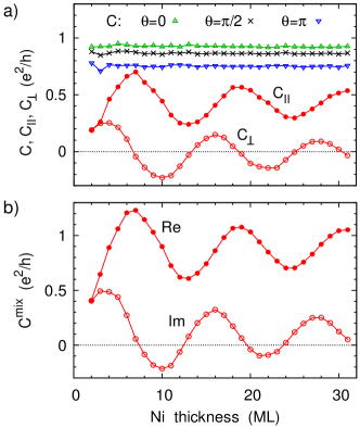
Figure 2: (Color online) Calculated transport coefficients (per interface atom) as functions of Ni thickness: (a) the conductance ($C$) for three values of the angle $\theta$ and the in-plane ($C_{\|}$) and out-of-plane ($C_{\perp}$) Ni-torkances for $\theta=\pi/2$ in spin valves Cu/Co/Cu/Ni/Cu(001), (b) the real (Re) and imaginary (Im) parts of the spin-mixing conductance ($C^{\rm mix}$) of Cu/Ni/Cu(001) systems.

Figure 2a displays the calculated conductances for parallel ($\theta=0$), antiparallel ($\theta=\pi$) and perpendicular ($\theta=\pi/2$) orientations as well as Ni-torkances in the latter case as functions of Ni thickness. The most pronounced feature of the transport coefficients are oscillations with a period of about 12 ML seen in both components of the torkance. These oscillations reflect the perfect ballistic regime of electron transport across the whole spin valve. In addition, they contradict a generally accepted idea of very short magnetic coherence lengths of a few interatomic spacings, or, equivalently, of the spin-transfer torques as an interface property. Brataas et al. (2006); Haney et al. (2007); Heiliger and Stiles (2008); Stiles and Zangwill (2002) Very recently, spin-transfer torques in antiferromagnetic metallic FeMn layers have been investigated theoretically; Xu et al. (2008) it has been shown that the torques are not localized to the interface but are effective over the whole FeMn layer. However, no oscillatory behavior of the total torkance as a function of the layer thickness has been reported. The nature of the predicted oscillations deserves thus detailed analysis, including also a discussion of their stability with respect to structural imperfections and of their absence in the conductance (see Fig. 2a).

Oscillations similar to those in Fig. 2a have recently been obtained for a different quantity of a simpler system, namely for the spin-mixing conductance $C^{\rm mix}$ of epitaxial fcc (001) Ni thin films attached to Cu leads. Carva and Turek (2007) The real and imaginary parts of the complex $C^{\rm mix}$ are related to two components of the spin torque experienced by the FM film due to a spin accumulation in one of the NM leads; Brataas et al. (2006) the calculated values of $C^{\rm mix}$ for the Cu/Ni/Cu(001) system are shown in Fig. 2b. The oscillation periods of the torkance and the spin-mixing conductance are identical which indicates a common origin of both. The physical mechanism behind the $C^{\rm mix}$ oscillations was identified with an interference effect between spin-$\uparrow$ electrons propagating across the Ni film from the ${\cal R}$ lead to the ${\cal L}$ lead and spin-$\downarrow$ electrons propagating backwards. This effect is expressed by a spin-mixing term $\sim{\rm tr}(\Gamma_{\cal R}G^{r}_{\uparrow}\Gamma_{\cal L}G^{a}_{\downarrow})$ in the $C^{\rm mix}$, where the $G^{r,a}_{s}$ ($s=\uparrow,\downarrow$) denote spin-resolved propagators and the trace (tr) does not involve the spin index. Carva and Turek (2007) The particular value of the oscillation period follows from a special shape of the spin-polarized Fermi surface of bulk fcc Ni. Carva and Turek (2007)

The oscillations of $C^{\rm mix}$ have been found fairly stable against Cu-Ni interdiffusion at the interfaces; Carva and Turek (2008) the same stability can be thus expected for the torkance oscillations in the spin valve. The relative stability can be understood as an effect of the large oscillation period ($\sim$ 12 ML): intermixing confined to a very few atomic planes at interfaces reduces the oscillation amplitude rather weakly. This feature contrasts, e.g., sensitivity of the interlayer exchange coupling in magnetic multilayers mediated by a NM Cu(001) spacer with oscillation periods of $\sim$ 2.5 ML and 6 ML, where even a very small amount of interface disorder reduces strongly especially the amplitude of the short period oscillations. Kudrnovský et al. (1996)

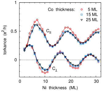
Figure 3: (Color online) Calculated in-plane ($C_{\|}$) and out-of-plane ($C_{\perp}$) Ni-torkances (per interface atom) as functions of Ni thickness in spin valves Cu/Co/Cu/Ni/Cu(001) for $\theta=\pi/2$, 10 ML Cu spacer and for three different Co thicknesses.

Another important aspect of the oscillations of the spin-transfer torques concerns their dependence on the thickness of the polarizing Co layer since ultrathin layers in general might amplify ballistic and interference effects. Figure 3 presents the Ni-torkances in the same Cu/Co/Cu/Ni/Cu(001) spin valves calculated for three different Co thicknesses, namely 5, 15 and 25 ML. It can be seen that the oscillations persist and have the same period in all three cases. Their amplitudes depend slightly on the Co thickness: the initial increase from 5 to 15 Co ML is accompanied by a small reduction (of about 20 %) of the amplitudes whereas further increase from 15 to 25 Co ML does not influence them appreciably. More detailed investigation of the effect of the thickness of the polarizing Co layer, including also the limiting case of spin valves FM1/NM/FM2/NM with a semiinfinite polarizing FM lead, Edwards et al. (2005) is beyond the scope of the present study.

Let us now discuss the absence of oscillations in the conductance (Fig. 2a). We introduce propagators $G^{r,a}_{2}$ of an auxiliary system NM/NM1/NM/FM2/NM, where NM1 denotes the FM1 layer with null exchange splitting. These propagators satisfy $G^{r,a}=G^{r,a}_{2}+G^{r,a}_{2}T^{r,a}_{1}G^{r,a}_{2}$ where the $T^{r,a}_{1}$ denotes the $t$-matrix corresponding to the FM1 exchange splitting $\gamma_{1}$ in (1). The conductance (13) can be then rewritten as $C=(2\pi)^{-1}{\rm Tr}(\Gamma_{\cal R}G^{r}_{2}\Delta_{\cal L}G^{a}_{2})$, where $\Delta_{\cal L}=(1+T^{r}_{1}G^{r}_{2})\Gamma_{\cal L}(1+G^{a}_{2}T^{a}_{1})$ represents an operator localized at the FM1 layer, i.e., at the left end of the FM2 layer. The latter trace can be most easily evaluated using the spin quantization axis parallel to the FM2 magnetization direction ${\bf n}_{2}$. Since the propagators $G^{r,a}_{2}$ are now diagonal in the spin index $s$ and the operator $\Gamma_{\cal R}$ is spin-independent, the conductance does not contain spin-mixing terms, i.e., terms $\sim{\rm tr}(\Gamma_{\cal R}G^{r}_{2,s}\Delta_{{\cal L},ss^{\prime}}G^{a}_{2,s^{\prime}})$ for $s\neq s^{\prime}$ that result in interference effects involving different spin channels. For the torkance, however, the extra factor ${\bf n}_{1}\cdot\bm{\sigma}$ in (14) provides the necessary spin mixing responsible for the oscillations, in full analogy to oscillations of the spin-mixing conductance.

A recent study of spin-transfer torques in a tunnel junction Cu/Fe/MgO/Fe/Cu has predicted torkance and conductance oscillations with Fe thickness with a period $\sim$ 2 ML. Heiliger and Stiles (2008) These oscillations were ascribed to quantum well states in the majority spin of the Fe layer, i.e., to interference effects in a single spin channel. The oscillations in the Cu/Co/Cu/Ni/Cu system—manifested only in the torkance—have thus a clearly different origin.

IV Conclusion

We have addressed two important aspects of spin-transfer torques in non-collinear spin valves with ultrathin layers. First, we have shown that the in-plane and out-of-plane torkance on one FM layer can be expressed by means of the transmission and reflection coefficients, respectively, of the whole spin valve, in close analogy to the Landauer formula for the ballistic conductance. Second, a novel oscillatory behavior for Ni-based systems has been predicted due to the mixed spin channels. The oscillations with Ni thickness are reasonably stable with respect to interface imperfections of real samples; however, they are not present in the conductance but can be observed only in the Ni-torkance. The torkance oscillations prove that the spin-transfer torques in ballistic spin valves are closely related to properties of their components, in particular to the spin-mixing conductances of individual ferromagnetic layers.

*

Appendix A Proof of the commutation rule for selfenergy

The proof of the commutation rule (10) rests on assumed properties of the operators $H$, $Q$, $D$ (defined in the Hilbert space of the total system) and of the projectors $\Pi_{\cal L}$, $\Pi_{\cal R}$, $\Pi_{\cal I}$, see the beginning of Section II.2. Let as abbreviate projections of any operator $X$ ($X=H,Q,D$) as $\Pi_{\cal I}X\Pi_{\cal I}\equiv X_{\cal II}$, $\Pi_{\cal I}X\Pi_{\cal L}\equiv X_{\cal IL}$, etc. The assumed property of $Q$, namely $Q=Q_{\cal LL}+Q_{\cal II}+Q_{\cal RR}$, a consequence of the localization of $D$ in ${\cal I}$, namely $D_{\cal IL}=0$ and $D_{\cal LI}=0$, and the orthogonality of the projectors $\Pi_{\cal L}$, $\Pi_{\cal R}$, $\Pi_{\cal I}$ lead to identities

$$Q_{\cal II}H_{\cal IL}=H_{\cal IL}Q_{\cal LL},\quad Q_{\cal LL}H_{\cal LI}=H_{\cal LI}Q_{\cal II}.$$ (21)

Similarly, a commutation rule

$$Q_{\cal LL}H_{\cal LL}=H_{\cal LL}Q_{\cal LL}$$ (22)

can easily be obtained from $D_{\cal LL}=0$.

The left selfenergy is given explicitly by

$$\Sigma^{r,a}_{\cal L}(E)=H_{\cal IL}{\cal G}^{r,a}_{\cal L}(E)H_{\cal LI},$$ (23)

where the ${\cal G}^{r,a}_{\cal L}(E)$ denotes the retarded and advanced propagator of the isolated left lead. The relation (22) implies immediately a commutation rule

$$Q_{\cal LL}{\cal G}^{r,a}_{\cal L}(E)={\cal G}^{r,a}_{\cal L}(E)Q_{\cal LL};$$ (24)

its application together with (21, 23) leads to identities

$$Q_{\cal II}\Sigma^{r,a}_{\cal L}(E)=Q_{\cal II}H_{\cal IL}{\cal G}^{r,a}_{\cal L}(E)H_{\cal LI}$$ (25)

$$= H_{\cal IL}Q_{\cal LL}{\cal G}^{r,a}_{\cal L}(E)H_{\cal LI}=H_{\cal IL}{\cal G}^{r,a}_{\cal L}(E)Q_{\cal LL}H_{\cal LI}$$

$$= H_{\cal IL}{\cal G}^{r,a}_{\cal L}(E)H_{\cal LI}Q_{\cal II}=\Sigma^{r,a}_{\cal L}(E)Q_{\cal II},$$

which are equivalent to the commutation rule (10) for the left selfenergy. The proof for the right selfenergy is similar and therefore omitted.

References

- Slonczewski (1996) J. C. Slonczewski, J. Magn. Magn. Mater. 159, L1 (1996).
- Berger (1996) L. Berger, Phys. Rev. B 54, 9353 (1996).
- Myers et al. (1999) E. B. Myers, D. C. Ralph, J. A. Katine, R. N. Louie, and R. A. Buhrman, Science 285, 867 (1999).
- Katine et al. (2000) J. A. Katine, F. J. Albert, R. A. Buhrman, E. B. Myers, and D. C. Ralph, Phys. Rev. Lett. 84, 3149 (2000).
- Brataas et al. (2006) A. Brataas, G. E. W. Bauer, and P. J. Kelly, Phys. Rep. 427, 157 (2006).
- Slonczewski and Sun (2007) J. C. Slonczewski and J. Z. Sun, J. Magn. Magn. Mater. 310, 169 (2007).
- Theodonis et al. (2006) I. Theodonis, N. Kioussis, A. Kalitsov, M. Chshiev, and W. H. Butler, Phys. Rev. Lett. 97, 237205 (2006).
- Heiliger and Stiles (2008) C. Heiliger and M. D. Stiles, Phys. Rev. Lett. 100, 186805 (2008).
- Edwards et al. (2005) D. M. Edwards, F. Federici, J. Mathon, and A. Umerski, Phys. Rev. B 71, 054407 (2005).
- Wang et al. (2008) S. Wang, Y. Xu, and K. Xia, Phys. Rev. B 77, 184430 (2008).
- Haney et al. (2007) P. M. Haney, D. Waldron, R. A. Duine, A. S. Núñez, H. Guo, and A. H. MacDonald, Phys. Rev. B 76, 024404 (2007).
- Waintal et al. (2000) X. Waintal, E. B. Myers, P. W. Brouwer, and D. C. Ralph, Phys. Rev. B 62, 12317 (2000).
- Landauer (1970) R. Landauer, Philosophical Magazine 21, 863 (1970).
- Datta (1995) S. Datta, Electronic Transport in Mesoscopic Systems (Cambridge University Press, 1995).
- Haug and Jauho (1996) H. Haug and A.-P. Jauho, Quantum Kinetics in Transport and Optics of Semiconductors (Springer, Berlin, 1996).
- Carva and Turek (2007) K. Carva and I. Turek, Phys. Rev. B 76, 104409 (2007).
- Ralph and Stiles (2008) D. C. Ralph and M. D. Stiles, J. Magn. Magn. Mater. 320, 1190 (2008).
- Arrachea and Moskalets (2006) L. Arrachea and M. Moskalets, Phys. Rev. B 74, 245322 (2006).
- Andersen and Jepsen (1984) O. K. Andersen and O. Jepsen, Phys. Rev. Lett. 53, 2571 (1984).
- Turek et al. (1997) I. Turek, V. Drchal, J. Kudrnovský, M. Šob, and P. Weinberger, Electronic Structure of Disordered Alloys, Surfaces and Interfaces (Kluwer, Boston, 1997).
- Carva et al. (2006) K. Carva, I. Turek, J. Kudrnovský, and O. Bengone, Phys. Rev. B 73, 144421 (2006).
- Heiliger et al. (2008) C. Heiliger, M. Czerner, B. Y. Yavorsky, I. Mertig, and M. D. Stiles, J. Appl. Phys. 103, 07A709 (2008).
- Stiles and Zangwill (2002) M. D. Stiles and A. Zangwill, Phys. Rev. B 66, 014407 (2002).
- Xu et al. (2008) Y. Xu, S. Wang, and K. Xia, Phys. Rev. Lett. 100, 226602 (2008).
- Carva and Turek (2008) K. Carva and I. Turek, Physica Status Solidi A 205, 1805 (2008).
- Kudrnovský et al. (1996) J. Kudrnovský, V. Drchal, I. Turek, M. Šob, and P. Weinberger, Phys. Rev. B 53, 5125 (1996).