Phase ordering and universality for continuous symmetry models on graphs

Abstract

We study the phase-ordering kinetics following a temperature quench of $O(\cal N)$ continuous symmetry models with ${\cal N}=3$ and ${\cal N}=4$ on graphs. By means of extensive simulations, we show that the global pattern of scaling behaviors is analogous to the one found on usual lattices. The exponent $a_{\chi}$ for the integrated response function and the exponent $z$, describing the growing length, are related to the large scale topology of the networks through the spectral dimension and the fractal dimension alone, by means of the same expressions provided by the analytic solution of the $\cal N\to\infty$ limit. This suggests that the large-$N$ value of these exponents could be exact for every ${\cal N}\geq 2$.

1 Introduction

A ferromagnetic system quenched from a high temperature disordered state to an ordered phase with broken ergodicity evolves via phase-ordering dynamics. In the late stage of growth, the correlation of the order parameter between sites $i,j$ at times $s,t$ can be expressed as the sum of two terms [1]

$${\cal C}_{ij}(t,s)={\cal C}^{st}_{ij}(t-s)+{\cal C}^{ag}_{ij}(t,s).$$ (1)

The first term describes the contribution provided by degrees of freedom which in the interval $[s,t]$ are not interested by non-equilibrium effects, such as the passage of topological defects, while the second contains the non-equilibrium information. Analogously, also the integrated response function, or zero field cooled magnetization, measured on site $i$ at time $t$ after a perturbation has been switched on in $j$ from time $s$ onwards, takes an analogous addictive form [2]

$$\chi_{ij}(t,s)=\chi^{st}_{ij}(t-s)+\chi^{ag}_{ij}(t,s).$$ (2)

On regular lattices, due to space homogeneity and isotropy, correlation and response function depend only on the distance $r$ between $i$ and $j$. One has, therefore, ${\cal C}_{ij}(t,s)={\cal C}(r,t,s)$, and similarly for $\chi_{ij}(t,s)$.

The non-equilibrium behaviour is characterized by the dynamical scaling symmetry, a self-similarity where time acts as a length rescaling. When scaling holds, the states sequentially probed by the system are statistically equivalent provided lengths are measured in units of the characteristic length scale $L(t)$, which increases in time. All the time dependence enters through $L(t)$, and the aging parts in Eqs. (1,2) take a scaling form in terms of rescaled variables [1] $x=r/L(s)$ and $y=L(t)/L(s)$

$${\cal C}^{ag}(r,t,s)=\tilde{\cal C}(x,y),$$ (3)

$$\chi^{ag}(r,t,s)=s^{-a_{\chi}}\tilde{\chi}(x,y).$$ (4)

The characteristic length usually grows according to a power law

$$L(t)\sim t^{1/z}.$$ (5)

Interestingly, non-equilibrium exponents are expected to be universal, namely to depend only on a restricted set of parameters. On regular lattices, where a substantial understanding of the dynamics has been achieved by means of exact solutions, approximate theories and numerical simulations [3], these exponents depend only on the space dimensionality, the number of components ${\cal N}$ of the order parameter and the conservation laws of the dynamics. In this paper we will consider primarily $z$ and $a_{\chi}$. It is known [3], that $z$ depends only on the conservation laws, being $z=2$ in the case of a non conserved order parameter considered in this paper. Regarding $a_{\chi}$, for continuous symmetry models (${\cal N}>1$) with non-conserved order parameter, it was conjectured in  [4] to obey

$$a_{\chi}=\left\{\begin{array}[]{ll}\frac{d-2}{2}\qquad$for$\qquad d<4\\ 1\qquad$with log corrections for$\qquad d=4\\ 1\qquad$for$\qquad d>4.\end{array}\right.$$ (6)

Let us notice that these exponents share the property of being ${\cal N}$-independent. Their value therefore can be computed in the soluble large-${\cal N}$ model [5]. The reference framework of a soluble theory is a great advantage in the study of phase-ordering on networks or inhomogeneous graphs considered in this paper. In fact our understanding of these systems is largely incomplete, although examples can be found in disordered materials, percolation clusters, glasses, polymers, and bio-molecules, and are also present in interdisciplinary studies, ranging from economics to chemistry and social sciences [7]. The aim of this paper is to investigate if also on networks the non-equilibrium dynamics of statistical models takes a scaling structure, and its universality features. Moreover, it is interesting to understand which topological indices of the graph play the role of the euclidean dimension $d$ on regular lattices in determining universal quantities. We will restricted our attention to physical graphs [8]: These are networks with the appropriate topological features to represent real physical structures, namely they are embeddable in a finite dimensional space and have bounded degree.

Equilibrium properties of models defined on physical graphs, and in particular the relevance of their topology, are quite well understood. As far as systems with continuous symmetry are concerned, such as $O({\cal N})$ models (${\cal N}\geq 2$), a unique parameter, the ”spectral dimension” $d_{s}$, encodes the relevant large scale topological features of the network and regulates the critical properties. $d_{s}$ is related to the low eigenvalues behaviour of the density of state of the Laplacian operator [9], and can be considered for these models as the topological indicator replacing the Euclidean dimension $d$ on graphs: The spectral dimension univocally determines the existence of phase transitions [10] and controls critical behaviours [11], much in the same way as the Euclidean dimension $d$ does on usual translation invariant lattices.

Regarding non-equilibrium, in the large-${\cal N}$ model it was shown [12, 13] that the general framework of scaling behaviour discussed above is maintained on generic graphs. In particular the topology of the network enters the exponent $z$ only through the fractal dimension $d_{f}$ and the spectral dimension $d_{s}$,

$$z=2d_{f}/d_{s},$$ (7)

while $a_{\chi}$ depends only on the spectral dimension obeying (6) with $d_{s}$ occurring in place of $d$.

In this paper we want to complement the large-${\cal N}$ analysis by studying the phase-ordering kinetics of some $O({\cal N})$ vector models with finite ${\cal N}$ on a class of physical graphs. We will consider geometrical fractals without phase transition at finite temperature, such as the Sierpinski gasket or the T-fractal, and others structures, obtained by direct products among graphs [8], which on the contrary feature a phase transitions at a finite temperature $T_{c}$. Our simulations of these systems evolving with relaxational dynamics (non-conserved order parameter) show that, for ${\cal N}=3$ and ${\cal N}=4$, the dynamical exponents $z$ and $a_{\chi}$ are correctly predicted by the large-${\cal N}$ model and then depend only on the fractal and spectral dimensions $d_{f},d_{s}$. This suggests that in presence of scaling these exponents take the same value for any ${\cal N}\geq 2$, much in the same way as it happens on euclidean lattices.

This paper is organized as follows: In Sec. 2 we introduce the physical graphs giving a definition of fractal and spectral dimension. In Sec. 3 we define the $O({\cal N})$ models that will be considered in the simulations. We also introduce the basic observables, and discuss the numerical techniques. In Sec. 4 we present our results for different structures. Sec. 5 contains a final discussion and the conclusions.

2 Physical Graphs

A graph (network) $\cal G$ is a discrete structure defined by a set of sites $i$ connected pairwise by unoriented links (edges) $\{i,j\}$. The chemical distance $r_{i,j}$, i.e. the number of links in the shortest path connecting sites $i$ and $j$, naturally defines on $\cal G$ a metric. Van Hove spheres , allowing to explore large scales of the graph, can be constructed using this metric. The van Hove sphere ${\cal S}_{o,r}$ of radius $r$ and center $o$ is the sub-graph of $\cal G$ composed by the sites whose distance from $o$ is smaller than $r+1$. Calling $N_{o,r}$ the number of sites in ${\cal S}_{o,r}$, the fractal dimension of the graph is defined by its asymptotic behaviour at large scales

$$N_{o,r}\sim r^{d_{f}}$$ (8)

where $\sim$ denotes the behaviour for large $r$. In the following we will consider only physical graphs embeddable in a finite dimensional space ($d_{f}$ is well defined and finite). Moreover we require that the degree $z_{i}$ (number of neighbours of the site $i$) is bounded.

Algebraic graph theory provides powerful tools for the description of the topology of generic networks, by means of characteristic matrices. The adjacency matrix $A_{i,j}$ of a graph has entries equal to $1$ if $i$ and $j$ are neighbouring sites ($\{i,j\}$ is a link) and $A_{i,j}=0$ otherwise. The Laplacian matrix $\Delta_{i,j}$ is defined as

$$\Delta_{i,j}=\delta_{i,j}z_{i}-A_{i,j}$$ (9)

where $z_{i}=\sum_{j}A_{i,j}$ is the degree of $i$. Interestingly, $\Delta_{i,j}$ is the generalization to graphs of the usual Laplacian operator of Euclidean structures [8]. In particular its spectrum is positive and the constant vector is the only eigenvector of eigenvalue zero. Moreover, on physical graphs the spectral density $\rho(l)$ of $\Delta_{i,j}$, is expected to behave as [9]

$$\rho(l)\sim l^{d_{s}/2-1}$$ (10)

where $\sim$ denotes the behaviour for small $l$’s. Eq. (10) defines the spectral dimension $d_{s}$ of the physical graph.

In order to build graphs of larger dimensions we introduce the direct product between graphs. Given $\cal G$ and $\cal H$ the direct product ${\cal G}\times{\cal H}$ is a graph whose sites are labelled by a pair $(i,j)$ with $i$ and $j$ belonging to $\cal G$ and $\cal H$ respectively. $(i,j)$ and $(i^{\prime},j^{\prime})$ are neighbour sites in ${\cal G}\times{\cal H}$ if $i=i^{\prime}$ and $\{j,j^{\prime}\}$ is a link of $\cal H$, or if $j=j^{\prime}$ and $\{i,i^{\prime}\}$ is a link of $\cal G$. A basic properties of ${\cal G}\times{\cal H}$ is that, calling $d_{s}^{\cal G}$ and $d_{f}^{\cal G}$ the dimensions of the graph $\cal{G}$, one has [8]

$$d_{s}^{{\cal G}\times{\cal H}}=d_{s}^{{\cal G}}+d_{s}^{{\cal H}}~{}~{}~{}~{}~{}~{}~{}d_{f}^{{\cal G}\times{\cal H}}=d_{f}^{{\cal G}}+d_{f}^{{\cal H}}~{}~{}~{}~{}~{}~{}~{}$$ (11)

i.e. the spectral and fractal dimensions of the product graph are the sum of the dimensions of the original graphs.

In the simulations, we will consider models defined on graphs with known $d_{s}$ and $d_{f}$ in order to verify the relevance of these dimensions, describing the large scale topology, on phase ordering. In particular, we focus on two finitely ramified fractals [14] with $d_{s}<2$, the T-fractal and the Sierpinski gasket, whose fractal and spectral dimensions can be analytically evaluated by means of exact renormalizations [15], yielding $d_{f}=\log(3)/\log(2)$, $d_{s}=\log(9)/\log(6)$ and $d_{f}=\log(3)/\log(2)$, $d_{s}=\log(9)/\log(5)$ respectively. Moreover, in order to explore the region between $d=2$ and $d=3$, we also consider the graphs obtained from the product of two gaskets and two T-fractals, which both have spectral dimensions $2<d_{s}<3$ .

Figure 1: The finitely ramified fractals considered in the paper.

3 The Model

The Hamiltonian of $O({\cal N})$ spin systems on a graph is given by:

$$H_{0}[\vec{\sigma}]=-J\sum_{i,j}^{N}A_{i,j}\vec{\sigma}_{i}\cdot\vec{\sigma}_{j}$$ (12)

where $|\vec{\sigma}_{i}|=1$ are unitary $\cal N$-component vectors, and $N$ is the number of sites in the network. In the following we will set $J=1$. Phase ordering is obtained by evolving an initially fully disordered configuration with a dynamics at a temperature $T$ where the system presents an ordered phase at equilibrium. In the following we will consider quenches to $T=0$. This guarantees that the dynamics is of the phase-ordering type even for those systems with $d_{s}\leq 2$, namely without phase transition at finite temperature.

Phase ordering can be characterized by the correlation function, defined as

$${\cal C}_{ij}(t,s)=\langle\vec{\sigma}_{i}(t)\cdot\vec{\sigma}_{j}(s)\rangle-\langle\vec{\sigma}_{i}(t)\rangle\cdot\langle\vec{\sigma}_{j}(s)\rangle$$ (13)

Recalling Eqs. (1,3), the non-equilibrium scaling properties are encoded in the aging part ${\cal C}_{ij}^{ag}(t,s)$ which, in turn, can be obtained by subtracting the equilibrium contribution $C_{ij}^{st}(t,s)$ from the whole correlation ${\cal C}_{ij}(t,s)$. Notice however that at $T=0$, ${\cal C}_{ij}^{st}(t,s)$ vanishes and hence ${\cal C}_{ij}^{ag}(t,s)={\cal C}_{ij}(t,s)$. We will drop therefore the superscript $ag$ from the correlation function in the following. In order to simplify the analysis one usually restricts the attention to ${\cal C}_{ij}(t,t)$, namely the equal time correlation function, or to the autocorrelation function ${\cal C}_{ii}(t,s)$. On lattices ${\cal C}_{ij}(t,t)=G(r,t)$ is a function of the euclidean distance $r$ between $i$ and $j$ which, according to Eq. (3) scales as

$$G(r,t)=g(r/L(t))$$ (14)

This allows one to extract $L(t)$ as, for instance, the half-height width of $G(r,t)$. Concerning the autocorrelation function, on lattices it does not depend on $i$, due to translational invariance, so that ${\cal C}_{ii}(t,s)=C(t,s)$ with, following Eq. (3), the scaling form

$$C(t,s)=f(y)\sim y^{-\lambda},$$ (15)

where $\lambda$ depends both on $d$ and on $\cal N$ [3].

When phase-ordering occurs on graphs one has the additional feature of the dependence of ${\cal C}_{ij}(t,t)$ on $i$ and $j$ (and ${\cal C}_{ii}(t,s)$ on $i$), complicating the analysis and hindering the scaling properties. Therefore, in order to simplify the study, we will resort in the following to particular correlations, with a transparent physical meaning, which where shown in [13, 16] to be useful in detecting scaling properties. More precisely, for the equal time correlation function, on the Sierpinski gasket and on the T-fractal we will compute it restricting $i$ and $j$ on the baseline of the structure (see Fig. 1), as this procedure allows to soften the log-periodic oscillations characteristic of deterministic fractals [17] and gives the best results for the scaling plots, as will be shown in Sec. 4. Regarding the autocorrelation function we will consider its spatial average ${1\over N}\sum_{i=1}^{N}{\cal C}_{ii}(t,s)$, in order to obtain the best statistic. For simplicity these quantities will be denoted as $G(r,t)$ and $C(t,s)$ in analogy to their counterparts on lattices.

The response of the system to an external field can be studied introducing the susceptibility

$$\chi_{ij}(t,s)=\lim_{h\to 0}{1\over h}\langle\vec{\sigma}_{i}(t)\rangle_{h_{j}(s)}\cdot\vec{n}_{j}$$ (16)

where $\langle\vec{\sigma}_{i}(t)\rangle_{h_{j}(s)}$ denotes the expectation value at time $t$ of the spin $\vec{\sigma}_{i}$ when a field $\vec{h}_{j}=h\vec{n}_{j}$ ($\vec{n}_{j}$ being a unitary vector), changing the Hamiltonian to $H[\vec{\sigma}]=H_{0}[\vec{\sigma}]-\vec{\sigma}_{j}\cdot\vec{h}_{j}$ is switched on from time $s<t$ onwards on site $j$. Differently from what happens for ${\cal C}_{ij}(t,s)$, the equilibrium contribution to $\chi_{ij}(t,s)$ does not vanish. Then, in order to isolate the scaling part $\chi_{ij}^{ag}(t,s)$, according to Eq. (2) one has to subtract $\chi_{ij}^{st}(t-s)$ from the whole response measured during the quench. $\chi_{ij}^{st}(t-s)$ can be numerically evaluated as the response of a system prepared initially in the equilibrium state at $T=0$, namely with all the spins aligned. Actually, if one does this the system starts to evolve as soon as a small field $h>0$ is switched on even if $T=0$, originating a non-vanishing response. Considering, for simplicity, the autoresponse $\chi(t,s)=\chi_{ii}(t,s)$, on lattices, from Eq. (4) one finds

$$\chi^{ag}(t,s)=s^{-a_{\chi}}h(y)$$ (17)

with $a_{\chi}$ depending only on $d$ according to Eq. (6). On networks the response function is site dependent, so, similarly to what done for the autocorrelation function, we will consider the spatially averaged quantity ${1\over N}\sum_{i=1}^{N}\chi_{ii}(t,s)$ which will be denoted as $\chi(t,s)$.

Zero temperature dynamics can be implemented in different ways. For example one can set $T=0$ in a Metropolis updating rule. A convenient choice adopted in this paper consists in aligning a randomly chosen spin $\vec{\sigma}_{i}$ with the local field, i.e. the spin $\vec{\sigma}_{i}$ is turned into

$$\vec{\sigma}_{i}\to\vec{\sigma}_{i}^{\prime}=|h|\vec{n}_{i}+\sum_{j}A_{i,j}\vec{\sigma}_{j}.$$ (18)

With this choice, at each move the local energy is minimized. Such a simple updating rule proves to be very efficient, on networks and lattices as well. For instance it allows to reproduce easily the analytically known behaviour of the $O(2)$ model in one-dimension [18], whereas the Metropolis rule fails due to extremely long transients (see Appendix for details). Notice that in one-dimensional $O(2)$ model scaling is violated, and our hypothesis on dynamical exponents does not hold.

The scope of this study being the analysis of the behaviour of finite ${\cal N}$ models, the less numerically demanding case to start with would naturally be the $O(2)$ model. However, as discussed in the Appendix, the dynamics of this model is pinned on self-similar graphs such as the Sierpinski gasket or the T-fractal considered here. Then, in order to study the phase ordering kinetics in this case, one should allow the system to depin by quenching to a small but finite temperature. Since the above mentioned structures, however, are disordered at any finite temperature, in order to recover true phase-ordering one should then let $T\to 0$, in the same way as for phase-ordering in the one-dimensional Ising model with Kawasaki dynamics [19]. Since this procedure is very numerically demanding, hereafter we will focus on the next simplest cases, namely with ${\cal N}=3$ and ${\cal N}=4$ (the latter restricted to the Sierpinski gasket). Performing extensive numerical simulation of these models on different self-similar graphs, we show that phase ordering exhibits dynamical scaling, similarly to what is known on lattices, in any case. In particular, the correlation length grows according to Eq. (5) and the two time correlation and response functions scale as (15) and (17). We also find that the exponents $z$ and $a_{\chi}$ are well consistent with their large-${\cal N}$ value. This suggests that also on graphs, as on lattices, these exponent do not depend on ${\cal N}$, and that their value can be predicted by the solution of the large-${\cal N}$ model for every scaling system with ${\cal N}\geq 2$.

4 Results

In the numerical simulations we considered the Sierpinski gasket, the T-fractal, and the graphs obtained by a direct product of two gaskets and of two T-fractals. The number of sites $N$ of the structures is 2391486, 1549324,10771524 and 4787344 respectively. A time-step is made of $N$ elementary Montecarlo moves (18). The data are obtained by averaging over at least 500 dynamical realizations, each with a different random initial condition. For the calculus of $\chi(s,t)$ a different random field $\vec{n}_{i}$ is applied in each run. To evaluate the limit $h\to 0$ in Eq. (16), we have simulated systems with small external fields $h$ and then we have verified that $\chi(t,s)$ is independent of $h$ (e.g. comparing systems with field $h$ and $h/2$). In our simulations $h$ varies between $10^{-1}$ and $10^{-3}$.

In Figure 2 we show the behaviour of the equal time correlation function $G(r,t)$ defined in Sec. 3 for the Sierpinski gasket. The Figure evidences an excellent scaling, in the form expected from Eq. (14). Quite surprisingly, the scaling is very good even for very short times ($t$ ranges from 8 to 46600) evidencing the efficiency of the dynamics considered. Analogous results were obtained for the T-fractal. In Figure 3 we plot the growth of $L(t)$ as a function of time, finding a very good agreement with the asymptotic behaviour $L(t)\sim t^{d_{s}/(2d_{f})}$ (namely $t^{0.431}$ and $t^{0.387}$ for the Sierpinski gasket and the T-fractal respectively). We note that superimposed to the expected behaviour there are small log-periodic oscillations, typical of fractal structures [17]. If the average of the correlation function is not restricted on the baseline of the structure, but is taken on the whole fractal, the log-periodic oscillations are more evident, as shown in Figure 3 for the Sierpinski gasket, while keeping the same slope for the $L(t)$. If this average procedure is used, it is more difficult to extract the scaling behaviour of the correlation function.

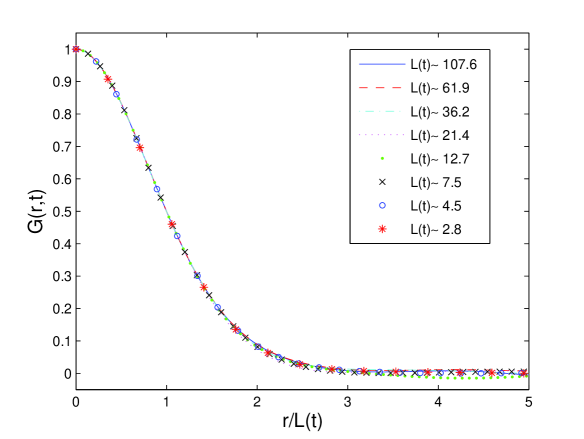
Figure 2: Scaling of $G(r,t)$ evaluated on the baseline of a Sierpinski gasket.

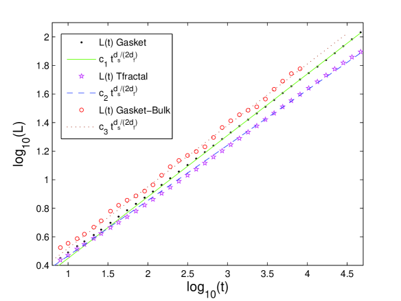
Figure 3: Growth of $L(t)$ as a function of time, anomalous diffusive behaviour $L(t)\propto t^{1/z}$ is well verified. For distances evaluated along the baseline, best fits yield $1/z=0.42\pm 0.01$ and $1/z=0.39\pm 0.01$ for the Sierpinski gasket and the T-fractal, respectively, very well consistent with the large-${\cal N}$ behaviour $1/z={d_{s}/(2d_{f})}$ in both cases. For the Sierpinski Gasket we also plot $L(t)$, evaluated averaging over sites belonging to the bulk of the structure. The value of the exponent does not change, but the log-periodic oscillations are much larger.

Let us now turn to the response function. It has been analyzed as follows: After computing $\chi^{ag}(t,s)$ by subtracting $\chi^{st}(t,s)$ to the full non-equilibrium response, as explained in Sec. 3, we fix the ratio $y=t/s$ and plot $\chi^{ag}(t,s)$ versus $s$ (Fig. 4). In doing so we obtain, from (17), an estimate for $a_{\chi}$ from the slope of the plot. As illustrated in Fig. 4, both for the Sierpinski gasket and for the T-fractal the value of $a_{\chi}$ is consistent with $d_{s}/2-1$ (namely $a_{\chi}=-0.317$ for the Sierpinski gasket and $a_{\chi}=-0.387$ for the T-fractal) i.e. the analytic expression obtained in the ${\cal N}\to\infty$ case (except for the smaller values of $t/s$, as we will discuss below). Finally, we verified the scaling relation (17) by plotting $s^{a_{\chi}}\chi^{ag}(t,s)$ versus $t/s$ for different values of $s$ and checking for data collapse, as shown for the Sierpinski gasket in Fig. 5. The collapse is good for $t/s\gtrsim 5$, whereas it is poor for smaller values of $t/s$. This can be interpreted as due to finite-$s$ preasymptotic corrections, which are more effective at small $t/s$, similarly to what observed on lattices [4, 6]. Analogous result can be obtained for the T-fractal. Let us stress the particular feature of the cases with $d_{s}<2$ of $\chi^{st}(t-s)$ (and hence $\chi(t,s)$) scaling itself as $s^{-a_{\chi}}\tilde{h}(t/s)$, with the same exponent $a_{\chi}$ of $\chi^{ag}(t,s)$ and with a scaling function $\tilde{h}(y)$ that, although different from $h(y)$, has the same asymptotic behaviour $\tilde{h}(y)\simeq y^{-a_{\chi}}$ for $y\gg 1$. In this case, therefore, one gets the same information on the exponents from $\chi(t,s)$, $\chi^{ag}(t,s)$ and $\chi^{st}(t-s)$. The situation is different for $d_{s}>2$. Here the stationary term converges to the finite equilibrium susceptibility, $\lim_{t\to\infty}\chi^{st}(t-s)=\chi_{eq}$, whereas $\chi^{ag}(t,s)$ scales with a positive $a_{\chi}$ (see below). In this case, therefore, $\chi(t,s)$ is dominated by $\chi^{st}(t/s)$ and the subtraction of $\chi^{st}(t/s)$ is necessary in order to make the scaling of the aging part manifest. In Fig. 6 we evaluate the exponent $a_{\chi}$, following the procedure discussed above, both for the product of gaskets and for the product of T-fractals. Also in this case we get a very good agreement with the expected behaviour $a_{\chi}=d_{s}/2-1$ (namely $a_{\chi}=0.365$ and $a_{\chi}=0.226$ for the product of gaskets and the product of T-fractals respectively).

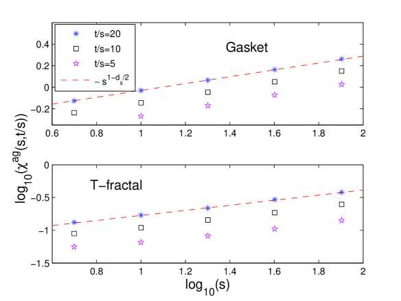
Figure 4: Estimate of the exponent $a_{\chi}$ for the Sierpinski gasket and the T-fractal (see text). Best fits yield $a_{\chi}=-0.32\pm 0.01$ for the Sierpinski gasket and $a_{\chi}=-0.38\pm 0.01$ for the T-fractal. In both cases these values are consistent with the hypothesis $a_{\chi}=d_{s}/2-1$.

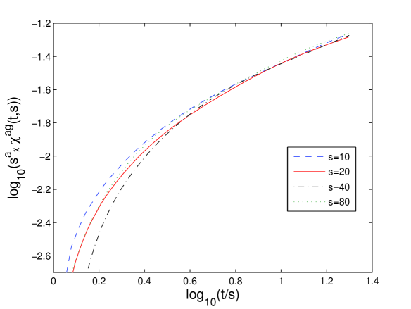
Figure 5: Scaling of the function $\chi^{ag}(t,s)$ on the Sierpinski gasket. At large time ratio, a good agreement with the scaling hypothesis (17) is verified for $s\geq 10$.

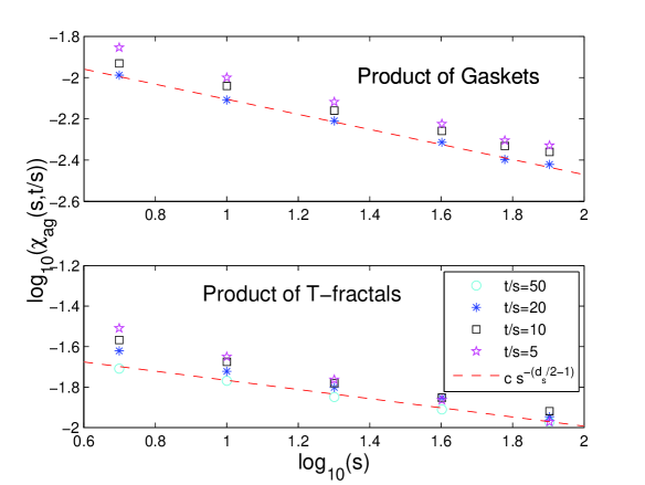
Figure 6: Estimate of the exponent $a_{\chi}$ for the product of Sierpinski gaskets and the product of T-fractals. Best fits yield $a_{\chi}=0.36\pm 0.01$ for the product of Sierpinski gaskets and $a_{\chi}=0.22\pm 0.01$ for the product of T-fractals. In both cases a good agreement with the large-${\cal N}$ value is evidenced. Notice that in the first case the asymptotic regime is reached much earlier than in the second one.

In order to provide a further check on dynamical scaling, we have considered also the two-time correlation function $C(t,s)$ introduced in Sec. 3. The scaling relation (15) is well verified, as shown in Fig. 7 for the Sierpinski gasket. A residual correction, due to the finite values of $t_{w}$ can be observed for large $t/t_{w}$, similarly to what is known in lattices [20]. The quality of the scaling improves by increasing $t_{w}$, with the curves for $t_{w}=40,80,160$ almost collapsing, as expected. Similar results were found for the T-fractal.

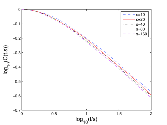
Figure 7: Scaling of the two time correlation function $C(s,t)$. A good agreement with the hypothesis $C(s,t)=h(s/t)$ is found.

Up to now, by focusing on the case ${\cal N}=3$, we have shown that the global pattern of behaviours observed on lattices is maintained on the fractal structures we have considered, both with $d_{s}<2$ and with $d_{s}>2$. Moreover, exponents such as $z$ and $a_{\chi}$ that are known on lattices not to depend on ${\cal N}$, are found consistent with the large-${\cal N}$ value. These results suggest that the property of being ${\cal N}$-independent may hold for any scaling system with ${\cal N}\geq 2$. To check this hypothesis, we have considered the $O(4)$ model on the less computational demanding structure, i.e. the Sierpinski gasket. In Fig. 8 we show the growth of the correlation length, which is again in good agreement with an exponent $z=2d_{f}/d_{s}$. Analogously, also $\chi^{ag}(t,s)$, at large enough time ratios, scales as (17) with an exponent very well consistent with the large-${\cal N}$ result $a_{\chi}=d_{s}/2-1$, as shown in Fig. 9.

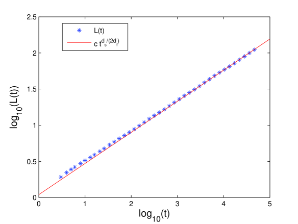
Figure 8: Growth of $L(t)$ as a function of time for the $O(4)$ model on the Sierpinski gasket, a comparison with the expected behaviour $ct^{d_{s}/(2d_{f})}$ is provided.

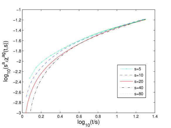
Figure 9: Scaling of the susceptibility $\chi^{ag}(t,s)$, for large $t/s$ a good agreement with the scaling hypothesis (17) with $a_{\chi}=d_{s}/2-1$ is evidenced.

5 Conclusions

In this paper, we have studied the phase-ordering kinetics of $O(3)$ and $O(4)$ models on self-similar physical graphs with known spectral dimension. On homogeneous lattices these models obey dynamical scaling. We have shown by means of extensive numerical simulations that the same symmetry appears to be obeyed also on the networks considered. The non-equilibrium exponents $z$ and $a_{\chi}$ are consistent with the value provided by the large-${\cal N}$ model. These results suggest that Equations (6) and (7) for $z$ and $a_{\chi}$ may hold for any ${\cal N}\geq 2$, for systems interested by dynamical scaling. It would important to substantiate this hypothesis by means of analytic calculations that go beyond the large-${\cal N}$ limit by accessing directly the case of finite ${\cal N}$. This could be possibly achieved by using a Gaussian Auxiliary Field approximation on the equation of motion for the $O({\cal N})$ model [21].

On the other hand, concerning the issue of the generality of the scaling property, it would be interesting to study if the breakdown of dynamical scaling always occurs in the $O(2)$ model on structures with $d_{s}<2$, similarly to what observed on homogeneous one-dimensional lattices [18].

Appendix A $O(2)$ model

In this appendix we present some results obtained for the $O(2)$ model using zero temperature heath bath dynamics (18). First we discuss phase ordering in a one-dimensional system. We show that our dynamics reproduce the asymptotic behaviour predicted analytically in [18] where zero-temperature phase ordering for the $O(2)$ model is studied by means of continuous time dissipative dynamics. In [18] it is evidenced that the dynamical scaling is violated since two different correlation lengths are present. The first one, the phase winding length $L(t)$, is the characteristic length of the spin spin-spin correlation function defined by Eq. (14). The other is the phase coherence length $L_{K}(t)$ representing the typical distance for which the winding of the spins along the system changes its direction. In particular, calling $-\pi<\theta_{i}<\pi$ the angle between neighbouring spins $\vec{\sigma}_{i}$ and $\vec{\sigma}_{i+1}$, one defines on each site the binary variable $k_{i}=\pm 1$ if $\theta_{i}>0$ or $\theta_{i}<0$ respectively. According to [18], the correlation function $G_{K}(r,t)=\langle k_{i}(t)k_{i+r}(t)\rangle$ scales differently from $G(r,t)$; in particular

$$G(r,t)=g(r/L(t))=g(x)~{}~{}~{}~{}G_{K}(r,t)=g_{k}(r/L_{K}(t))=g_{k}(x)$$ (19)

with $L(t)\sim t^{1/4}$ and $L_{K}(t)\sim t^{1/2}$. In our simulation with zero temperature heath bath dynamics we verify the laws (19). In particular in Fig. 10 we display the growth in time of the two correlation function evidencing a very good agreement with the expected results. We remark that adopting different dynamics, e.g. Metropolis, the analytically known behaviour is not easily reproduced in simulations because of very-long transients (only the asymptotic behaviour is expected to be independent of the transition rates).

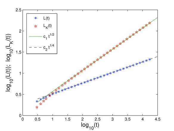
Figure 10: The growth of the correlation lengths $L(t)$ and $L_{K}(t)$.

As explained in Sec. 3 we have initially considered the $O(2)$ rotator model on fractals, and we obtain that the system gets frozen into metastable states. In particular the energy $E(t)$ does not tend to zero and the correlation length does not diverge. Figure 11 shows this behaviour for the Sierpinski gasket. Analogous behaviours are present on other fractals.

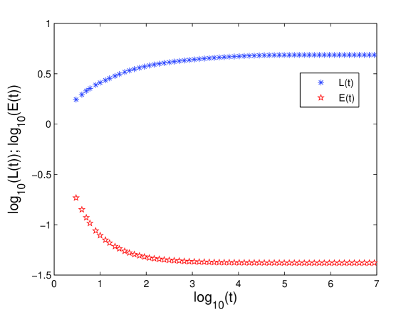
Figure 11: Correlation lengths $L(t)$ and energy $E(t)$ as a function of time in the $O(2)$ model on the Sierpinski gasket fractal. $L(t)$ is defined by Eq. 14. The energy scale is set so that the energy of the ground state is zero.

References

References

-
[1]
Furukawa H 1989 J.Stat.Soc.Jpn. 58, 216
Furukawa H 1989 Phys.Rev. B 40, 2341 - [2] Bouchaud J P, Cugliandolo L F , Kurchan J and Mézard M 1997 in Spin Glasses and Random Fields edited by A.P.Young (World Scientific, Singapore).
- [3] Bray A J, Adv.Phys. 43, 357
-
[4]
Corberi F, Lippiello E and Zannetti M 2003
Phys.Rev. E 68, 046131
Corberi F, Castellano C, Lippiello E and Zannetti M 2004 Phys.Rev. E 70 017103 - [5] Corberi F, Lippiello E and Zannetti M 2002 Phys. Rev. E 65 046136
-
[6]
Corberi F, Lippiello E and Zannetti M 2001
Phys. Rev. E 63 061506
Corberi F, Lippiello E and Zannetti M 2001 Eur. Phys.J. B 24, 359 -
[7]
Beysens D A, Forgacs G, Glazier J A 2000 Proc. Nat. Ac. Sci. 97, 9467
Castellano C, Marsili M, Vespignani A Phys. Rev. Lett. 85 3536 -
[8]
Burioni R, Cassi D and Vezzani A 2000 Eur. Phys. J. B 15 665
Burioni R and Cassi D 2005 Jour. Phys. A 38 R45 -
[9]
Alexander S and Orbach R 1982 J. Phys. Lett. 43 L62
Hattori K, Hattori T and Watanabe H 1987 Prog. Theor. Phys. Suppl. 92 108 -
[10]
Cassi D 1996 Phys. Rev. Lett. 76 2941
Burioni R, Cassi D and Vezzani A 1999 Phys. Rev. E 60 1500 - [11] Burioni R, Cassi D, and Destri C 2000 Phys. Rev. Lett. 85 1496
- [12] Marini Bettolo Marconi U and Petri A 1997 Phys. Rev. E 55, 1311
- [13] Burioni R, Cassi D, Corberi F and Vezzani A 2006 Phys. Rev. Lett. 96 235701
-
[14]
Gefen Y, Aharony A and Mandelbrot B B 1983 Jour. Phys. A 16 1267
Gefen Y, Aharony A, Shapir Y and Mandelbrot BB 1984 Jour. Phys. A 17 435 - [15] Rammal R 1984 J. Physique 45 191
- [16] Burioni R, Cassi D, Corberi F and Vezzani A 2007 Phys. Rev. E 75 011113
- [17] Grabner P J and Woess W, 1997 Stochastic Proc. Appl. 69 127 Bab M A, Fabricius G, and Albano E V 2005 Phys. Rev. E 71 036139
-
[18]
Newman T J, Bray A J and Moore M A 1990 Phys. Rev. B 42 4514
Rutenberg A D and Bray A J 1995 Phys. Rev. Lett. 74 3836 - [19] Cornell S J, Kaski K and Stinchcombe R B 1991 Phys. Rev. B 44 12263
- [20] Brown G, Rikvold P A, Sutton M, and Grant M 1997 Phys. Rev. E 56 6601
-
[21]
Mazenko G F 1990 Phys. Rev. B 42 4487
Mazenko G F 1991 Phys. Rev. B 43 5747
Yeung C, Oono Y and Shinozaki A, Phys. Rev. E 49 2693
De Siena S and Zannetti M 1984 Phys. Rev. E 50 2621