A QUANTUM GOLDMAN BRACKET FOR LOOPS ON SURFACES

Abstract

In the context of (2+1)–dimensional gravity, we use holonomies of constant connections which generate a $q$–deformed representation of the fundamental group to derive signed area phases which relate the quantum matrices assigned to homotopic loops. We use these features to determine a quantum Goldman bracket (commutator) for intersecting loops on surfaces, and discuss the resulting quantum geometry.

PACS numbers: 04.60.Kz, 02.20.Uw, Mathematics Subject Classification: 83C45

1 Introduction and background

There are many approaches to the quantization of gravity–without matter couplings–in 3 (2 space, 1 time) dimensions. We shall start with the Einstein action with nonzero cosmological constant

$$I_{\hbox{\scriptsize\it Ein}}=\int\!d^{3}x\sqrt{-{}^{\scriptscriptstyle(3)}\!g}\>({}^{\scriptscriptstyle(3)}\!R-2\Lambda).$$ (1.1)

In the first order-formalism (see Refs Achu–Witt and Refs NR0–NRZ) this action is written as

$$I_{\hbox{\scriptsize\it Ein}}=\int\-(d\omega^{ab}-{\omega^{a}}_{d}\wedge\omega^{db}+{\frac{\Lambda}{3}}e^{a}\wedge e^{b})\wedge e^{c}\,\epsilon_{abc},\qquad a,b,c=0,1,2.$$ (1.2)

where the triad $e^{a}$ is related to the metric through

$$g_{\mu\nu}={e^{a}}_{\mu}{e^{b}}_{\nu}\eta_{ab},$$ (1.3)

and the (2+1)-dimensional Ricci curvature and torsion are

$$R^{ab}=d\omega^{ab}-\omega^{ac}\wedge\omega_{c}{}^{b},\quad R^{a}=de^{a}-\omega^{ab}\wedge e_{b}$$ (1.4)

For $\Lambda\neq 0$, this action can be written (up to a total derivative) in the Chern-Simons form

$$I_{\hbox{\scriptsize CS}}=-\frac{\alpha}{4}\int(d\omega^{AB}-\frac{2}{3}\omega^{A}{}_{E}\wedge\omega^{EB})\wedge\omega^{CD}\epsilon_{ABCD},\qquad A,B,C,D=0,1,2,3$$ (1.5)

with an (anti-)de Sitter spin connection $\omega^{AB}$

$${\omega^{A}}_{B}=\left(\begin{array}[]{cc}\omega^{a}{}_{b}&\frac{ke^{a}}{\alpha}\\[4.30554pt] -\frac{e^{b}}{\alpha}&0\end{array}\right).$$ (1.6)

where the tangent space metric is $\eta_{AB}=(-1,1,1,k)$, and $k$ is the sign of $\Lambda$ with $\Lambda=k\alpha^{-2}$. In Eq. (1.5) the Levi-Civita density is $\epsilon_{abc3}=-\epsilon_{abc}$, and in (1.6) the triads appear as $e^{a}=\alpha\omega^{a3}$.

The corresponding curvature two-form $R^{AB}=d\omega^{AB}-\omega^{AC}\wedge\omega_{C}{}^{B}$ has components $R^{ab}+\Lambda e^{a}\wedge e^{b}$, $R^{a3}=\frac{R^{a}}{\alpha}$, and the field equations derived from the action (1.5) are simply $R^{AB}=0$, implying that the torsion vanishes everywhere and that the curvature $R^{ab}$ is constant. This can alternatively be seen from the (2+1)-dimensional splitting of spacetime, where the action (1.5) decomposes as

$$I_{\hbox{\scriptsize CS}}=\frac{\alpha}{4}\int\!dt\int\!d^{2}x\,\epsilon^{ij}\epsilon_{ABCD}\,(\omega^{CD}{}_{j}\,{\dot{\omega}}^{AB}{}_{i}-\omega^{AB}{}_{0}R^{CD}{}_{ij})$$ (1.7)

(with $\epsilon^{0ij}=-\epsilon^{ij}$), from which the constraints are

$$R^{AB}{}_{ij}=0.$$ (1.8)

The constraints (1.8) imply that the (anti-)de Sitter connection $\omega^{AB}{}_{i}$ is flat. It can therefore be written locally in terms of an $\hbox{SO}(3,1)$ ($\Lambda>0$) - or $\hbox{SO}(2,2)$ ($\Lambda<0$) - valued zero-form $\psi^{AB}$ as $d\psi^{AB}=\omega^{AC}\,\psi_{C}{}^{B}$. It is actually more convenient to use the spinor groups $\hbox{SL}(2,\mathbb{R})\otimes\hbox{SL}(2,\mathbb{R})$ (for $\hbox{SO}(2,2)$) and $\hbox{SL}(2,\mathbb{C})$ (for $\hbox{SO}(3,1)$). (Details of the spinor group decomposition can be found in Ref. NRZ.) Define the one-form

$$\Delta(x)=\Delta_{i}(x)dx^{i}=\frac{1}{4}\omega^{AB}(x)\gamma_{AB}$$ (1.9)

where $\gamma_{AB}=\frac{1}{2}\left[\gamma_{A},\gamma_{B}\right]$ and the $\gamma_{A}$ are Dirac matrices. Eq. (1.8) now implies that $d\Delta-\Delta\wedge\Delta=0$. The corresponding local or ”pure gauge” expression for $\Delta$ is

$$dS(x)=\Delta(x)S(x).$$ (1.10)

where $S$ are multivalued $\hbox{SL}(2,\mathbb{R})$ or $\hbox{SL}(2,\mathbb{C})$ matrices.

The above discussion means that the $\hbox{SO}(3,1)$ or $\hbox{SO}(2,2)$ - valued $\psi^{AB}$, or the $\hbox{SL}(2,\mathbb{R})$ or $\hbox{SL}(2,\mathbb{C})$ matrices $S$ can be interpreted as holonomies, when the connections $\omega^{AB}$ or $\Delta$ are integrated along closed paths (loops) on the two–dimensional surface $\Sigma$. The flatness of the connection $\Delta$ implies that each $S[\gamma]$ depends only on the homotopy class of $\gamma$. Further, the matrices $S$ are not gauge invariant, but are gauge covariant i.e. under a gauge transformation (a change of base point), they transform by conjugation.

The Einstein action can be used to gain further information about these holonomies. For example, the Poisson brackets of the $\omega^{AB}$ can be read off from (1.7): on a $t=\hbox{const.}$ surface $\Sigma$,

$$\{\omega^{AB}{}_{i}(x),\omega^{CD}{}_{j}(y)\}=\frac{k}{2\alpha}\epsilon_{ij}\epsilon^{ABCD}\delta^{2}(x-y).$$ (1.11)

and the spinor version is

$$\{\Delta_{i}^{\pm}(x),\Delta_{j}^{\pm}(y)\} = \pm\frac{i}{2\alpha\sqrt{k}}\epsilon_{ij}\sigma^{m}\otimes\sigma^{m}\delta^{2}(x-y)$$

$$\{\Delta_{i}^{+}(x),\Delta_{j}^{-}(y)\} = 0,$$ (1.12)

where the $\sigma^{m}$ are Pauli matrices, the $\pm$ refer to the decomposition of the $4\times 4$ representations of $\Delta(x)$, $S(x)$ into $2\times 2$ irreducible parts (see Ref. NRZ) and $\sqrt{k}$ means $+1$ for $k=1$ and $+i$ for $k=-1$.

The Poisson brackets Eqs. (1.11) and (1.12), when integrated along loops $\gamma,\sigma$ (with $\gamma,\sigma\!\in\!\pi_{1}(\Sigma,x_{0})$) yield the Poisson brackets of the components of the holonomies $\psi^{AB}$

$$\{{\psi^{AB}}_{\gamma},{\psi^{CD}}_{\sigma}\}=-k\epsilon^{ABCD}.$$ (1.13)

and a similar (complicated) expression for the $S^{\pm}$. The matrices $S^{\pm}[\gamma]$ thus furnish a representation of $\pi_{1}(\Sigma,x_{0})$ in $\hbox{SL}(2,\mathbb{R})$ or $\hbox{SL}(2,\mathbb{C})$. Under a gauge transformation the $S^{\pm}$ transform by conjugation, so their traces provide an (overcomplete) set of gauge-invariant Wilson loop variables.

The classical Poisson brackets for these trace variables were calculated by hand for the genus $1$ and genus $2$ cases, and then generalized and quantized in Ref. NR1. A closely related quantum algebra was calculated in Ref. ch using the technique of ”fat graphs”. The classical Poisson bracket algebra also appears (see Ref. ug) in the study of Stokes matrices (monodromy data) which relate the solutions of matrix differential equations. For genus 1 the Poisson algebra is

$$\{R_{1}^{\pm},R_{2}^{\pm}\}=\mp\frac{i}{4\alpha\sqrt{k}}(R_{12}^{\pm}-R_{1}^{\pm}R_{2}^{\pm})\quad\hbox{\it and cyclical permutations},$$ (1.14)

where $R^{\pm}=\frac{1}{2}\hbox{Tr}S^{\pm}$. Here the subscripts $1$ and $2$ refer to the two independent intersecting circumferences $\gamma_{1}$, $\gamma_{2}$ on $\Sigma$ with intersection number $+1$, while the third traced holonomy, $R^{\pm}_{12}$, corresponds to the path $\gamma_{1}\cdot\gamma_{2}$, which has intersection number $-1$ with $\gamma_{1}$ and $+1$ with $\gamma_{2}$.

Classically, the six traced holonomies $R^{\pm}_{1,2,12}$ provide an overcomplete description of the spacetime geometry of $\mathbb{R}\!\times\!T^{2}$. Consider the cubic polynomials

$$F^{\pm} = 1-(R_{1}^{\pm})^{2}-(R_{2}^{\pm})^{2}-(R_{12}^{\pm})^{2}+2R_{1}^{\pm}R_{2}^{\pm}R_{12}^{\pm}$$ (1.15)

$$= \frac{1}{2}\,\hbox{Tr}\left(I-S^{\pm}[\gamma_{1}]S^{\pm}[\gamma_{2}]S^{\pm}[\gamma_{1}^{-1}]S^{\pm}[\gamma_{2}^{-1}]\right),$$

where the last equality follows from the identities

$$A+A^{-1}=I\,\hbox{Tr}A$$

for $2\times 2$ matrices $A$ with determinant $1$. These polynomials have vanishing Poisson brackets with all of the traces $R_{a}^{\pm}$, and are cyclically symmetric in the $R_{a}^{\pm}$. The $F^{\pm}$ vanish classically by the $\hbox{SL}(2,\mathbb{R})$ or $\hbox{SL}(2,\mathbb{C})$ Mandelstam identities, which can be viewed as the application of the fundamental relation of $\pi_{1}$ of the torus

$$\gamma_{1}^{\vphantom{-1}}\cdot\gamma_{2}^{\vphantom{-1}}\cdot\gamma_{1}^{-1}\cdot\gamma_{2}^{-1}={\mathbb{I}}$$ (1.16)

to the representations $S^{\pm}$ occuring in the last line of (1.15).

In this approach, the constraints have been solved exactly. There is no Hamiltonian, and no time development. This formalism describes either initial data for some (unspecified) choice of time, or the time-independent spacetime geometry.

We can quantize the classical algebra (1.14) by firstly replacing the classical Poisson brackets $\{\,,\,\}$ with commutators $[\,,\,]$, with the rule

$$[x,y]=xy-yx=i\hbar\{x,y\};$$ (1.17)

and secondly, on the right hand side (r.h.s.) of (1.14), replacing the product with the symmetrized product,

$$xy\to\frac{1}{2}(xy+yx).$$ (1.18)

The resulting operator algebra is given by

$$\hat{R}_{1}^{\pm}\hat{R}_{2}^{\pm}e^{\pm i\theta}-\hat{R}_{2}^{\pm}\hat{R}_{1}^{\pm}e^{\mp i\theta}=\pm 2i\sin\theta\,\hat{R}_{12}^{\pm}\quad\hbox{\it and cyclical permutations}$$ (1.19)

with $\tan\theta={i\sqrt{k}\hbar}/{8\alpha}$. Note that for $\Lambda\!<\!0$, $k=-1$, and $\theta$ is real, while for $\Lambda\!>\!0$, $k=1$, and $\theta$ is pure imaginary.

The algebra (1.19) is not a Lie algebra, but it is related to the Lie algebra of the quantum group $\hbox{SU}(2)_{q}$ Refs. NRZ,su, where $q=\exp{4i\theta}$, and where the cyclically invariant $q$-Casimir is the quantum analog of the cubic polynomial (1.15),

$$\hat{F}^{\pm}(\theta)={\cos}^{2}\theta-e^{\pm 2i\theta}\left((\hat{R}_{1}^{\pm})^{2}+(\hat{R}_{12}^{\pm})^{2}\right)-e^{\mp 2i\theta}(\hat{R}_{2}^{\pm})^{2}+2e^{\pm i\theta}\cos\theta\hat{R}_{1}^{\pm}\hat{R}_{2}^{\pm}\hat{R}_{12}^{\pm}.$$ (1.20)

For $g>1$ it was shown in Ref. gav that the algebra calculated in Ref. NR1 is isomorphic to a non–standard deformation of $\hbox{SO}(2g+2)_{q}$.

The representations of the algebra (1.19) have been studied e.g. in Ref. NRZ. Here we choose to represent each $(\pm)$ copy of the $\hat{R}_{a}^{\pm}$ as

$$\hat{R}_{a}=\frac{1}{2}(\hat{A}_{a}+\hat{A}_{a}^{-1})$$ (1.21)

where, from (1.19) the $\hat{A}_{a}$ must satisfy (here we discuss the $(+)$ algebra, the $(-)$ algebra has $q^{-1}$ rather than $q$)

$$\hat{A}_{1}\hat{A}_{2}=q\hat{A}_{2}\hat{A}_{1}\quad\hbox{\it and cyclical permutations}$$ (1.22)

Relations of the type (1.22) are called quantum plane relations, or $q$–commutators, or Weyl pair relations. Returning to the untraced matrices $S$ one notes that, writing them in diagonal form as

$$S(\gamma_{i})=U_{i}=\left(\begin{array}[]{clcr}A_{i}&0\\ 0&A_{i}^{-1}\end{array}\right)\quad i=1,2$$ (1.23)

it follows that the (now quantum matrices) $\hat{U}_{1},\hat{U}_{2}$ must satisfy by both matrix and operator multiplication, the $q$–commutation relation

$$\hat{U}_{1}\hat{U}_{2}=q\hat{U}_{2}\hat{U}_{1}$$ (1.24)

i.e. they form a matrix–valued Weyl pair. Equation (1.24) can be understood as a deformation of Eq. (1.16).

The present authors decided to study the quantum matrices $\hat{U}_{1},\hat{U}_{2}$ which satisfy (1.24). Consider the diagonal representation

$$\hat{U}_{i}=\left(\begin{array}[]{clcr}e^{{\hat{r}_{i}}}&0\\ 0&e^{-{\hat{r}_{i}}}\end{array}\right)=e^{{\hat{r}_{i}}\sigma_{3}}\quad i=1,2$$ (1.25)

where $\sigma_{3}$ is a Pauli matrix. From the identity

$$e^{\hat{X}}e^{\hat{Y}}=e^{\hat{Y}}e^{\hat{X}}e^{[\hat{X},\hat{Y}]},$$ (1.26)

valid when $[\hat{X},\hat{Y}]$ is a $c$–number, it follows that the quantum parameters $\hat{r}_{1},\hat{r}_{2}$ (also used in Ref. cn) satisfy the commutator

$$[\hat{r}_{1},\hat{r}_{2}]=-\frac{i\hbar\sqrt{-\Lambda}}{4}.$$ (1.27)

We note that in order to make the connection with $2+1$–dimensional gravity it is necessary to consider both $\hbox{SL}(2,\mathbb{R})$ sectors. The mathematical properties of just one sector have been studied in Ref.NP3. In Section 2 a brief review of quantum matrices is given, whereas Section 3 discusses quantum holonomy matrices for homotopic paths, and shows how they are related by the signed area between the two paths. Section 4 uses these concepts to quantize a classical bracket due to Goldman (Ref. gol), thus obtaining commutators between intersecting loops on surfaces.

2 Quantum Matrix Pairs

Quantum matrix pairs - namely the quantum matrices $\hat{U}_{1},\hat{U}_{2}$ which satisfy (1.24) may, as mathematical objects, be thought of as a simultaneous generalization of two familiar notions of “quantum mathematics”, namely the quantum plane and quantum groups. Briefly, the quantum plane is described by two non-commuting coordinates $x$ and $y$ satisfying the relation

$$xy=qyx$$ (2.1)

whereas, for an example of a quantum group, consider the $2\times 2$ matrices of the form

$$U=\left(\begin{array}[]{cc}a&b\\ c&d\end{array}\right)$$ (2.2)

with non-commuting entries satisfying

$$ab=qba;\quad ac=qca;\quad ad-da=(q-q^{-1})bc;$$

$$bc=cb;\quad bd=qdb;\quad cd=qdc.$$ (2.3)

A good description of matrices of the type (2.2) whose entries satisfy (2.3) can be found in Ref. Vokos, but for our purposes maybe the most important property is that the matrix $U^{n}$ is another matrix of the same type with $q$ substituted by $q^{n}$.

These two concepts - the quantum plane and quantum groups - are not unrelated. Consider the column vector whose entries are the non-commuting coordinates $x$ and $y$. It can be checked that the components of the new column vector

$$\left(\begin{array}[]{c}{x^{\prime}}\\ {y^{\prime}}\end{array}\right)=U\left(\begin{array}[]{c}{x}\\ {y}\end{array}\right)$$ (2.4)

also satisfy

$$x^{\prime}y^{\prime}=qy^{\prime}x^{\prime}$$ (2.5)

Quantum matrices in both the diagonal and upper–triangular sectors satisfying the fundamental relation (1.24) have been studied in Refs. NP1,NP2. They combine the preservation of internal relations under multiplication, a quantum-group-like feature, with the fundamental $q$-commutation relation which holds between the two matrices. The non-trivial internal commutation relations arose in the following way: in the upper-triangular sector, it was found that trivial internal commutation relations for each matrix were not compatible with the fundamental relation (1.22), in that the resulting products no longer had commuting entries. However it was possible to determine patterns of non-trivial internal relations which are preserved under matrix multiplication.

For example, consider the pair of matrices satisfying (1.24)

$$U_{i}=\left(\begin{array}[]{cc}\alpha_{i}&\beta_{i}\\ 0&{\alpha_{i}}^{-1}\end{array}\right),\,\,\,\,i=1,2$$ (2.6)

It can be checked that, apart from the mutual relations

$$\alpha_{1}\alpha_{2}=q\alpha_{2}\alpha_{1},\quad\alpha_{1}\beta_{2}=q\beta_{2}{\alpha_{1}}^{-1},\quad\alpha_{2}\beta_{1}=q^{-1}\beta_{1}{\alpha_{2}}^{-1}.$$ (2.7)

which guarantee (1.24), the entries must also satisfy the following internal relations

$$\alpha_{i}\beta_{i}=\beta_{i}{\alpha_{i}}^{-1},\quad i=1,2.$$ (2.8)

In Ref. NP2 it was shown that indeed products of powers of these matrices have the same structure of internal relations, and also taking two different products gives rise to new quantum matrix pairs of the same type. However, the internal relations (2.8) differ in structure from the relations (2.3), and, moreover, do not simplify in the limit $q\rightarrow 1$, which distinguishes them from e.g. Majid’s braided matrices (see Ref. maj).

3 Homotopy and signed area

Consider quantum holonomy matrices simultaneously conjugated into diagonal form (conjugating both matrices by the same matrix $S\in SL(2,\mathbb{R})$ ) (see Eq. (1.25) which for convenience is repeated here)

$$\hat{U}_{i}=\left(\begin{array}[]{clcr}e^{{\hat{r}_{i}}}&0\\ 0&e^{-{\hat{r}_{i}}}\end{array}\right),\quad i=1,2.$$

where the $\hat{r}_{i},i=1,2$ satisfy (1.27). They can be thought of as arising from constant connections $\hat{A}$ as in Ref. mik

$$\hat{U}_{i}=\exp\int_{\gamma_{i}}\hat{A},\quad\hat{A}=(\hat{r}_{1}dx+\hat{r}_{2}dy)\left(\begin{array}[]{clcr}1&0\\ 0&-1\end{array}\right).$$ (3.1)

where $x,y$ are coordinates, with period 1, on the torus $T^{2}={\mathbb{R}^{2}}_{(x,y)}/\mathbb{Z}^{2}$, and $y$ is constant along $\gamma_{1}$ and $x$ is constant along $\gamma_{2}$.

We have investigated constant matrix–valued connections which generalize the connections (3.1), and applied them to a much larger class of loops, extending the assignments $\gamma_{1}\mapsto U_{1},\,\gamma_{2}\mapsto U_{2}$ by using the quantum connection (3.1) in the diagonal case. The larger class of loops are represented by piecewise linear (PL) paths between integer points in $\mathbb{R}^{2}$, using a representation of $T^{2}$ as $\mathbb{R}^{2}/\mathbb{Z}^{2}$. We show that the matrices for homotopic paths are related by a phase expressed in terms of the signed area between the paths. This leads to a definition of a $q$–deformed representation of the fundamental group where signed area phases relate the quantum matrices assigned to homotopic loops.

Consider piecewise-linear (PL) paths on the plane $\mathbb{R}^{2}$ starting at the origin $(0,0)$ and ending at an integer point $(m,n),\,m,n\in\mathbb{Z}$. Under the identification $T^{2}=\mathbb{R}^{2}/\mathbb{Z}^{2}$, these paths give rise to closed loops on $T^{2}$. The integers $m$ and $n$ are the winding numbers of the loop in the $\gamma_{1}$ and $\gamma_{2}$ directions respectively, and two loops on $T^{2}$ are homotopic to each other if and only if the corresponding paths in $\mathbb{R}^{2}$ end at the same point $(m,n)$

Suppose a PL path $p$ consists of $N$ straight segments $p_{1},\dots,p_{N}$. Any such segment $p_{i}$ may be translated to start at the origin and end at $(m,n)\in\mathbb{R}^{2}$ (here we use the fact that the connection $A$ is invariant under spatial translations). Then we assign to each segment $p_{i}$ the quantum matrix

$$U_{(m,n)}=\exp\int_{p_{i}}A=\exp\left((mr_{1}+nr_{2})\sigma_{3}\right)=\left(\begin{array}[]{cc}e^{mr_{1}+nr_{2}}&0\\ 0&e^{-mr_{1}-nr_{2}}\end{array}\right)$$ (3.2)

where $\sigma_{3}=\left(\begin{array}[]{clcr}1&0\\ 0&-1\end{array}\right)$, and to the path $p$ the product matrix

$$p\mapsto U_{p}:=\prod_{i=1}^{N}\exp\int_{p_{i}}A.$$ (3.3)

This assignment is obviously multiplicative under multiplication of paths, $(p,p^{\prime})\mapsto p\circ p^{\prime}$, which corresponds to translating $p^{\prime}$ to start at the endpoint of $p$ and concatenating.

Now consider the straight path from $(0,0)$ to $(m,n)$. For example, with $U_{1}=U_{(1,0)}$, $U_{2}=U_{(0,1)}$ these correctly obey the fundamental relation (1.24), which can be generalized to arbitrary straight paths, using Eq. (1.26).

$$U_{(m,n)}U_{(s,t)}=q^{mt-ns}U_{(s,t)}U_{(m,n)},$$ (3.4)

where $U_{(m,n)}$ is given by Eq. (3.2).

Equation (3.4) expresses the relation between the quantum matrices assigned to the two paths going from $(0,0)$ to $(m+s,n+t)$ in two different ways around the parallelogram generated by $(m,n)$ and $(s,t)$, It is also straightforward to show a triangle equation

$$U_{(m,n)}U_{(s,t)}=q^{(mt-ns)/2}U_{(m+s,n+t)},$$ (3.5)

which can be derived from the identity

$$e^{\hat{X}}e^{\hat{Y}}=e^{\hat{X}+\hat{Y}}e^{\frac{[\hat{X},\hat{Y}]}{2}},$$

which follows from (1.26).

Note that in both cases the exponent of $q$ relating the two homotopic paths is equal to the signed area between the path $p$ on the left hand side (l.h.s.) and the path $p^{\prime}$ on the r.h.s. i.e. equal to the area between $p$ and $p^{\prime}$, when the PL loop consisting of $p$ followed by the inverse of $p^{\prime}$ is oriented anticlockwise, and equal to minus the area between $p$ and $p^{\prime}$, when it is oriented clockwise. The signed area for the parallelogram is given by $\det\left(\begin{array}[]{cc}m&s\\ n&t\end{array}\right)=mt-ns$ and for the triangle by $\frac{1}{2}(mt-ns)$.

The discussion can be generalized to arbitrary non-self-intersecting PL paths $p$ and $p^{\prime}$ which connect $(0,0)$ to the same integer point $(m,n)$ in $\mathbb{R}^{2}$. These two paths may intersect each other several times, either transversally, or when they coincide along a shared segment. Together they bound a finite number of finite regions in the $xy$-plane. Now choose a triangulation of a compact region of $\mathbb{R}^{2}$ containing and compatible with the paths $p,\,p^{\prime}$, in the sense that each segment of the paths is made up of one or more edges of the triangulation. We take all the triangles in the triangulation to be positively oriented in the sense that their boundary is oriented anticlockwise in $\mathbb{R}^{2}$. Since $p$ and $p^{\prime}$ are homotopic, they are homologous, and because $H_{3}$ of the plane is trivial, there is a unique $2$-chain $c(p,p^{\prime})$ such that $\partial c(p,p^{\prime})=p-p^{\prime}$. Let this chain be given by

$$c(p,p^{\prime})=\sum_{\alpha\in R}n_{\alpha}t_{\alpha},$$ (3.6)

where $t_{\alpha}$ is a triangle of the triangulation indexed by $\alpha$ in the index set $R$, and $n_{\alpha}\ =\pm 1$ or $0$. Note that only triangles from the finite regions enclosed by $p$ and $p^{\prime}$ can belong to the support of the $2$-chain, and that the coefficient of any two triangles in the same finite region is the same.

The signed area between $p$ and $p^{\prime}$ is

$$S(p,p^{\prime})=\sum_{\alpha\in R}n_{\alpha}A(t_{\alpha}),$$ (3.7)

where $A(t_{\alpha})$ is the area of the triangle $t_{\alpha}$. This is clearly independent of the choice of triangulation of $\mathbb{R}^{2}$ compatible with $p,\,p^{\prime}$, since the sum of the areas of the triangles inside each enclosed region is the area of that region, whatever the triangulation. It follows that

$$U_{p}=q^{S(p,p^{\prime})}U_{p^{\prime}}.$$ (3.8)

4 Goldman bracket

There is a classical bracket due to Goldman Ref. gol for functions $T(\gamma)={\rm tr}\,U_{\gamma}$ defined on homotopy classes of loops $\gamma$, which for $U_{\gamma}\in SL(2,\mathbb{R})$ is:

$$\{T(\gamma_{1}),T(\gamma_{2})\}=\sum_{S\in\gamma_{1}\sharp\gamma_{2}}\epsilon(\gamma_{1},\gamma_{2},S)(T(\gamma_{1}S\gamma_{2})-T(\gamma_{1}S\gamma_{2}^{-1})).$$ (4.1)

Here $\gamma_{1}\sharp\gamma_{2}$ denotes the set of (transversal) intersection points of $\gamma_{1}$ and $\gamma_{2}$ and $\epsilon(\gamma_{1},\gamma_{2},S)$ is the intersection index for the intersection point $S$. $\gamma_{1}S\gamma_{2}$ and $\gamma_{1}S\gamma_{2}^{-1}$ denote loops which are rerouted at the intersection point $S$. In the following we show how Eq. (4.1) may be quantized using the concept of area phases for homotopic paths which was outlined in Section 3.

In order to study intersections of “straight” loops, represented in $\mathbb{R}^{2}$ by straight paths between $(0,0)$ and integer points $(m,n)$, consider their reduction to a fundamental domain of $\mathbb{R}^{2}$, namely the square with vertices $(0,0),(1,0),(1,1),(0,1)$.

Here are two examples of fundamental reduction. Figure 1 shows a path in the first quadrant, namely the path $(2,1)$, and its reduction to the fundamental domain

Figure 1: The path $(2,1)$ and its fundamental reduction

whereas in other quadrants fundamentally reduced paths start at other vertices (not $(0,0)$). For example in the second quadrant the path $(-1,2)$ will (in the fundamental domain) start at $(1,0)$ and end at $(0,1)$, as shown in Figure 2.

Figure 2: The path $(-1,2)$ and its fundamental reduction

When the path $(m,n)$ is a multiple of another integer path, we say it is reducible. Otherwise it is irreducible.

It should be clear that two paths intersect at points where their fundamental reductions intersect. We may only consider transversal intersections, namely when their respective tangent vectors are not collinear. For intersecting paths of multiplicity $1$, their intersection number at that point is $+1$ if the angle from the first tangent vector to the second is between $0$ and $180$ degrees, and $-1$ if between $180$ and $360$ degrees. For paths of multiplicity greater than $1$, the intersection number is multiplied by the multiplicities of the paths involved. Denote the intersection number between two paths $p_{1}$ and $p_{2}$ at $P$ (or $P,Q,R$ if more than one) by $\epsilon(p_{1},p_{2},P)$. The total intersection number for two paths is the sum of the intersection numbers for all the intersection points, denoted $\epsilon(p_{1},p_{2})$. Here are three simple (and not so simple) examples (in the fundamental domain) of single and multiple intersections.

1. If $p_{1}=(1,0)$ and $p_{2}=(0,1)$ there is a single intersection
   at $(0,0)$ with $\epsilon=+1$.

   

2. If $p_{1}=(2,1)$ and $p_{2}=(0,1)$ there are two intersections,
   at $P=(0,0)$ and $Q=(0,\frac{1}{2})$, each with $\epsilon=+1$. The total
   intersection number is $\epsilon=+2$

   

3. If $p_{1}=(1,2)$ and $p_{2}=(2,1)$ there are three intersections,
   at $P=(0,0)$, $Q=(\frac{2}{3},\frac{1}{3})$ and $R(\frac{1}{3},\frac{2}{3})$ (see figure), each with
   $\epsilon=-1$. The total intersection number is $\epsilon=-3$ (the point
   $S=(1,1)$ does not contribute since it coincides with the point $P$

   

It should be noted that

1. all intersections between a given pair of straight paths have the same sign, since in this representation their tangent vectors have constant direction along the loops.

2. the total intersection number between $p_{1}=(m,n)$ and $p_{2}=(s,t)$ is the determinant

   $$\epsilon(p_{1},p_{2})=\left|\begin{array}[]{clcr}m&n\\ s&t\end{array}\right|=mt-ns$$ (4.2)

   since the total intersection number is invariant under deformation, i.e. homotopy

   $$\epsilon((m,n),(s,t)) = \epsilon((m,0)+(0,n),(s,0)+(0,t))$$ (4.3)

   $$= \epsilon((m,0),(0,t))+\epsilon((0,n),(s,0))$$

   $$= mt-ns.$$

   Relation (4.2) is easily checked for the above examples.

Now consider two straight paths $p_{1}$ and $p_{2}$ intersecting at the point $P$. Their positive and negative reroutings are denoted $p_{1}Pp_{2}$ and $p_{1}Pp_{2}^{-1}$ respectively, where $p_{2}^{-1}=(-s,-t)$ if $p_{2}=(s,t)$. These reroutings are defined as follows: starting at the basepoint follow $p_{1}$ to $P$, continue on $p_{2}$ (or $p_{2}^{-1}$) back to $P$, then finish along $p_{1}$. Note that, in accordance with the above rule, if the intersection point $P$ is the basepoint itself, the reroutings $p_{1}Pp_{2}$ and $p_{1}Pp_{2}^{-1}$ start by following $p_{2}$ (or $p_{2}^{-1}$) from the basepoint back to itself, and then follow $p_{1}$ from the basepoint back to itself. Here we show the reroutings ($p_{1}Pp_{2}$ and $p_{1}Pp_{2}^{-1}$ respectively, and at the various intersection points $P,Q,R$ if more than one) for the three previous examples, using the non–reduced paths which here are more convenient.

1. $P=(0,0),p_{1}=(1,0),p_{2}=(0,1)$      

2. (a) $P=(0,0),p_{1}=(2,1),p_{2}=(0,1)$       (b) $Q=(0,\frac{1}{2}),p_{1}=(2,1),p_{2}=(0,1)$      

3. (a) $P=(0,0),p_{1}=(1,2),p_{2}=(2,1)$       (b) $Q=(\frac{2}{3},\frac{1}{3}),p_{1}=(1,2),p_{2}=(2,1)$       (c) $R=(\frac{1}{3},\frac{2}{3}),p_{1}=(1,2),p_{2}=(2,1)$      

In each of the above examples, and for each intersection point $P,Q,R$, it is clear that $p_{1}Pp_{2}\sim(m+s,n+t)$ and $p_{1}Pp_{2}^{-1}\sim(m-s,n-t)$.

To return to the bracket (4.1), we assign classical functions to the straight paths $(m,n)$ as follows

$$T(m,n)=e^{mr_{1}+nr_{2}}+e^{-mr_{1}-nr_{2}},$$ (4.4)

i.e. $T(m,n)={\rm tr}~{}~{}U_{(m,n)}$ where $U_{(m,n)}$ is of the form (3.2) with $r_{1},\,r_{2}$ classical parameters. Setting $\{r_{1},r_{2}\}=1$ it follows that the Poisson bracket between these functions for two paths $(m,n)$ and $(s,t)$ is

$$\{T(m,n),T(s,t)\}=(mt-ns)(T(m+s,n+t)-T(m-s,n-t))\{r_{1},r_{2}\}$$ (4.5)

Equation (4.5) may be regarded as a particular case of the Goldman bracket (4.1) (up to setting $\{r_{1},r_{2}\}=1$), since $(m,n)$ and $(s,t)$ have total intersection index $mt-ns$, and the rerouted paths $p_{1}Qp_{2}$ and $p_{1}Qp_{2}^{-1}$, where $p_{1}=(m,n)$ and $p_{2}=(s,t)$, are all homotopic to $(m+s,n+t)$ and $(m-s,n-t)$ respectively.

The bracket (4.5) is easily quantized using the triangle identity (see (3.5))

$$e^{mr_{1}+nr_{2}}e^{sr_{1}+tr_{2}}=q^{(mt-ns)/2}e^{(m+s)r_{1}+(n+t)r_{2}}$$ (4.6)

and the result is the commutator

$$[T(m,n),T(s,t)]=(q^{\frac{(mt-ns)}{2}}-q^{-\frac{(mt-ns)}{2}})(T(m+s,n+t)-T(m-s,n-t)).$$ (4.7)

The antisymmetry of (4.7) is evident (from (4.4) $T(m,n)=T(-m,-n)$). It can be checked that (4.7) satisfies the Jacobi identity, and that the classical limit, namely $q\to 1,\hbar\to 0$, of the commutator (4.7), given by

$$\{,\}=lim_{\hbar\to 0}\frac{[,]}{i\hbar}$$

is precisely (4.5).

Alternatively, there is a different version of equation (4.7) which treats each intersection point individually, and uses rerouted paths homotopic to “straight line” paths as discussed previously, since we have already seen in Section 3 that homotopic paths no longer have the same quantum matrix assigned to them, but only the same matrix up to a phase. Thus for an arbitrary PL path $p$ from $(0,0)$ to $(m,n)$, set

$$T(p)=q^{S(p,(m,n))}T(m,n).$$ (4.8)

The factor appearing in (4.8) is the same as that relating the quantum matrices $U_{p}$ and $U_{(m,n)}$, where $(m,n)$ is the straight path.

We will show how to rewrite (4.7) in terms of the rerouted paths for example 3, i.e. $p_{1}=(1,2),\,p_{2}=(2,1)$. From (4.7)

$$[T(1,2),T(2,1)]=(q^{-3/2}-q^{3/2})(T(3,3)-T(-1,1)).$$ (4.9)

The intersections occur at the points $P,R,Q$ (in that order, counting along $p_{1}$) as shown in Figure 3. For the positively rerouted paths we have

$$T((1,2)P(2,1)) = T((2,1)(1,2))=q^{3/2}T(3,3)$$ (4.10)

$$T((1,2)R(2,1)) = q^{-1}T((1,2)P(2,1))$$ (4.11)

$$T((1,2)Q(2,1)) = q^{-1}T((1,2)R(2,1))$$ (4.12)

and for the negative reroutings

$$T((1,2)P(-2,-1)) = T((-2,-1)(1,2))=q^{-3/2}T(-1,1)$$ (4.13)

$$T((1,2)R(-2,-1)) = qT((1,2)P(-2,-1))$$ (4.14)

$$T((1,2)Q(-2,-1)) = qT((1,2)R(-2,-1)).$$ (4.15)

The factors appearing in equations (4.11), (4.12), (4.14) and (4.15) (the reroutings at $R$ and $Q$) are shown in Figure 3, where it is clear that each large parallelogram is divided into three equal parallelograms, each of unit area. The factors in (4.10) and (4.13) (the reroutings at $P$) come from the triangle equation (3.5), and are shown in Figure 4, where the triangles have signed area $+\frac{3}{2}$ and $-\frac{3}{2}$ respectively.

Figure 3: The reroutings $(1,2)S(2,1)$ and $(1,2)S(-2,-1)$ for $S=P,R,Q$

Figure 4: Factors for the reroutings $(1,2)P(2,1)$ and $(1,2)P(-2,-1)$

Now equation (4.9) can be rewritten in the form:

$$[T(1,2),T(2,1)]=\sum_{S=P,R,Q}(q^{-1}-1)T((1,2)S(2,1))+(q-1)T((1,2)S(-2,-1)).$$ (4.16)

In the general case, for $p_{1}=(m,n)$ and $p_{2}=(s,t)$ with $mt-ns\neq 0$, we postulate that

$$[T(p_{1}),T(p_{2})]=\sum_{Q\in p_{1}\sharp p_{2}}(q^{\epsilon(p_{1},p_{2},Q)}-1)T(p_{1}Qp_{2})+(q^{-\epsilon(p_{1},p_{2},Q)}-1)T(p_{1}Qp_{2}^{-1})$$ (4.17)

quantizes the Goldman bracket (4.1).

We have proved equation (4.17) as follows: first assume that both $p_{1}$ and $p_{2}$ are irreducible, i.e. not multiples of other integer paths, and study the reroutings $p_{1}Qp_{2}$ at $Q$. They are paths similar to those of Figure 3, namely following $p_{1}$ to $Q$, then rerouting along a path parallel to $p_{2}$, then finishing along a path parallel to $p_{1}$. The reroutings along $p_{2}$ must clearly pass through an integer point inside the parallelogram formed by $p_{1}$ and $p_{2}$ (apart from when the intersection point is the origin). They also clearly pass through only one integer point since $p_{2}$ is irreducible. Consider two adjacent lines inside the parallelogram parallel to $p_{2}$ and passing through integer points. The area of each parallelogram between them is $1$. Consider for instance one of the middle parallelograms in Figure 3 (whose area we saw previously was $1$ as the three parallelograms are clearly of equal area and the area of the large parallelogram is $3$). This is the same area as that of a parallelogram with vertices at integer points, as can be shown, for example, by cutting it into two pieces along the line between (1,1) and (2,2), then regluing them together into a parallelogram with vertices at (1,1), (2,2), (3,2) and (4,3), as indicated in Figure 5. This latter area is equal to $1$ from Pick’s theorem [21] which states that the area $A(P)$ of a lattice polygon $P$ is

$$A(P)=I(P)+B(P)/2-1,$$ (4.18)

where $I(P)$ is the number of interior lattice points and $B(P)$ is the number of boundary points (for the parallelogram in the example $I(P)=0$ since the lines parallel to $p_{2}$ are adjacent, and $B(P)=4$ from the integer points at the four vertices, so $A(P)=0+4/2-1=1$.) Therefore in general the parallelogram determined by $p_{1}$ and $p_{2}$, whose total area is $A=|mt-ns|$, is divided up into $A$ smaller parallelograms of equal area by lines parallel to $p_{2}$ passing through the interior integer points of the parallelogram. The fact that the total area is equal to the number of internal integer points $+1$ is again a consequence of Pick’s theorem.

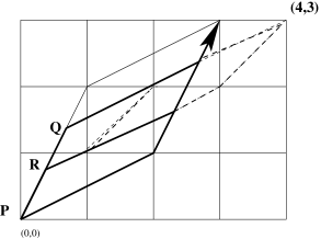
Figure 5: The area of the middle parallelogram is $1$

We can now calculate the first term (the positive reroutings shown for the example in Figure 3) in the sum on the r.h.s. of (4.17), using equation (4.8), and show that it is equal to the first term on the r.h.s. of (4.7). Consider first the case $\epsilon(p_{1},p_{2},Q)=-1$. The rerouting at the origin satisfies, using the triangle equation (3.5),

$$T(p_{1}\,(0,0)\,p_{2})=q^{A/2}T(m+s,n+t),$$

where the area of the parallelogram determined by $p_{1},\,p_{2}$ is $A=-(mt-ns)$. The next rerouted path adjacent to $p_{1}\,(0,0)\,p_{2}$, rerouted at $Q_{1}$ say (in the example $Q_{1}=R$) satisfies

$$T(p_{1}\,Q_{1}\,p_{2})=q^{-1}T(p_{1}\,(0,0)\,p_{2})$$

since we have shown that the signed area between the paths is $-1$. Similarly each successive adjacent path rerouted at $Q_{2},Q_{3},\dots$ satisfies

$$T(p_{1}\,Q_{i}\,p_{2})=q^{-1}T(p_{1}\,Q_{i-1}\,p_{2}).$$ (4.19)

with $Q_{0}$ the origin $(0,0)$. It follows that

$$\sum_{Q\in p_{1}\sharp p_{2}}(q^{-1}-1)T(p_{1}Qp_{2})$$ (4.20)

$$= (q^{-1}-1)q^{A/2}(1+q^{-1}+\dots+q^{-(A-1)})T(m+s,n+t)$$

$$= (q^{-1}-1)q^{A/2}\frac{1-q^{-A}}{1-q^{-1}}T(m+s,n+t)$$

$$= (q^{-A/2}-q^{A/2})T(m+s,n+t)$$

$$= (q^{(mt-ns)/2}-q^{-(mt-ns)/2})T(m+s,n+t).$$

When $\epsilon(p_{1},p_{2},Q)=+1$ the calculation is identical to (4.20) but with $q$ rather than $q^{-1}$, and with the area of the triangle now equal to $A/2$, where $A=mt-ns$, namely

$$\sum_{Q\in p_{1}\sharp p_{2}}(q-1)T(p_{1}\,Q\,p_{2})$$ (4.21)

$$= (q-1)q^{-A/2}(1+q^{1}+\dots+q^{A-1})T(m+s,n+t)$$

$$= (q^{A/2}-q^{-A/2})T(m+s,n+t)$$

$$= (q^{(mt-ns)/2}-q^{-(mt-ns)/2})T(m+s,n+t).$$

Diagrammatically this corresponds to dividing up the first parallelogram in Figure 3 by lines passing through the integer points in the interior, but parallel to $(1,2)$, as opposed to $(2,1)$.

In an entirely analogous way the second terms (the negative reroutings) on the r.h.s. of (4.7) and (4.17) can be shown to be equal - the second figure of Figure 3 can be used as a guide.

When $p_{1}$ is reducible, i.e. $p_{1}=c(m^{\prime},n^{\prime}),\,c\in\mathbb{N},m^{\prime},n^{\prime}\in\mathbb{Z}$, and $p_{2}$ is irreducible, formula (4.17) applies exactly as for the irreducible case, since there are $c$ times as many rerouted paths compared to the case when $p_{1}=(m^{\prime},n^{\prime})$. An example is $p_{1}=(2,0),\,p_{2}=(1,2)$, where the first term on the r.h.s. of (4.7) is equal to the first term on the r.h.s. of (4.17):

$$(q^{2}-q^{-2})T(3,2) = (q-1)q^{-2}(1+q+q^{2}+q^{3})T(3,2)$$ (4.22)

$$= \sum_{Q\in p_{1}\sharp p_{2}}(q-1)T(p_{1}Qp_{2}).$$

There are four rerouted paths in the final summation, rerouting at $(0,0)$, $(1/2,0)$, $(1,0)$ and $(3/2,0)$ along $p_{1}$.

If $p_{2}$ is reducible we must use multiple intersection numbers in (4.17), i.e. not simply $\pm 1$. Suppose $p_{1}=(m,n)$ and $p_{2}=(s,t)=c(s^{\prime},t^{\prime})$, $c\in\mathbb{N},s^{\prime},t^{\prime}\in\mathbb{Z}$. Then for example the first term on the r.h.s. of (4.17) with $mt-ns>0$ is

$$(q^{(mt-ns)/2}-q^{-(mt-ns)/2})T(m+s,n+t)$$ (4.23)

$$= (q^{c(mt^{\prime}-ns^{\prime})}-1)q^{-(mt-ns)/2}T(m+s,n+t)$$

$$= (q^{c}-1)q^{-(mt-ns)/2}(1+q^{c}+\dots+q^{c(mt^{\prime}-ns^{\prime}-1)})T(m+s,n+t)$$

$$= \sum_{Q\in p_{1}\sharp p_{2}}(q^{c}-1)T(p_{1}Qp_{2}).$$

The factor $(q^{c}-1)$ is the quantum multiple intersection number at the $mt^{\prime}-ns^{\prime}$ intersection points. The calculation can be regarded as doing equation (4.21) backwards and substituting $q$ by $q^{c}$ and $mt-ns$ by $mt^{\prime}-ns^{\prime}$. An example is $p_{1}=(2,1),\,p_{2}=(0,2)$, for which double intersections occur along $p_{1}$ at the origin and at $(1,1/2)$. From (4.23) the first term on the r.h.s. of (4.17) is

$$(q^{2}-q^{-2})T(2,3) = (q^{2}-1)q^{-2}(1+q^{2})T(2,3)$$ (4.24)

$$= (q^{2}-1)(T(p_{1}\,(0,0)\,p_{2})+T(p_{1}\,(1,1/2)\,p_{2}).$$

5 Conclusions

There are some surprising features of the quantum geometry that emerge from the use of a constant quantum connection. The phase factor appearing in the fundamental relation (1.24) has a geometrical origin as the signed area phase relating two integer PL paths, corresponding to two different loops on the torus. This leads to a natural concept of $q$-deformed surface group representations. It follows that the classical correspondence between flat connections (local geometry) and holonomies, i.e. group homomorphisms from $\pi_{1}$ to $G$ (non-local geometry) has a natural quantum counterpart.

The signed area phases also appear in a quantum version (4.17) of a classical bracket (4.1) due to Goldman Ref. gol, where classical intersection numbers $\pm\epsilon(p_{1},p_{2},Q)$ are replaced by quantum single and multiple intersection numbers $(q^{\pm\epsilon(p_{1},p_{2},Q)}-1)$.

The quantum bracket for homotopy classes represented by straight lines (4.7) is easily checked since all the reroutings are homotopic. However the r.h.s. of the bracket (4.17) may be expressed in terms of rerouted paths using the signed area phases and a far subtler picture emerges.

It is not difficult to show that the Jacobi identity holds for the commutator for straight paths (4.7) since the r.h.s. may also be expressed in terms of straight paths, with suitable phases. It must also hold for (4.17) since they are equivalent. We have checked it explicitly for a number of arbitrary PL paths, without identifying homotopic paths.

It should also be possible to treat higher genus surfaces (of genus $g$) in a similar fashion by introducing the same constant quantum connection on a domain in the $xy$ plane bounded by a $4g$–gon with the edges suitably identified [22]. One could then define holonomies of PL loops on this domain and study their behaviour under intersections, as studied here for $g=1$. In fact this treatment is ideal for $g>1$ since there intersections $\epsilon\geq 2$ are necessary (see e.g. Ref.  NR1).

References

• [1] A. Achúcarro and P. K. Townsend, Phys. Lett. B180, 89 (1986).
• [2] E. Witten, Nucl. Phys. B311, 46 (1988/89).
• [3] J. E. Nelson and T. Regge, Phys.Rev. D50, 5125 (1994).
• [4] J. E. Nelson and T. Regge, Phys. Lett. B272, 213 (1991).
• [5] J. E. Nelson and T. Regge, Nucl. Phys. B328, 190 (1989).
• [6] J. E. Nelson and T. Regge, Commun. Math. Phys. 141, 211 (1991).
• [7] J. E. Nelson and T. Regge, Commun. Math. Phys. 155, 561 (1993).
• [8] J. E. Nelson, T. Regge and F. Zertuche, Nucl. Phys. B339, 516 (1990).
• [9] L. O. Chekhov and V. V. Fock, Theor. Math. Phys. 120, 1245 (1999): Proc. Steklov Math. Inst. 226, 149 (1999).
• [10] M. Ugaglia, Int. Math. Res. Not. No. 9, 473 (1999).
• [11] M. Havlíček, A. V. Klimyk and S. Pošta J. Math. Phys. 40, 2135 (1999); D. B. Fairlie, J.Phys. A23, L183 (1990).
• [12] A. M. Gavrilik, in Proceedings of 3rd International Conference On Symmetry In Nonlinear Mathematical Physics, eds. A.G. Nikitin and V.M. Boyko, (Institute of Mathematics NAS of Ukraine, 2000).
• [13] S. Carlip and J. E. Nelson, Phys. Rev. D51, 5643 (1995).
• [14] J. E. Nelson and R. F. Picken, Phys. Lett. B471, 367 (2000).
• [15] J. E. Nelson and R. F. Picken, Lett. Math. Phys. 52, 277 (2000).
• [16] J. E. Nelson and R. F. Picken, Lett. Math. Phys. 59, 215 (2002).
• [17] W. M. Goldman, Invent. Math. 85, 263 (1986).
• [18] S. P. Vokos, B. Zumino and J. Wess, Z. Phys. C - Particles and Fields 48, 65 (1990).
• [19] S. Majid, Foundations of Quantum Group Theory, (Cambridge University Press, 1995).
• [20] A. Mikovic and R. F. Picken, Adv. Theor. Math. Phys. 5, 243 (2001).
• [21] G. Pick, Geometrisches zur Zahlentheorie Sitzenber. Lotos (Prague) 19, 311 (1899) and e.g. H.S.M. Coxeter, Introduction to Geometry, 2nd ed. (New York: Wiley) p. 209 (1969).
• [22] D. Hilbert and S. Cohn-Vossen, Geometry and the Imagination (transl. P. Nemenyi) (Chelsea Publishing Company, New York, 1990).