Missing values: sparse inverse covariance estimation and an extension to sparse regression

Abstract

We propose an $\ell_{1}$-regularized likelihood method for estimating the inverse covariance matrix in the high-dimensional multivariate normal model in presence of missing data. Our method is based on the assumption that the data are missing at random (MAR) which entails also the completely missing at random case. The implementation of the method is non-trivial as the observed negative log-likelihood generally is a complicated and non-convex function. We propose an efficient EM algorithm for optimization with provable numerical convergence properties. Furthermore, we extend the methodology to handle missing values in a sparse regression context. We demonstrate both methods on simulated and real data.
Keywords Gaussian graphical model, Lasso, Missing data, EM algorithm, Two-stage likelihood
This is the author’s version of the work (published in Statistics and Computing, 2012, Volume 22, 219-235). The final publication is available at www.springerlink.com.

1 Introduction

The most common probability model for continuous multivariate data is the multivariate normal distribution. Many standard methods for analyzing multivariate data, including factor analysis, principal components and discriminant analysis, are directly based on the sample mean and covariance matrix of the data.

Another important application are Gaussian graphical models where conditional dependencies among the variables are entailed in the inverse of the covariance matrix (Lauritzen, 1996). In particular, the inverse covariance matrix and its estimate should be sparse having some entries equaling zero since these encode conditional independencies. In the context of high-dimensional data where the number of variables $p$ is much larger than sample size $n$, Meinshausen and Bühlmann (2006) estimate a sparse Gaussian model by pursuing many $\ell_{1}$-penalized regressions for every node in the graph and they prove that the procedure can asymptotically recover the true graph. Later, other authors proposed algorithms for the exact optimization of the $\ell_{1}$-penalized log-likelihood (Yuan and Lin (2007), Friedman et al (2007b), Banerjee et al (2008) and Rothman et al (2008)). It has been shown in Ravikumar et al (2008) that such an approach is also able to recover asymptotically the true graph, but Meinshausen (2008) points out that rather restrictive conditions on the true covariance matrix are necessary. All these approaches and theoretical analyses have so far been developed for the case where all data is observed.

However, datasets often suffer from missing values (Little and Rubin, 1987). Besides many ad-hoc approaches to the missing-value problem, there is a systematic approach based on likelihoods which is very popular nowadays (Little and Rubin (1987), Schafer (1997)). But even estimation of mean values and covariance matrices becomes difficult when the data is incomplete and no explicit maximization of the likelihood is possible. A solution addressing this problem is given by the EM algorithm for solving missing-data problems based on likelihoods.

In this article we are interested in estimating the (inverse) covariance matrix and the mean vector in the high-dimensional multivariate normal model in presence of missing data, and this in turn allows for imputation. We present a new algorithm for maximizing the $\ell_{1}$-penalized observed log-likelihood. The proposed method can be used to estimate sparse undirected graphical models or/and regularized covariance matrices for high-dimensional data where $p\gg n$. Furthermore, once having a regularized covariance estimation for the incomplete data at hand, we show how to do $\ell_{1}$-penalized regression, when there is an additional response variable which is regressed on the incomplete data.

2 $\ell_{1}$-regularized inverse covariance estimation with missing data

2.1 GLasso

Let $(X^{(1)},\ldots,X^{(p)})$ be Gaussian distributed with mean $\mu$ and covariance $\Sigma$, i.e., $\mathcal{N}(\mu,\Sigma)$. We wish to estimate the concentration matrix $K=\Sigma^{-1}$. Given a complete random sample $\mathbf{x}=(x_{1},\ldots,x_{n})^{T}$, Yuan and Lin (2007) propose to minimize the negative $\ell_{1}$-penalized log-likelihood

$$-\ell(\mu,K;\mathbf{x})+\lambda\|K\|_{1}=-\frac{n}{2}\log|K|+\frac{1}{2}\sum_{i=1}^{n}(x_{i}-\mu)^{T}K(x_{i}-\mu)+\lambda\|K\|_{1},$$ (2.1)

over non-negative definite matrices $K$ ($K\succ 0$), where $\|K\|_{1}=\sum_{j,j^{\prime}=1}^{p}|K_{jj^{\prime}}|$. Here $\lambda>0$ is a tuning parameter.

The minimizer $\hat{K}$ is easily seen to satisfy

$$\hat{K} = \mathop{\arg\min}\limits_{K\succ 0}\big{(}-\log|K|+\mathrm{tr}(KS)+\rho\|K\|_{1}\big{)}$$ (2.2)

where $S=\frac{1}{n}\sum_{i=1}^{n}(x_{i}-\bar{x})(x_{i}-\bar{x})^{T}$ and $\rho=\frac{2\lambda}{n}$.

Friedman et al (2007b) propose an elegant and efficient algorithm, called GLasso, to solve the problem (2.2). We briefly review the derivation of their algorithm while details are given in Friedman et al (2007b) and Banerjee et al (2008). We will make use of this algorithm in the M-Step of an EM algorithm in a missing data setup, described in Section 2.3.2.

Using duality, formula (2.2) is seen to be equivalent to the maximization problem

$$\hat{\Sigma}=\mathop{\arg\max}\limits_{\|\Sigma-S\|_{\infty}\leq\rho}\log\det(\Sigma).$$ (2.3)

Problem (2.3) can be solved by a block coordinate descent optimization over each row and corresponding column of $\Sigma$. Partitioning $\Sigma$ and $S$

$$\Sigma=\left(\begin{array}[]{cc}\Sigma_{11}&\sigma_{12}\\ \sigma_{12}^{T}&\sigma_{22}\end{array}\right),\qquad S=\left(\begin{array}[]{cc}S_{11}&s_{12}\\ s_{12}^{T}&s_{22}\end{array}\right)$$

the block solution for the last column $\sigma_{12}$ satisfies

$$\hat{\sigma}_{12}=\mathop{\arg\min}\limits_{y:\|(y-s_{12})\|_{\infty}\leq\rho}y^{T}\Sigma_{11}^{-1}y.$$ (2.5)

Using duality it can be seen that solving (2.5) is equivalent to the Lasso problem

$$\hat{\beta}=\mathop{\arg\min}\limits_{\beta}\Big{(}\|\frac{1}{2}\Sigma_{11}^{1/2}\beta-\Sigma_{11}^{-1/2}s_{12}\|_{2}^{2}+\rho\|\beta\|_{1}\Big{)}$$ (2.6)

where $\hat{\sigma}_{12}$ and $\hat{\beta}$ are linked through $\hat{\sigma}_{12}=\Sigma_{11}\hat{\beta}/2$. Permuting rows and columns so that the target column is always the last, a Lasso problem like (2.6) is solved for each column, updating their estimate of $\Sigma$ after each stage. Fast coordinate descent algorithms for the Lasso (Friedman et al, 2007a) make this approach very attractive. Although the algorithm solves for $\Sigma$, the corresponding estimate of $K$ can be recovered cheaply.

2.2 MissGLasso

We turn now to the situation where some variables are missing (i.e., not observed).

As before, we assume $(X^{(1)},\ldots,X^{(p)})\sim\mathcal{N}(\mu,\Sigma)$ to be p-variate normally distributed with mean $\mu$ and covariance $\Sigma$. We then write $\mathbf{x}=(\mathbf{x}_{\mathrm{obs}},\mathbf{x}_{\mathrm{mis}})$, where $\mathbf{x}$ represents a random sample of size $n$, $\mathbf{x}_{\mathrm{obs}}$ denotes the set of observed values, and $\mathbf{x}_{\mathrm{mis}}$ the missing data. Also, let

$$\mathbf{x}_{\mathrm{obs}}=(x_{\mathrm{obs},1},x_{\mathrm{obs},2},\ldots,x_{\mathrm{obs},n}),$$

where $x_{\mathrm{obs},i}$ represents the set of variables observed for case $i$, $i=1,\ldots,n$.

A simple way to estimate the concentration matrix $K$ would be to delete all the cases which contain missing values and then estimating the covariance by solving the GLasso problem (2.2) using only the complete cases. However, excluding all cases having at least one missing variable can result in a substantial decrease of the sample size available for the analysis. When $p$ is large relative to $n$ this problem is even much more pronounced.

Another ad-hoc method would impute the missing values by the corresponding mean and then solving the GLasso problem. Such an approach is typically inferior to what we present below, see also Sections 4.1.1 and 4.1.4.

Much more promising is to base the inference for $\mu$ and $\Sigma$ (or $K$) in presence of missing values on the observed log-likelihood:

$$\ell(\mu,\Sigma;\mathbf{x}_{\mathrm{obs}})= \!-\frac{1}{2}\sum_{i=1}^{n}\Big{(}\log|\Sigma_{\mathrm{obs},i}|+(x_{\mathrm{obs},i}-\mu_{\mathrm{obs},i})^{T}(\Sigma_{\mathrm{obs},i})^{-1}(x_{\mathrm{obs},i}-\mu_{\mathrm{obs},i})\Big{)}$$ (2.7)

where $\mu_{\mathrm{obs},i}$ and $\Sigma_{\mathrm{obs},i}$ are the mean and covariance matrix of the observed components of $X$ (i.e., $X_{\mathrm{obs}}$) for observation $i$. Formally (2.7) can be re-written in terms of $K$

$$\ell(\mu,K;\mathbf{x}_{\mathrm{obs}})= \!-\!\frac{1}{2}\!\sum_{i=1}^{n}\!\Big{(}\!\!\log\!|(\!K^{-1})_{\mathrm{obs},i}|\!+\!(x_{\mathrm{obs},i}\!-\!\mu_{\mathrm{obs},i})^{T}\big{(}(K^{-1})_{\mathrm{obs},i}\big{)}^{-1}(x_{\mathrm{obs},i}-\mu_{\mathrm{obs},i})\Big{)}.$$ (2.8)

Inference for $\mu$ and $K$ can be based on the log-likelihood (2.8) if we assume that the underlying missing data mechanism is ignorable. The missing data mechanism is said to be ignorable if the probability that an observation is missing may depend on $\mathbf{x}_{\mathrm{obs}}$ but not on $\mathbf{x}_{\mathrm{mis}}$ (Missing at Random) and if the parameters of the data model and the parameters of the missingness mechanism are distinct. For a precise definition see Little and Rubin (1987).

Assuming that $p$ is large relative to $n$, we propose for the unknown parameters $(\mu,K)$ the estimator:

$$\hat{\mu},\hat{K} = \mathop{\arg\min}\limits_{(\mu,K):K\succ 0}-\ell_{\mathrm{pen}}(\mu,K;\mathbf{x}_{\mathrm{obs}})$$ (2.9)

$$-\ell_{\mathrm{pen}}(\mu,K;\mathbf{x}_{\mathrm{obs}}) = -\ell(\mu,K;\mathbf{x}_{\mathrm{obs}})+\lambda\|K\|_{1}$$ (2.10)

where $\ell(\mu,K;\mathbf{x}_{\mathrm{obs}})$ is given in (2.8). We call this estimator the MissGLasso.

Despite the concise appearance of (2.8), the observed log-likelihood tends to be a complicated (non-convex) function of the individual $\mu_{j}$ and $K_{jj^{\prime}}$, $j,j^{\prime}=1,\ldots,p$, for a general missing data pattern, with possible existence of multiple stationary points (Murray (1977); Schafer (1997)). Optimization of (2.9) is a non-trivial issue. An efficient algorithm is presented in the next section.

2.3 Computation

For the derivation of our algorithm presented in Section 2.3.2 we will state first some facts about the conditional distribution of the Multivariate Normal (MVN) Model.

2.3.1 Conditional distribution of the MVN Model and conditional mean imputation

Consider a partition $(X_{1},X_{2})\sim\mathcal{N}(\mu,\Sigma)$. It is well known that $X_{2}|X_{1}$ follows a linear regression on $X_{1}$ with mean $\mu_{2}+\Sigma_{21}\Sigma_{11}^{-1}(X_{1}-\mu_{1})$ and covariance $\Sigma_{22}-\Sigma_{21}\Sigma_{11}^{-1}\Sigma_{12}$ (Lauritzen, 1996). Thus,

$$X_{2}|X_{1}\!\sim\mathcal{N}\big{(}\mu_{2}\!+\!\Sigma_{21}\Sigma_{11}^{-1}\!(X_{1}-\mu_{1}),\Sigma_{22}\!-\!\Sigma_{21}\Sigma_{11}^{-1}\Sigma_{12}\big{)}.$$ (2.11)

Expanding the identity $K\Sigma=I$ gives the following useful expression:

$$\left(\begin{array}[]{cc}K_{11}&K_{12}\\ K_{21}&K_{22}\end{array}\right)\left(\begin{array}[]{cc}\Sigma_{11}&\Sigma_{12}\\ \Sigma_{21}&\Sigma_{22}\end{array}\right) = \left(\begin{array}[]{cc}I&0\\ 0&I\end{array}\right).$$ (2.18)

Using (2.18) we can re-express (2.11) in terms of $K$:

$$X_{2}|X_{1}\sim\mathcal{N}\big{(}\mu_{2}-K_{22}^{-1}K_{21}(X_{1}-\mu_{1}),K_{22}^{-1}\big{)}.$$ (2.19)

Formula (2.19) will be used later in our developed EM algorithm for estimation of the mean $\mu$ and the concentration matrix $K$ based on a random sample with missing values.

The spirit of this EM algorithm, see Section 2.3.2, is captured by the following method of imputing missing values by conditional means due to Buck (1960):

• Estimate $(\mu,K)$ by solving the GLasso problem (2.2) using only the complete cases (delete the rows with missing values). This gives estimates $\hat{\mu}$, $\hat{K}$.

• Use these estimates to calculate the least squares linear regressions of the missing variables on the present variables, case by case: From the above discussion about the multivariate normal distribution, the missing variables of case $i$, $x_{\mathrm{mis},i}$, given $x_{\mathrm{obs},i}$ are normally distributed with mean

  $$\mathbb{E}[x_{\mathrm{mis},i}|x_{\mathrm{obs},i},\mu,K]= \mu_{\mathrm{mis}}-(K_{\mathrm{mis},\mathrm{mis}})^{-1}K_{\mathrm{mis},\mathrm{obs}}\left(x_{\mathrm{obs},i}-\mu_{\mathrm{obs}}\right).$$

  Therefore an imputation of the missing values can be done by

  $$\hat{x}_{\mathrm{mis},i}:=\hat{\mu}_{\mathrm{mis}}-(\hat{K}_{\mathrm{mis},\mathrm{mis}})^{-1}\hat{K}_{\mathrm{mis},\mathrm{obs}}\left(x_{\mathrm{obs},i}-\hat{\mu}_{\mathrm{obs}}\right).$$

  Here, $\hat{\mu}_{\mathrm{obs}}$ and $\hat{\mu}_{\mathrm{mis}}$ depend on case $i$. Furthermore, $\hat{K}_{\mathrm{mis},\mathrm{mis}}$ denotes the sub-matrix of $\hat{K}$ with rows and columns corresponding to the missing variables for case $i$. Similarly $\hat{K}_{\mathrm{mis},\mathrm{obs}}$ denotes the sub-matrix with rows corresponding to the missing variables and columns corresponding to the observed variables for case $i$. Note that we always notationally suppress the dependence on $i$.

• Finally, re-estimate $(\mu,K)$ by solving the GLasso problem on the completed data in step 2.

2.3.2 $\ell_{1}$-norm penalized likelihood estimation via the EM algorithm

A convenient method for optimizing incomplete data problems like (2.9) is the EM algorithm (Dempster et al (1977)).

To derive the EM algorithm for minimizing (2.9) we note that the complete data follows a multivariate normal distribution, which belongs to the regular exponential family with sufficient statistics

$$\mathbf{T}_{1}=\mathbf{x}^{T}1=\left(\sum_{i=1}^{n}x_{i1},\sum_{i=1}^{n}x_{i2},\ldots,\sum_{i=1}^{n}x_{ip}\right)$$

and

$$\mathbf{T}_{2} =\mathbf{x}^{T}\mathbf{x}=\left(\begin{array}[]{cccc}\sum_{i=1}^{n}x_{i1}^{2}&\sum_{i=1}^{n}x_{i1}x_{i2}&\ldots&\sum_{i=1}^{n}x_{i1}x_{ip}\\ \sum_{i=1}^{n}x_{i2}x_{i1}&\sum_{i=1}^{n}x_{i2}^{2}&\ldots&\sum_{i=1}^{n}x_{i2}x_{ip}\\ \vdots&\vdots&&\vdots\\ \sum_{i=1}^{n}x_{ip}x_{i1}&\sum_{i=1}^{n}x_{ip}x_{i2}&\ldots&\sum_{i=1}^{n}x_{ip}^{2}\\ \end{array}\right).$$

The complete penalized negative log-likelihood (2.1) can be expressed in term of the sufficient statistics $\mathbf{T}_{1}$ and $\mathbf{T}_{2}$:

$$-\ell(\mu,K;\mathbf{x})+\!\lambda\|K\|_{1}= \!-\frac{n}{2}\!\log\!|K|\!+\frac{n}{2}\mu^{T}K\mu-\!\mu^{T}K\mathbf{T}_{1}+\frac{1}{2}\mathrm{tr}(K\mathbf{T}_{2})+\lambda\|K\|_{1}$$ (2.20)

which is linear in $\mathbf{T}_{1}$ and $\mathbf{T}_{2}$. The expected complete penalized log-likelihood is denoted by:

$$\mathop{Q}(\mu,K|\mu^{\prime},K^{\prime})=-\mathbb{E}[\ell(\mu,K;\mathbf{x})|\mathbf{x}_{\mathrm{obs}},\mu^{\prime},K^{\prime}]+\lambda\|K\|_{1}.$$

The EM algorithm works by iterating between the E- and M-Step. Denote the parameter value at iteration $m$ by $(\mu^{(m)},K^{(m)})$ (m=0,1,2,…), where $(\mu^{(0)},K^{(0)})$ are the starting values.

E-Step: Compute $\mathop{Q}(\mu,K|\mu^{(m)},K^{(m)})$:

As the complete penalized negative log-likelihood in (2.20) is linear in $\mathbf{T}_{1}$ and $\mathbf{T}_{2}$, the E-Step consists of calculating:

$$\mathbf{T}_{1}^{(m+1)}=\mathbb{E}[\mathbf{T}_{1}|\mathbf{x}_{\mathrm{obs}},\mu^{(m)},K^{(m)}]\quad\textrm{and}\quad\mathbf{T}_{2}^{(m+1)}=\mathbb{E}[\mathbf{T}_{2}|\mathbf{x}_{\mathrm{obs}},\mu^{(m)},K^{(m)}].$$

This involves computation of the conditional expectation of $x_{ij}$ and $x_{ij}x_{ij^{\prime}}$, $i=1,\ldots,n,\;j,j^{\prime}=1,\ldots,p$. Using formula (2.19) we find

$$\mathbb{E}[x_{ij}|x_{\mathrm{obs},i},\mu^{(m)},K^{(m)}]=\left\{\begin{array}[]{ll}x_{ij}&\textrm{if $x_{ij}$ observed}\\ c_{j}&\textrm{if $x_{ij}$ missing}\end{array}\right.$$

where $c$ is defined as

$$c:=\mu^{(m)}_{\mathrm{mis}}-(K^{(m)}_{\mathrm{mis},\mathrm{mis}})^{-1}K^{(m)}_{\mathrm{mis},\mathrm{obs}}\big{(}x_{\mathrm{obs},i}-\mu^{(m)}_{\mathrm{obs}}\big{)}.$$

Similarly, we compute

$$\mathbb{E}[x_{ij}x_{ij^{\prime}}|x_{\mathrm{obs},i},\mu^{(m)},K^{(m)}]=\left\{\begin{array}[]{ll}x_{ij}x_{ij^{\prime}}&\textrm{if $x_{ij}$ \& $x_{ij^{\prime}}$ observed,}\\ x_{ij}c_{j^{\prime}}&\textrm{if $x_{ij}$ observed, $x_{ij^{\prime}}$ missing,}\\ \big{(}K_{\mathrm{mis},\mathrm{mis}}^{(m)}\big{)}^{-1}_{jj^{\prime}}+c_{j}c_{j^{\prime}}&\textrm{if $x_{ij}$ \& $x_{ij^{\prime}}$ missing.}\\ \end{array}\right.$$

Here the vector $c$ and the matrix $\big{(}K_{\mathrm{mis},\mathrm{mis}}^{(m)}\big{)}^{-1}$ are regarded as naturally embedded in $\mathbb{R}^{p}$ and $\mathbb{R}^{p\times p}$ respectively, such that the obvious indexing makes sense.

The E-Step involves inversion of a sparse matrix, namely $K^{(m)}_{\mathrm{mis},\mathrm{mis}}$, for which we can use sparse linear algebra. Note also that $K^{(m)}_{\mathrm{mis},\mathrm{mis}}$ is positive definite and therefore invertible. Furthermore, considerable savings in computation are obtained if cases with the same pattern of missing $X$’s are grouped together.

M-Step: Compute the updates $(\mu^{(m+1)},K^{(m+1)})$ as minimizer of $\mathop{Q}(\mu,K|\mu^{(m)},K^{(m)})$:

It is easily seen from Equation (2.20) that $\mu^{(m+1)}$ and $K^{(m+1)}$ fulfill the following equations:

$$\mu^{(m+1)}=\frac{1}{n}\mathbf{T}_{1}^{(m+1)}$$

$$K^{(m+1)}=\mathop{\arg\min}\limits_{K\succ 0}\Big{(}-\log|K|+\mathrm{tr}(K\mathbf{S}^{(m+1)})+\frac{2\lambda}{n}\|K\|_{1}\Big{)}$$

where $\mathbf{S}^{(m+1)}=\frac{1}{n}\mathbf{T}_{2}^{(m+1)}-\mu^{(m+1)}(\mu^{(m+1)})^{T}$. Therefore the M-Step reduces to a GLasso problem of the form (2.2), which can be solved by the algorithm described in Section 2.1.

2.3.3 Numerical properties

A nice property of every EM algorithm is that the objective function is reduced in each iteration,

$$-\ell_{\mathrm{pen}}(\mu^{(m+1)},K^{(m+1)};\mathbf{x}_{\mathrm{obs}})\leq-\ell_{\mathrm{pen}}(\mu^{(m)},K^{(m)};\mathbf{x}_{\mathrm{obs}}).$$

Nevertheless the descent property does not guarantee convergence to a stationary point.

A detailed account of the convergence properties of the EM algorithm in a general setting has been given by Wu (1983). Under mild regularity conditions including differentiability and continuity, convergence to stationary points is proven for the EM algorithm.

For the EM algorithm described in Section 2.3.2 which optimizes a non-differentiable function we have the following result:

Proposition 2.1.

Every limit point $(\bar{\mu},\bar{K})$, with $\bar{K}\succ 0$, of the sequence $\{(\mu^{(m)},K^{(m)});m=0,1,2,\ldots\}$, generated by the EM algorithm, is a stationary point of the criterion function in (2.10).

A proof is given in the Appendix.

2.3.4 Selection of the tuning parameter

In practice a tuning parameter $\lambda$ has to be chosen in order to tradeoff goodness-of-fit and model complexity. One possibility is to use a modified BIC criterion which minimizes

$$\textrm{BIC}=-2\ell(\hat{\mu},\hat{K};\mathbf{x}_{\mathrm{obs}})+\log(n)\textrm{df},$$

over a grid of candidate values for $\lambda$. Here $(\hat{\mu},\hat{K})$ denotes the MissGLasso estimator (2.9) using the tuning parameter $\lambda$ and $\textrm{df}=\sum_{j\leq j^{\prime}}1_{\{\hat{K}_{jj^{\prime}}\neq 0\}}$ are the degrees of freedom (Yuan and Lin, 2007). The defined BIC criterion is based on the observed log-likelihood $\ell(\mu,K;\mathbf{x}_{\mathrm{obs}})$ which is also suggested by Ibrahim et al (2008).

Another possibility to tune $\lambda$ is to use the popular V-fold cross-validation method, based on the observed negative log-likelihood as loss function. We proceed as follows: First divide all the samples into V disjoint subgroups (folds), and denote the samples in $v$th fold by $N_{v}$ for $v=1,\ldots,V$. The V-fold cross-validation score is defined as:

$$CV(\lambda)= \sum_{v=1}^{V}\!\bigg{(}\!\sum_{i\in N_{v}}\!\!\log\!|(\hat{\Sigma}_{-v})_{\mathrm{obs},i}|+(x_{\mathrm{obs},i}\!-(\hat{\mu}_{-v}\!)_{\mathrm{obs},i})^{T}((\!\hat{\Sigma}_{-v})_{\mathrm{obs},i})^{-1}(x_{\mathrm{obs},i}-(\hat{\mu}_{-v})_{\mathrm{obs},i})\bigg{)}$$

where $\hat{\Sigma}_{-v}=(\hat{K}_{-v})^{-1}$, $\hat{K}_{-v}$ and $\hat{\mu}_{-v}$ denote the estimates based on the sample $(\cup_{v^{\prime}=1}^{V}N_{v^{\prime}})/N_{v}$. Then, find the best $\hat{\lambda}$ that minimizes $CV(\lambda)$. Finally, fit the MissGLasso to all the data using $\hat{\lambda}$ to get the final estimator of the inverse covariance matrix.

3 Extension to sparse regression

The MissGLasso could be applied directly to high-dimensional regression with missing values. Suppose a scalar response variable $Y$ is regressed on $p$ predictor variables $X^{(1)},\ldots,X^{(p)}$. If we assume joint multivariate normality for $\widetilde{X}=(Y,X^{(1)},\ldots,X^{(p)})$ with mean and concentration matrix given by

$$\tilde{\mu}=(\tilde{\mu}_{y},\tilde{\mu}_{x}),\qquad\widetilde{K}=\left(\begin{array}[]{cc}\tilde{k}_{yy}&\tilde{k}_{yx}\\ \tilde{k}_{yx}^{T}&\widetilde{K}_{xx}\end{array}\right),$$

we can estimate $(\tilde{\mu},\widetilde{K})$ with the MissGLasso. The regression coefficients $\hat{\beta}$ are then given by $\hat{\beta}=-\hat{\tilde{k}}_{yy}^{-1}\hat{\tilde{k}}_{yx}$. This approach is short-sighted: a zero in the concentration matrix, say ${\widetilde{K}}_{jj^{\prime}}=0$, means that $\widetilde{X}^{(j)}$ and $\widetilde{X}^{(j^{\prime})}$ are conditionally independent given all other variables in $\widetilde{X}$, where $Y$ is included in $\widetilde{X}$. But we typically care about conditional independence of $X^{(j)}$ and $X^{(j^{\prime})}$ given all other variables in $X$ (which does not include $Y$). In other words, we think that sparsity in the concentration matrix $K$ of $X$ (and of course $\beta$) is desirable. However, sparsity in the matrix $K$ is not enforced by penalizing $\|\widetilde{K}\|_{1}$. This can be seen by noting that $\widehat{K}=\big{(}\widehat{\widetilde{\Sigma}}_{xx}\big{)}^{-1}$ is not sparse for most cases of sparse estimates $\widehat{\widetilde{K}}$. For a similar discussion about this issue, see Witten and Tibshirani (2009).

We describe in Section 3.2 a two-stage procedure which results in sparse estimates for the concentration matrix $K$ of $X$ and the regression parameters $\beta$. In order to motivate the second stage of this procedure, we first introduce a likelihood-based method for sparse regression with complete data.

3.1 $\ell_{1}$-penalization in the regression model with complete data

Consider a Gaussian linear model:

$$Y_{i}=\beta^{T}X_{i}+\epsilon_{i},\quad i=1,\ldots,n,$$

$$\epsilon_{1},\ldots,\epsilon_{n}\quad\textrm{i.i.d.}\sim\mathcal{N}(0,\sigma^{2}),$$

where $X_{i}\in\mathbb{R}^{p}$ are covariates.

In the usual linear regression model, the $\ell_{1}$-norm penalized estimator, called the Lasso (Tibshirani (1996)), is defined as:

$$\hat{\beta}_{\lambda} = \mathop{\arg\min}\limits_{\beta}\frac{1}{2}\|\mathbf{y}-\mathbf{x}\beta\|^{2}+\lambda\|\beta\|_{1},$$ (3.22)

with $n\times 1$ vector $\mathbf{y}$, $p\times 1$ regression vector $\beta$ and $n\times p$ design matrix $\mathbf{x}$. The Lasso estimator in (3.22) is not likelihood-based and does not provide an estimate of the nuisance parameter $\sigma$. In Städler et al (2010), we suggest to take $\sigma$ into the definition and optimization of a penalized likelihood estimator: we proceed with the following estimator,

$$\hat{\beta}_{\lambda},\hat{\sigma}_{\lambda}= \mathop{\arg\min}\limits_{\beta,\sigma}-\ell(\beta,\sigma;\mathbf{y}|\mathbf{x})+\lambda\frac{\|\beta\|_{1}}{\sigma}$$

$$= \mathop{\arg\min}\limits_{\beta,\sigma}\Big{(}n\log(\sigma)\!+\frac{1}{2\sigma^{2}}\!\|\mathbf{y}-\!\mathbf{x}\beta\|^{2}\!+\lambda\frac{\|\beta\|_{1}}{\sigma}\Big{)}.$$ (3.23)

Intuitively the estimator (3.1) penalizes the $\ell_{1}$-norm of the regression coefficients and small variances $\sigma$ simultaneously. Furthermore this estimator is equivariant under scaling (see Städler et al (2010)). Most importantly if we reparametrize $\rho=1/\sigma$ and $\phi=\beta/\sigma$ we get the following convex optimization problem:

$$\hat{\phi}_{\lambda},\hat{\rho}_{\lambda}= \mathop{\arg\min}\limits_{\phi,\rho}\Big{(}\!-n\log(\rho)+\!\frac{1}{2}\!\|\rho\mathbf{y}-\!\mathbf{x}\phi\|^{2}+\!\lambda\|\phi\|_{1}\Big{)}.$$ (3.24)

This optimization problem can be solved efficiently in a coordinate-wise fashion. The following algorithm is very easy to implement, it simply updates, in each iteration, $\rho$ followed by the coordinates $\phi_{j}$, $j=1,\ldots,p$, of $\phi$.

Coordinate-wise algorithm for solving (3.24)

• Start with initial guesses for $\phi^{(0)},\rho^{(0)}$.

• Update the current estimates $\phi^{(m)},\rho^{(m)}$ coordinate-wise by:

  $$\rho^{(m+1)} = \frac{\mathbf{y}^{T}\mathbf{x}\phi^{(m)}+\sqrt{(\mathbf{y}^{T}\mathbf{x}\phi^{(m)})^{2}+4\mathbf{y}^{T}\mathbf{y}n}}{2\mathbf{y}^{T}\mathbf{y}}$$

  $$\phi_{j}^{(m+1)} = \left\{\begin{array}[]{ll}0&\textrm{if $|S_{j}|\leq\lambda$}\\ (\lambda-S_{j})/\mathbf{x}_{j}^{T}\mathbf{x}_{j}&\textrm{if $S_{j}>\lambda$}\\ -(\lambda+S_{j})/\mathbf{x}_{j}^{T}\mathbf{x}_{j}&\textrm{if $S_{j}<-\lambda$}\end{array}\right.$$

  where $S_{j}$ is defined as

  $$S_{j}=-\rho^{(m+1)}\mathbf{x}_{j}^{T}\mathbf{y}+\sum\limits_{s<j}\phi_{s}^{(m+1)}\mathbf{x}_{j}^{T}\mathbf{x}_{s}+\sum\limits_{s>j}\phi_{s}^{(m)}\mathbf{x}_{j}^{T}\mathbf{x}_{s}$$

  and $j=1,\ldots,p$.

• Iterate step 2 until convergence.

With $\mathbf{x}_{j}$ we denote the $j$th column vector of the $n\times p$ matrix $\mathbf{x}$. This algorithm can be implemented very efficiently as it is the case for the coordinate descent algorithm solving the usual Lasso problem. For example naive updates, covariance updates and the active-set strategy described in Friedman et al (2007a) and Friedman et al (2010) are applicable here as well.

Numerical convergence of the above algorithm is ensured as follows.

Proposition 3.1.

Every limit point $(\bar{\rho},\bar{\phi})$ of the sequence $\{(\rho^{(m)},\phi^{(m)});m=0,1,2,\ldots\}$, generated by the above algorithm, is a stationary point of the criterion function in (3.24).

A proof is given in the Appendix.

Note that the algorithm only involves inner products of $\mathbf{x}$ and $\mathbf{y}$. We will make use of this algorithm in the next section when treating regression with missing values.

3.2 Two-stage likelihood approach for sparse regression with missing data

We now develop a two-stage $\ell_{1}$-penalized likelihood approach for sparse regression with potential missing values in the design matrix $\mathbf{x}$. Consider the Gaussian linear model:

$$X_{i}\sim\mathcal{N}(\mu,\Sigma),\quad X_{i}=(X^{(1)}_{i},\ldots,X^{(p)}_{i})\in\mathbb{R}^{p}$$

$$Y_{i}|X_{i}=\beta^{T}X_{i}+\epsilon_{i},\quad\epsilon_{i}\;\textrm{i.i.d.}\sim\mathcal{N}(0,\sigma^{2})$$ (3.26)

$$X_{i},\>\epsilon_{i}\quad\textrm{independent of each other and among}\quad i=1,\ldots,n.$$

If we assume model (3.2) it is obvious that $(Y_{i},X_{i})$ follows again a multivariate normal distribution. The corresponding mean and covariance matrix are given in the following lemma:

Lemma 3.1.

Assuming model (3.2), $(Y_{i},X_{i})$ is normally distributed $\mathcal{N}(\tilde{\mu},\widetilde{\Sigma})$ with $\tilde{\mu}=(\beta^{T}\mu,\mu)$ and

$$\widetilde{\Sigma}=\left(\begin{array}[]{cc}\sigma^{2}\!+\!\beta^{T}\!\Sigma\beta&\beta^{T}\!\Sigma\\ \Sigma\beta&\Sigma\end{array}\right),\;\widetilde{K}=\left(\begin{array}[]{cc}\frac{1}{\sigma^{2}}&-\frac{\beta^{T}}{\sigma^{2}}\\ -\frac{\beta}{\sigma^{2}}&K\!+\!\frac{\beta\beta^{T}}{\sigma^{2}}\end{array}\right)$$ (3.31)

A proof is given in the Appendix.

In a first stage of the procedure we estimate the inverse covariance $K=\Sigma^{-1}$ of $X$ using the MissGLasso:

1st stage:

$$\hat{\mu}_{\lambda_{1}},\hat{K}_{\lambda_{1}}=\mathop{\arg\min}\limits_{(\mu,K):K\succ 0}-\ell(\mu,K;\mathbf{x}_{\mathrm{obs}})\!+\!\lambda_{1}\|K\|_{1}.$$ (3.32)

Let now $\ell(\beta,\sigma,\mu,K;\mathbf{y,x_{\mathrm{obs}}})$ be the observed log-likelihood of the data $(\mathbf{y,x})$. In the second stage of the procedure we hold $\mu$ and $K$ fixed at the values $\hat{\mu}_{\lambda_{1}}$ and $\hat{K}_{\lambda_{1}}$ from the first stage and estimate $\beta$ and $\sigma$ by:

2nd stage:

$$\hat{\beta}_{\lambda_{2}},\hat{\sigma}_{\lambda_{2}}=\mathop{\arg\min}\limits_{\beta,\sigma}-\ell(\beta,\sigma,\hat{\mu}_{\lambda_{1}},\hat{K}_{\lambda_{1}};\mathbf{y,x_{\mathrm{obs}}})\!+\!\lambda_{2}\frac{\|\beta\|_{1}}{\sigma}.$$ (3.33)

Note that we use two different tuning parameters for the first and the second stage, denoted by $\lambda_{1}$ and $\lambda_{2}$. In practice, instead of tuning over a two-dimensional grid $(\lambda_{1},\lambda_{2})$, we consider the 1st and 2nd stage independently. We tune first $\lambda_{1}$ using BIC or cross-validation as explained in Section 2.3.4 and then we use the resulting estimator in the 2nd stage and tune $\lambda_{2}$.

A detailed description of the EM algorithm for solving the 1st stage problem was given in Section 2.3.2. We now present an EM algorithm for solving the 2nd stage. In the E-Step of our algorithm, we calculate the conditional expectation of the complete-data log-likelihood given by

$$\ell(\beta,\sigma,\hat{\mu}_{\lambda_{1}},\hat{K}_{\lambda_{1}};\mathbf{y,x}) =\ell(\beta,\sigma;\mathbf{y}|\mathbf{x})+\ell(\hat{\mu}_{\lambda_{1}},\hat{K}_{\lambda_{1}};\mathbf{x})$$

$$=\ell(\beta,\sigma;\mathbf{y}|\mathbf{x})+\mathrm{const}$$

$$=-n\log(\sigma)-\frac{1}{2\sigma^{2}}\|\mathbf{y}-\mathbf{x}\beta\|^{2}+\mathrm{const}$$

$$=-n\log(\sigma)-\left(\frac{\mathbf{y}^{T}\mathbf{y}}{2\sigma^{2}}-\frac{\mathbf{y}^{T}\mathbf{x}\beta}{\sigma^{2}}+\frac{\beta^{T}\mathbf{x}^{T}\mathbf{x}\beta}{2\sigma^{2}}\right)+\mathrm{const}.$$

We see from Equation (3.2) that the part of the complete log-likelihood which depends only on the regression parameters $\beta$ and $\sigma$ is linear in the inner products $\mathbf{y}^{T}\mathbf{y}$, $\mathbf{y}^{T}\mathbf{x}$ and $\mathbf{x}^{T}\mathbf{x}$. Therefore we can write the E-Step as:

E-Step:

$$\mathbf{T}^{(m+1)}_{1} = \mathbb{E}[\mathbf{y}^{T}\mathbf{x}|\mathbf{y},\mathbf{x}_{\mathrm{obs}},\beta^{(m)},\sigma^{(m)},\hat{\mu}_{\lambda_{1}},\hat{K}_{\lambda_{1}}]$$

$$\mathbf{T}^{(m+1)}_{2} = \mathbb{E}[\mathbf{x}^{T}\mathbf{x}|\mathbf{y},\mathbf{x}_{\mathrm{obs}},\beta^{(m)},\sigma^{(m)},\hat{\mu}_{\lambda_{1}},\hat{K}_{\lambda_{1}}].$$

These conditional expectations can be computed as in Section 2.3.2 using Lemma 3.1. In particular, these computations involve inversion of the matrices $\widetilde{K}^{(m)}_{\mathrm{mis},\mathrm{mis}}$. Because of the special structure of $\widetilde{K}^{(m)}_{\mathrm{mis},\mathrm{mis}}$, see Lemma 3.1, explicit inversion is possible by exploiting the formula $(A+bb^{T})^{-1}=A^{-1}-A^{-1}bb^{T}A^{-1}/(1+b^{T}A^{-1}b)$, where $A^{-1}$ has been previously computed in the first stage.

Finally, in the M-Step, we update the regression coefficients by:

M-Step:

$$\beta^{(m+1)},\sigma^{(m+1)}= \mathop{\arg\min}\limits_{\beta,\sigma}\bigg{(}\!n\log(\sigma)\!+\!\frac{\mathbf{y}^{T}\mathbf{y}}{2\sigma^{2}}\!-\!\frac{\mathbf{T}^{(m+1)}_{1}\beta}{\sigma^{2}}+\frac{\beta^{T}\mathbf{T}^{(m+1)}_{2}\beta}{2\sigma^{2}}+\lambda\frac{\|\beta\|_{1}}{\sigma}\bigg{)}.$$ (3.35)

If we reparametrize $\rho=1/\sigma$ and $\phi=\beta/\sigma$ in (3.35), we see that the M-Step has essentially the same form as (3.24). Therefore, we can use the algorithm described in Section 3.1 but exchanging the inner products $\mathbf{y}^{T}\mathbf{x}$ and $\mathbf{x}^{T}\mathbf{x}$ for $\mathbf{T}^{(m+1)}_{1}$ and $\mathbf{T}^{(m+1)}_{2}$.

4 Simulations

4.1 Simulations for sparse inverse covariance estimation

4.1.1 Simulation 1

We consider model 1, model 2, model 3 and model 4 of Rothman et al (2008) with p = 10, 50, 100, 200, 300: $X_{1},\ldots,X_{n}$ i.i.d. $\sim\mathcal{N}(0,\Sigma)$ with

Model 1:

$n=100$. AR(1), $\Sigma_{jj^{\prime}}=0.7^{|j^{\prime}-j|}$.

Model 2:

$n=150$. AR(4), $K_{jj^{\prime}}\!=\!\mathrm{I}_{(|j^{\prime}-j|=0)}+0.4\mathrm{I}_{(|j^{\prime}-j|=1)}+0.2\mathrm{I}_{(|j^{\prime}-j|=2)}+0.2\mathrm{I}_{(|j^{\prime}-j|=3)}+0.1\mathrm{I}_{(|j^{\prime}-j|=4)}$.

Model 3:

$n=200$. $K=B+\delta\mathrm{I}$, where each off-diagonal entry in $B$ is generated independently and equals $0.5$ with probability $\alpha=0.1$ or 0 with probability $1-\alpha=0.9$, all diagonal entries of $B$ are zero, and $\delta$ is chosen such that the condition number of $K$ is $p$.

Model 4:

$n=250$. Same as model 3 except $\alpha=0.5$.

Note that in all models $\Sigma^{-1}$ is sparse. In models 1 and 2 the number of non-zeros in $\Sigma^{-1}$ is linear in $p$, whereas in models 3 and 4 it is proportional to $p^{2}$.

For all $20$ settings (4 models with $p=10$, $50$, $100$, $200$, $300$) we make 50 simulation runs. In each run we proceed as follows:

• We generate $n$ training observations and a separate set of $n$ validation observations.

• In the training set we delete completely at random $10\%,20\%$ and $30\%$ of the data. Per setting, we therefore get three training sets with different degree of missing data.

• The MissGLasso estimator is fitted on each of the three mutilated training sets, with the tuning parameter $\lambda$ selected by minimizing twice the negative log-likelihood (log-loss) on the validation data. This results in three different estimators of the concentration matrix $K$.

We evaluate the concentration matrix estimation performance using the Kullback-Leibler loss:

$$\Delta_{KL}(\hat{K},K)=\mathrm{tr}(\Sigma\hat{K})-\log|\Sigma\hat{K}|-p.$$

We compare the MissGLasso with the following estimators:

• MeanImp: Impute the missing values by their corresponding column means. Then apply the GLasso from (2.2) on the imputed data.

• MissRidge: Estimate $\hat{K}=\hat{\Sigma}^{-1}$ by minimizing $-\ell(\mu,K;\mathbf{x}_{\mathrm{obs}})+\lambda\|K\|_{2}^{2}.$ For optimization we use an EM algorithm with an $\ell_{2}$-penalized (inverse) covariance update in the M-Step. In the case of complete data, covariance estimation with an $\ell_{2}$-penalty is derived in Witten and Tibshirani (2009).

• MLE: Compute the (unpenalized) maximum likelihood estimator using the EM algorithm implemented in the R-package norm (only for $p=10$).

Results for all covariance models with different degrees of missingness are summarized in Tables 1 and 2 which report the average Kullback-Leibler loss and the standard error. For all settings of models 1 and 3 the MissGLasso outperforms MeanImp and MissRidge significantly. In model 2 MissGLasso works competitive but sometimes MeanImp or MissRidge is slightly better. In model 4, the most dense scenario, MissRidge exhibits the lowest average Kullback-Leibler loss. Interestingly, in models 1 and 2 with large values of $p$, MissRidge works rather poorly in comparison to MeanImp. The reason is that in very sparse settings the gain of $\ell_{1}$- over $\ell_{2}$-regularization dominates the gain of EM-type estimation over “naive” column-wise mean imputation. For the lowest dimensional case ($p=10$) we further notice that the MLE estimator performs very badly with high degrees of missingness whereas the MissGLasso and the MissRidge remain stable.

Model 1		MLE	MeanImp	MissRidge	MissGLasso
p=10	10%	0.82(0.03)	0.66(0.02)	0.53(0.02)	0.41(0.02)
	20%	1.34(0.07)	1.04(0.03)	0.66(0.02)	0.50(0.02)
	30%	3.32(0.39)	1.60(0.05)	0.79(0.02)	0.61(0.02)
p=50	10%	NA	6.49(0.06)	9.39(0.06)	4.81(0.04)
	20%	NA	9.17(0.10)	10.84(0.08)	5.63(0.06)
	30%	NA	12.38(0.10)	12.44(0.09)	6.62(0.07)
p=100	10%	NA	16.49(0.10)	29.79(0.12)	13.07(0.08)
	20%	NA	21.77(0.12)	33.25(0.13)	14.99(0.10)
	30%	NA	28.65(0.20)	37.35(0.14)	17.72(0.12)
p=200	10%	NA	40.36(0.14)	85.83(0.15)	33.79(0.14)
	20%	NA	50.61(0.18)	92.52(0.15)	38.13(0.14)
	30%	NA	64.35(0.27)	100.03(0.14)	44.66(0.18)
p=300	10%	NA	67.20(0.14)	151.85(0.15)	57.95(0.14)
	20%	NA	82.39(0.26)	160.85(0.16)	65.13(0.17)
	30%	NA	103.03(0.26)	170.22(0.14)	75.46(0.21)

Model 2		MLE	MeanImp	MissRidge	MissGLasso
p=10	10%	0.53(0.02)	0.50(0.01)	0.42(0.01)	0.44(0.01)
	20%	0.72(0.03)	0.75(0.02)	0.48(0.01)	0.51(0.01)
	30%	1.29(0.07)	1.25(0.03)	0.64(0.02)	0.65(0.02)
p=50	10%	NA	4.31(0.03)	6.27(0.02)	4.33(0.02)
	20%	NA	5.32(0.04)	6.86(0.02)	4.84(0.03)
	30%	NA	7.43(0.05)	7.49(0.03)	5.52(0.04)
p=100	10%	NA	9.66(0.04)	17.12 (0.03)	9.93 (0.04)
	20%	NA	11.56(0.06)	18.05(0.03)	11.08(0.04)
	30%	NA	15.33(0.06)	18.87(0.03)	12.28(0.04)
p=200	10%	NA	21.36(0.08)	43.46(0.04)	22.28(0.07)
	20%	NA	24.61(0.10)	44.33(0.04)	24.72(0.07)
	30%	NA	31.34(0.06)	45.15(0.04)	27.26(0.06)
p=300	10%	NA	33.48(0.06)	71.98(0.05)	35.44(0.06)
	20%	NA	38.42(0.09)	72.38(0.05)	38.88(0.08)
	30%	NA	47.37(0.02)	72.72(0.05)	43.14(0.07)

Table 1: Model 1 and Model 2 (strong sparsity): Average (SE) Kullback-Leibler loss of MLE, MeanImp, MissRidge and MissGLasso with different degrees of missingness. Method with lowest average Kullback-Leibler loss in bold face

Model 3		MLE	MeanImp	MissRidge	MissGLasso
p=10	10%	0.38(0.01)	0.31(0.01)	0.30(0.01)	0.22(0.01)
	20%	0.51(0.02)	0.53(0.01)	0.36(0.01)	0.26(0.01)
	30%	0.78(0.03)	0.98(0.02)	0.45(0.01)	0.33(0.01)
p=50	10%	NA	3.56(0.03)	4.71(0.02)	3.04(0.02)
	20%	NA	5.05(0.04)	5.30(0.03)	3.63(0.03)
	30%	NA	7.36(0.07)	5.98(0.03)	4.41(0.04)
p=100	10%	NA	10.45(0.05)	13.86(0.04)	9.53(0.05)
	20%	NA	13.41(0.07)	15.06(0.04)	11.05(0.06)
	30%	NA	18.15(0.10)	16.42(0.05)	13.01(0.06)
p=200	10%	NA	31.92(0.08)	38.97(0.05)	30.74(0.07)
	20%	NA	37.49(0.11)	41.13(0.06)	34.23(0.09)
	30%	NA	46.18(0.16)	43.67(0.06)	38.15(0.08)
p=300	10%	NA	60.69(0.10)	71.39(0.07)	59.13(0.10)
	20%	NA	69.60(0.16)	74.92(0.08)	64.98(0.12)
	30%	NA	83.12(0.19)	79.39(0.08)	71.58(0.11)

Model 4		MLE	MeanImp	MissRidge	MissGLasso
p=10	10%	0.30(0.01)	0.29(0.01)	0.24(0.01)	0.23(0.01)
	20%	0.40(0.01)	0.54(0.02)	0.30(0.01)	0.29(0.01)
	30%	0.56(0.02)	0.94(0.02)	0.36(0.01)	0.37(0.01)
p=50	10%	NA	5.23(0.03)	4.27(0.02)	5.04(0.03)
	20%	NA	6.66(0.04)	4.88(0.03)	5.77(0.03)
	30%	NA	8.95(0.07)	5.50(0.03)	6.55(0.04)
p=100	10%	NA	14.23(0.04)	12.69(0.03)	14.02(0.04)
	20%	NA	16.79(0.06)	13.93(0.03)	15.37(0.04)
	30%	NA	21.27(0.10)	15.25(0.05)	16.83(0.05)
p=200	10%	NA	39.43(0.09)	37.00(0.07)	39.11(0.08)
	20%	NA	44.62(0.12)	39.51(0.07)	42.19(0.08)
	30%	NA	53.48(0.19)	42.41(0.07)	45.64(0.08)
p=300	10%	NA	65.44(0.09)	65.24(0.07)	65.43(0.08)
	20%	NA	72.43(0.12)	68.97(0.06)	69.62(0.08)
	30%	NA	85.19(0.17)	73.59(0.07)	74.19(0.09)

Table 2: Model 3 and Model 4 (weak sparsity): Average (SE) Kullback-Leibler loss of MLE, MeanImp, MissRidge and MissGLasso with different degrees of missingness. Method with lowest average Kullback-Leibler loss in bold face

To assess the performance of MissGLasso on recovering the sparsity structure in $K$, we also report the true positive rate (TPR) and the true negative rate (TNR) defined as

TPR $$= \frac{\#\textrm{true non-zeros estimated as non-zeros}}{\#\textrm{true non-zeros}},$$

TNR $$= \frac{\#\textrm{true zeros estimated as zeros}}{\#\textrm{true zeros}}.$$

These numbers are reported in Tables 3 and 4. For visualization, we also plot in Figure 1 heat-maps of the percentage of times each element was estimated as zero among the 50 simulation runs. We note that our choice of CV-optimal $\lambda$ has a tendency to yield too many false positives and thus too low values for TNR: in the case without missing values, this finding is theoretically supported in Meinshausen and Bühlmann (2006).

Model 1		TPR [%]	TNR [%]
p=10	10%	100 (0.00)	39.06 (1.45)
	20%	100 (0.00)	42.06 (1.32)
	30%	100 (0.00)	43.94 (1.33)
p=50	10%	100 (0.00)	67.78 (0.34)
	20%	100 (0.00)	67.64 (0.39)
	30%	100 (0.00)	69.78 (0.24)
p=100	10%	100 (0.00)	77.05 (0.23)
	20%	100 (0.00)	77.01 (0.24)
	30%	99.99 (0.01)	78.75 (0.09)
p=200	10%	100 (0.00)	83.89 (0.17)
	20%	100 (0.00)	85.10 (0.04)
	30%	99.98 (0.01)	85.24 (0.15)
p=300	10%	100 (0.00)	87.36 (0.13)
	20%	100 (0.00)	88.41 (0.03)
	30%	100 (0.00)	88.44 (0.07)

Model 2		TPR [%]	TNR [%]
p=10	10%	93.14 (1.06)	21.07 (2.36)
	20%	88.46 (1.46)	25.60 (2.59)
	30%	80.51 (1.58)	36.13 (2.66)
p=50	10%	57.75 (0.35)	74.13 (0.31)
	20%	53.20 (0.59)	76.50 (0.60)
	30%	49.47 (0.59)	79.39 (0.55)
p=100	10%	48.81 (0.29)	85.01 (0.21)
	20%	46.72 (0.41)	85.35 (0.43)
	30%	43.60 (0.25)	86.94 (0.09)
p=200	10%	44.28 (0.13)	90.40 (0.05)
	20%	41.40 (0.35)	91.26 (0.30)
	30%	37.53 (0.15)	92.41 (0.04)
p=300	10%	41.74 (0.25)	93.21 (0.20)
	20%	39.19 (0.12)	93.47 (0.03)
	30%	32.56 (0.16)	96.04 (0.07)

Table 3: Model 1 and Model 2 (strong sparsity): Average (SE) of True Positive Rate (TPR) and True Negative Rate (TNR) of the MissGLasso estimator for inferring the zeros in $K=\Sigma^{-1}$. All numbers are percentages

Model 3		TPR [%]	TNR [%]
p=10	10%	100 (0.00)	43.15 (1.63)
	20%	100 (0.00)	44.05 (1.69)
	30%	100 (0.00)	43.50 (1.16)
p=50	10%	99.75 (0.06)	63.55 (0.40)
	20%	98.92 (0.14)	64.86 (0.32)
	30%	97.22 (0.20)	67.12 (0.27)
p=100	10%	94.52 (0.14)	70.92 (0.08)
	20%	89.78 (0.20)	74.47 (0.09)
	30%	82.56 (0.25)	77.93 (0.08)
p=200	10%	73.60 (0.15)	78.06 (0.05)
	20%	64.66 (0.17)	81.20 (0.05)
	30%	54.49 (0.17)	84.17 (0.05)
p=300	10%	61.19 (0.10)	82.35 (0.03)
	20%	52.47 (0.10)	84.91 (0.03)
	30%	43.19 (0.12)	87.31 (0.03)

Model 4		TPR [%]	TNR [%]
p=10	10%	100 (0.00)	26.50 (1.60)
	20%	100 (0.00)	24.42 (1.45)
	30%	99.38 (0.25)	26.58 (1.68)
p=50	10%	80.29 (0.29)	34.35 (0.36)
	20%	72.78 (0.42)	39.88 (0.43)
	30%	64.12 (0.51)	46.31 (0.51)
p=100	10%	54.33 (0.40)	53.67 (0.39)
	20%	47.54 (0.36)	58.91 (0.37)
	30%	40.13 (0.29)	65.02 (0.31)
p=200	10%	36.65 (0.22)	67.62 (0.22)
	20%	31.39 (0.23)	72.01 (0.23)
	30%	26.81 (0.25)	76.13 (0.25)
p=300	10%	26.73 (0.35)	75.64 (0.34)
	20%	23.35 (0.32)	78.53 (0.32)
	30%	20.62 (0.13)	80.99 (0.14)

Table 4: Model 3 and Model 4 (weak sparsity): Average (SE) of True Positive Rate (TPR) and True Negative Rate (TNR) of the MissGLasso estimator for inferring the zeros in $K=\Sigma^{-1}$. All numbers are percentages

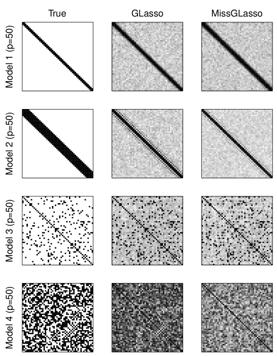
Figure 1: Heat-maps of the identified zeros in the concentration matrix $K$ among 50 simulation runs of models 1-4 with $p=50$. White color stands for zero in each of the 50 simulation runs. Black stands for non-zero in all runs. Left column: True concentration matrix. Middle column: Concentration matrix from GLasso applied on complete data. Right column: Concentration matrix from MissGLasso applied on data with $30\%$ of the values missing

Finally, we comment on initialization and computational timings of the MissGLasso. In the above simulation we used the MeanImp solution as starting values $(\mu^{(0)},K^{(0)})$ for the MissGLasso. For a typical realization of model 2 with $p=100$, $30\%$ missing data and a prediction optimal tuned parameter $\lambda$, our algorithm converges in $3.58$ seconds and $19$ EM-iterations. All computations were carried out with the statistical computing language and environment R on a AMD Phenom(tm) II X4 925 processor with 800 MHz cpu and 7.9 GB memory.

4.1.2 Simulation 2: MissGLasso under MCAR, MAR and NMAR

In the simulation of Section 4.1.1 the missing values are produced completely at random (MCAR), i.e., missingness does not depend on the values of the data. As mentioned in Section 2.2 the MissGLasso is based on a weaker assumption, namely that the data are missing at random (MAR), in the sense that the probability that a value is missing may depend on the observed values but does not depend on the missing values. A missing data mechanism where missingness depends also on the missing values is called not missing at random (NMAR), see for example Little and Rubin (1987). In this section we will show exemplarily that our method performs differently under the MCAR, MAR and NMAR assumption.

We consider a Gaussian model with $p=30$, $n=100$ and with a block-diagonal covariance matrix

$$\Sigma=\begin{bmatrix}B&0&\cdots&0\\ 0&B&&\vdots\\ \vdots&&\ddots&0\\ 0&\cdots&0&B\end{bmatrix},\qquad B=\biggl{(}\begin{smallmatrix}1&0.7&0.7^{2}\\ 0.7&1&0.7\\ 0.7^{2}&0.7&1\end{smallmatrix}\biggl{)}.$$

Note that the concentration matrix $K$ is again block-diagonal and therefore a sparse matrix.

We now delete values from the training data according to the following missing data mechanisms:

• for all $b=1,\ldots,10$ and $i=1,\ldots,n$:

  $$\mathbf{x}_{i,3\cdot b}\quad\textrm{is missing if}\quad\eta_{i,b}=1,$$

  where $\eta_{i,b}$ are i.i.d. Bernoulli random variables taking value $1$ with probability $\pi$ and 0 with probability $1-\pi$.

• for all $b=1,\ldots,10$ and $i=1,\ldots,n$:

  $$\mathbf{x}_{i,3\cdot b}\quad\textrm{is missing if}\quad\mathbf{x}_{i,3\cdot b-2}<T.$$

• for all $b=1,\ldots,10$ and $i=1,\ldots,n$:

  $$\mathbf{x}_{i,3\cdot b}\quad\textrm{is missing if}\quad\mathbf{x}_{i,3\cdot b}<T.$$

In all mechanisms the first and second variable of each block are completely observed. Only the third variable of each block has missing values. Mechanism 1 is clearly MCAR, mechanism 2 is MAR and mechanism 3 is NMAR. The probability $\pi$ and the truncation constant $T$ determine the amount of missing values. In our simulation we use three different degrees of missingness: (a) $\pi=0.25$, $T=\Phi^{-1}(0.25)$, (b) $\pi=0.5$, $T=\Phi^{-1}(0.5)=0$ and (c) $\pi=0.75$, $T=\Phi^{-1}(0.75)$. Here, $\Phi(\cdot)$ is the standard normal cumulative distribution function. Setting (a) results in about $8\frac{1}{3}\%$, (b) in $16\frac{2}{3}\%$ and (c) in $25\%$ missing data. In Figure 2, box-plots of the Kullback-Leibler loss over 50 simulation runs are shown. As expected we see that MissGLasso performs worse in the NMAR case. This observation is more pronounced for larger percentages of missing data.

Figure 2: Kullback-Leibler loss over 50 simulation runs for different missing data mechanisms (MCAR, MAR, NMAR) and different degrees of missingness: (a) $\pi=25\%$, $T=\Phi^{-1}(0.25)$, (b) $\pi=50\%$, $T=0$, (c) $\pi=75\%$, $T=\Phi^{-1}(0.75)$

4.1.3 Simulation 3: BIC and cross-validation

So far, we tuned the parameter $\lambda$ by minimizing twice the negative log-likelihood (log-loss) on validation data. However, in practice, it is more appropriate to use cross-validation or the BIC criterion presented in Section 2.3.4.

Figure 3 shows the Kullback-Leibler loss, the true positive rate and the true negative rate for the MissGLasso applied on model 1 with $p=50$. We see from the plots that cross-validation and tuning using additional validation data of size $100$ lead to very similar results. On the other hand BIC performs inferior in terms of Kullback-Leibler loss, but slightly better regarding the true negative rate.

Figure 3: KLloss, TPR, TNR of the MissGLasso estimator tuned with either additional validation data, cross-validation or BIC. Model 1 with $p=50$, $n=100$ and $10\%-30\%$ missing values, based on $50$ simulation runs

4.1.4 Scenario 4: Isoprenoid gene network in Arabidopsis thaliana

For illustration, we apply our approach for modeling the isoprenoid gene network in Arabidopsis thaliana. The number of genes in the network is $p=39$. The number of observations, corresponding to different experimental conditions, is $n=118$. More details about the data can be found in Wille et al (2004). The dataset is completely observed. Nevertheless, we produce missing values completely at random and examine the performance of MissGLasso. We consider the following experiments.

First experiment: Predictive performance in terms of log-loss.

Besides MissGLasso, MeanImp and MissRidge we consider here a fourth method based on K-nearest neighbors imputation (Troyanskaya et al, 2001). For the latter we impute the missing values by K-nearest neighbors imputation and then we estimate the inverse covariance by using GLasso on the imputed data. The number of nearest neighbors is chosen in advance in order to obtain minimal imputation error.

Based on the original data we create 50 datasets by deleting (completely at random) each time $30\%$ of the values. For each of these datasets we compute a 10-fold cross-validation error as follows: We split the dataset into 10 equal-sized parts. We fit for various $\lambda$-values the different estimators on every nine tenth of the (incomplete) dataset and evaluate the prediction error (based on out-sample negative log-likelihood) on the left-out part of the original (complete) data. The cross-validation error (cv error) is then the average over the 10 different prediction errors for an optimal $\lambda$-value. The box-plots in the left panel of Figure 4 show the cv errors over the 50 datasets. MissGLasso, MissRidge and KnnImp lead to a significant gain in prediction accuracy over MeanImp. In this example MissRidge performs best.

Second experiment: Edge selection.

First, we select using the GLasso on the original (complete) data (prediction optimal tuned) the twenty most important edges according to the estimated partial correlations given by

$$\hat{\rho}_{jj^{\prime}|\mathrm{rest}}=\frac{|\hat{K}_{jj^{\prime}}|}{\sqrt{\hat{K}_{jj}\hat{K}_{j^{\prime}\!j^{\prime}}}},\quad j,j^{\prime}=1,\ldots,p.$$

Then, we create 50 datasets by producing completely at random $m\%$ missing values and select using the MissGLasso for each of the 50 datasets the twenty most important edges according to the partial correlations $\hat{\rho}_{jj^{\prime}|\mathrm{rest}}$. We do this for $m=5,10,15,20,25,30$. Finally, we identify the overlap of the selected edges without missing values and of the selected edges with $m\%$ missing data. The box-plots in the right panel of Figure 4 visualize the size of this overlap. Even with $30\%$ missing data, the MissGLasso detects about 13 of the twenty most important edges of the complete data.

Figure 4: Arabidopsis thaliana data ($n=118,p=39$). Left panel: Cross-validation error of MeanImp, KnnImp(=K-nearest neighbors imputation followed by the GLasso), MissRidge and MissGLasso over $50$ datasets. For each dataset, $30\%$ of the original data are deleted. Right panel: Box-plots of the overlap of the twenty most important edges from GLasso and MissGLasso with and without missing values over 50 datasets

4.2 Simulations for sparse regression

4.2.1 Simulation 1

In this section we will explore the performance of the two-stage likelihood method developed in Section 3.2. In particular, we compare our new method with alternative ways of treating high-dimensional regression with missing values.

Consider the Gaussian linear model

$$Y_{i}=\beta^{T}X_{i}+\epsilon_{i},\quad i=1,\ldots,n,$$

$$\epsilon_{1},\ldots,\epsilon_{n}\quad\textrm{i.i.d.}\sim\mathcal{N}(0,\sigma^{2}),$$

where the covariates $X_{i}\in\mathbb{R}^{p},i=1,\ldots,n$, are either fixed or i.i.d. $\sim\mathcal{N}(0,\Sigma)$. In all simulations training- and validation data are generated from this model. Assuming that there are missing values only in the $\mathbf{x}$ matrix of the training data we apply one of the following methods:

• MeanImp: Impute the missing values by their corresponding column means. Then apply the Lasso-estimator (3.22) on the imputed data.

• KnnImp: Impute the missing values by the K-nearest neighbors imputation method (Troyanskaya et al, 2001). Then apply the Lasso on the imputed data.

• MissGLImp: Compute $(\hat{\mu},\hat{K})$ with the MissGLasso estimator. Then, use this estimate to impute the missing values by conditional mean imputation, i.e., replace the missing values in observation $i$ by

  $$\hat{x}_{\mathrm{mis},i}:=\mathbb{E}[x_{\mathrm{mis},i}|x_{\mathrm{obs},i},\hat{\mu},\hat{K}].$$

  Finally, apply the Lasso on the imputed data.

• Miss2stg: This is the method introduced in Section 3.2. (1st stage: solve the MissGLasso problem; 2nd stage: estimate $\beta$ and $\sigma$ by minimizing a penalized negative log-likelihood, see Equation (3.33), where we fixed $\mu$ and $K$ in the likelihood at the values from the 1st stage; initialization of EM with $\beta\equiv 0$ and $\sigma^{2}=\textrm{empirical variance of $\mathbf{y}$}$)

All methods, except for MeanImp, involve two tuning parameters. Regarding the first parameter, the number of nearest neighbors in KnnImp or the regularization parameter for the MissGLasso are chosen by cross-validation on the training data. The second tuning parameter in the Lasso or in the 2nd stage of the Miss2stg approach, respectively, are chosen to minimize the prediction error on the validation data.

To assess the performances of all methods we use the L2-distance between the estimate $\hat{\beta}$ and the true parameter $\beta$, $\|\hat{\beta}-\beta\|^{2}_{2}$.

First experiment:

Model 5:

$p=8$, $\Sigma_{jj^{\prime}}=\tau^{|j-j^{\prime}|}$ and $\beta$=(3,1.5,0,0,2,0,0,0).

We focus on four different versions of this model with different combinations of $n/\tau/\sigma$, namely $20/0.5/3$; $40/0.5/1$; $40/0.95/1$; $100/0.5/0.5$. The values $n/\tau/\sigma=20/0.5/3$ correspond to the model which was considered in the original Lasso paper (Tibshirani, 1996).

The box-plots in Figure 5 of the L2-distances, summarize the performance of the different methods for different combinations $n/\tau/\sigma$. In this experiment, 20% of the training data were deleted completely at random. For reference, we added a box-plot for the L2-distances for the Lasso carried out on complete data, i.e., before deleting 20% in the training data.

For the model from the original Lasso paper, namely the combination $n/\tau/\sigma=20/0.5/3$, we see that the Lasso on complete data does not perform substantially better than simple mean imputation on data with 20% of the values removed. This is due to the high noise level in this model. By increasing $n$ and/or scaling down $\sigma$, we reduce the noise level and increase the signal in the data. Indeed, in the setup $n/\tau/\sigma=40/0.5/1$, the analysis with complete data performs now much better than all analyses carried out on data with missing values. We also see that the Miss2stg method is slightly better than the other methods. In the setup $n/\tau/\sigma=40/0.95/1$ we increase the correlation between the covariates by setting $\tau$ from 0.5 to 0.95 and we notice that now KnnImp, MissGLImp and Miss2stg outperform the “naive” MeanImp which ignores the correlation among the different variables in the imputation step. Finally in the last setup, $n/\tau/\sigma=100/0.5/0.5$, where $n$ is increased and $\sigma$ is reduced again, the Miss2stg method is much better than the other methods. Thus, for the cases considered where missing data imply a clear information loss (e.g., when the difference between complete and mean imputed data is large), the new two-stage procedure is best.

Figure 5: Model 5. Box-plots of the L2-distances for different values for $n,\tau$ and $\sigma$ over 50 simulation runs with 20% of the training data deleted completely at random. Compl: Lasso on complete data (before deleting 20% of the data). Mean(=MeanImp): Mean imputation followed by the Lasso. Knn(=KnnImp): Knn imputation followed by the Lasso. MissGL(=MissGLImp): MissGLasso and conditional mean imputation followed by the Lasso. 2stg(=Miss2stg): Two-stage likelihood approach introduced in Section 3.2

Second experiment:

Consider the following models:

Model 6:

$n=100$; $p=50$ and $p=200$; $\Sigma_{jj^{\prime}}=0.8\times\mathrm{I}_{(j,j^{\prime}\leq 9)}$ for $j\neq j^{\prime}$, and $\Sigma_{jj}=1$; $\beta_{j}=2$ for $j=1,\ldots,8$ and zero elsewhere; $\sigma=0.5$.

Model 7:

$n=100$; $p=50$ and $p=200$; $\Sigma_{jj^{\prime}}=\mathrm{I}_{(j=j^{\prime})}$; $\beta=(3,1.5,0,0,2,0,0,0,\ldots)$; $\sigma=0.5$.

Model 8:

$n=118$; $p=39$; x: data from isoprenoid gene network in Arabidopsis thaliana (see Section 4.1.4); $\beta_{j}=2$ for $j=1,2,3$ and zero elsewhere; $\sigma=0.5$.

We delete 10%, 20% and 30% of the training data completely at random. The results (L2-distances) are reported in Table 5. We read off from this table, that the Miss2stg method performs best in all three models. We further notice that in model 7, KnnImp and MissGLImp do not perform better than simple MeanImp whereas Miss2stg works much better than all other methods. The explanation is that KnnImp and MissGLImp use the information present in the covariance matrix of $X$, which is the identity matrix for model 7, for imputation. On the other hand, our two-stage likelihood approach involves the joint distribution of $(Y,X)$ which seems to be the main reason for its better performance.

Model 6		MeanImp	KnnImp	MissGLImp	Miss2stg
$p=50$	$10\%$	2.59(0.18)	1.22(0.12)	0.42(0.04)	0.32(0.02)
	$20\%$	5.87(0.56)	2.88(0.23)	1.16(0.11)	0.96(0.08)
	$30\%$	7.05(0.47)	5.61(0.45)	2.03(0.18)	1.46(0.10)
$p=200$	$10\%$	2.55(0.23)	2.22(0.20)	0.49(0.04)	0.48(0.04)
	$20\%$	5.44(0.44)	5.16(0.42)	1.20(0.10)	1.23(0.08)
	$30\%$	8.10(0.65)	7.63(0.59)	2.00(0.18)	1.67(0.11)
Model 7		MeanImp	KnnImp	MissGLImp	Miss2stg
$p=50$	$10\%$	0.22(0.02)	0.25(0.02)	0.22(0.02)	0.05(0.00)
	$20\%$	0.56(0.05)	0.63(0.06)	0.56(0.05)	0.09(0.01)
	$30\%$	0.77(0.05)	0.92(0.06)	0.80(0.05)	0.13(0.01)
$p=200$	$10\%$	0.41(0.04)	0.41(0.03)	0.43(0.04)	0.09(0.01)
	$20\%$	0.80(0.06)	0.81(0.06)	0.86(0.07)	0.15(0.02)
	$30\%$	1.38(0.10)	1.42(0.10)	1.44(0.11)	0.57(0.08)
Model 8		MeanImp	KnnImp	MissGLImp	Miss2stg
$10\%$		1.59(0.15)	0.49(0.06)	0.29(0.04)	0.13(0.02)
$20\%$		3.04(0.17)	1.37(0.13)	0.66(0.06)	0.25(0.03)
$30\%$		4.29(0.22)	2.38(0.15)	1.30(0.12)	0.62(0.06)

Table 5: Models 6-8: Average (SE) L2-distance of MeanImp, KnnImp, MissGLImp and Miss2stg with different degrees of missingness

4.2.2 Scenario 2: Riboflavin production in Bacillus Subtilis

We finally illustrate the proposed two-stage likelihood approach on a real dataset of riboflavin (vitamin B₂) production by Bacillus Subtilis. The data has been provided by DSM (Switzerland). The real-valued response variable is the logarithm of the riboflavin production rate. There are $p=4088$ covariates (genes) measuring the logarithm of the expression level of $4088$ genes and measurements of $n=146$ genetically engineered mutants of Bacillus Subtilis. We compare the estimators MeanImp, KnnImp, MissGLImp and Miss2stg by carrying out a cross-validation analysis as in the first experiment of Section 4.1.4. Here, we use the squared error loss $(y-\beta^{T}x)^{2}$ to evaluate the prediction errors. To keep the computational effort reasonable, we use only the $100$ covariates (genes) exhibiting the highest empirical variances. The cv errors over $50$ datasets (for each dataset, $30\%$ of the complete gene expression matrix are deleted completely at random) are shown in Figure 6. MeanImp is worst. Our Miss2stg performs slightly better than KnnImp and MissGLImp.

Figure 6: Cross-validated prediction error $(y-\beta^{T}x)^{2}$ of MeanImp, KnnImp, MissGLImp and Miss2stg over 50 datasets, where for each dataset 30% of the riboflavin data are deleted

5 Discussion

We presented an $\ell_{1}$-penalized (negative) log-likelihood method for estimating the inverse covariance matrix in the multivariate normal model in presence of missing data. Our method is based on the observed likelihood and therefore works in the missing at random (MAR) setup which is more general than the missing completely at random (MCAR) framework. As argued in Section 4.1.2, the method cannot handle missingness pattern which are not at random (NMAR), i.e., ”systematic” missingness. For optimization, we use a simple and efficient EM algorithm which works in a high-dimensional setup and which can cope with high degrees of missing values. In sparse settings, the method works substantially better than $\ell_{2}$-regularization. In Section 3, the methodology was extended for high-dimensional regression with missing values in the covariates. We developed a two-stage likelihood approach which was found to be never worse but sometimes much better than K-nearest neighbors or using the straightforward imputation with a penalized covariance (and mean) estimate from incomplete data.

Appendix A Proofs

Proposition 2.1.

Denote by $f_{c}(\mathbf{x}|\mu,K)$ the multivariate Gaussian density of the complete data. $f_{\mathrm{obs}}(\mathbf{x}_{\mathrm{obs}}|\mu,K)$ the density of the observed data. Furthermore, the conditional density of the complete data given the observed data is

$$k(\mathbf{x}|\mathbf{x}_{\mathrm{obs}},\mu,K)=f_{c}(\mathbf{x}|\mu,K)/f_{\mathrm{obs}}(\mathbf{x}_{\mathrm{obs}}|\mu,K).$$

The penalized observed log-likelihood (2.10) fulfills the equation

$$-\ell_{\mathrm{pen}}(\mu,K) = -\log f_{\mathrm{obs}}(\mathbf{x}_{\mathrm{obs}}|\mu,K)+\lambda\|K\|_{1}$$ (A.36)

$$= \mathop{Q}(\mu,K|\mu^{\prime},K^{\prime})-\mathop{H}(\mu,K|\mu^{\prime},K^{\prime}),$$

where

$$\mathop{Q}(\mu,K|\mu^{\prime},K^{\prime}) = -\mathbb{E}[\ell(\mu,K;\mathbf{x})|\mathbf{x}_{\mathrm{obs}},\mu^{\prime},K^{\prime}]+\lambda\|K\|_{1}$$

$$\mathop{H}(\mu,K|\mu^{\prime},K^{\prime}) = -\mathbb{E}[\log k(\mathbf{x}|\mathbf{x}_{\mathrm{obs}},\mu,K)|\mathbf{x}_{\mathrm{obs}},\mu^{\prime},K^{\prime}].$$

By Jensen’s inequality we get the following important relationship:

$$\mathop{H}(\mu,K|\mu^{\prime},K^{\prime})\geq\mathop{H}(\mu^{\prime},K^{\prime}|\mu^{\prime},K^{\prime}),$$ (A.37)

see also Wu (1983). $\ell_{\mathrm{pen}}(\mu,K)$, $\mathop{Q}(\mu,K|\mu^{\prime},K^{\prime})$ and $\mathop{H}(\mu,K|\mu^{\prime},K^{\prime})$ are all continuous functions in all arguments. Further, $\mathop{H}(\mu,K|\mu^{\prime},K^{\prime})$ is differentiable as a function of $(\mu,K)$. If we think of $\mathop{Q}(\mu,K|\mu^{\prime},K^{\prime})$ and $\mathop{H}(\mu,K|\mu^{\prime},K^{\prime})$ as functions of $(\mu,K)$ we write also $\mathop{Q}_{(\mu^{\prime},K^{\prime})}(\mu,K)$ and $\mathop{H}_{(\mu^{\prime},K^{\prime})}(\mu,K)$.

Let $\theta^{m}=(\mu^{(m)},K^{(m)})$ be the sequence generated by the EM algorithm. We need to prove that for a converging subsequence $\theta^{m_{j}}\rightarrow\bar{\theta}$ ($j\to\infty$) the directional derivative $-\ell^{\prime}_{\mathrm{pen}}(\bar{\theta};d)$ is bigger or equal to zero for all directions $d$ (Tseng (2001)). Taking directional derivatives of Equation (A.36) yields

$$-\ell^{\prime}_{\mathrm{pen}}(\bar{\theta};d)=\mathop{Q^{\prime}_{\bar{\theta}}}(\bar{\theta};d)-\langle\nabla\mathop{H_{\bar{\theta}}}(\bar{\theta}),d\rangle.$$

Note that $\nabla\mathop{H_{\bar{\theta}}}(\bar{\theta})=0$ as $\mathop{H}_{\bar{\theta}}(x)$ is minimized for $x=\bar{\theta}$ (Equation (A.37)). Therefore, it remains to show that $\mathop{Q^{\prime}_{\bar{\theta}}}(\bar{\theta};d)\geq 0$. From the descent property of the algorithm (Equation (A.36) and (A.37)) we have:

$$-\ell_{\mathrm{pen}}(\theta^{0})\!\geq-\ell_{\mathrm{pen}}(\theta^{1})\!\geq\cdots\geq\!-\ell_{\mathrm{pen}}(\theta^{m})\geq-\ell_{\mathrm{pen}}(\theta^{m+1}).$$ (A.38)

Equation (A.38) and the converging subsequence imply that $\{\ell_{\mathrm{pen}}(\theta^{m});m=0,1,2,\ldots\}$ converges to $\ell_{\mathrm{pen}}(\bar{\theta})$. Further we have :

$$0\leq\mathop{Q_{\theta^{m}}}(\theta^{m})-\mathop{Q_{\theta^{m}}}(\theta^{m+1}) = -\ell_{\mathrm{pen}}(\theta^{m})+\ell_{\mathrm{pen}}(\theta^{m+1})+\underbrace{\mathop{H_{\theta^{m}}}(\theta^{m})-\mathop{H_{\theta^{m}}}(\theta^{m+1})}_{\leq 0}$$

$$\leq \underbrace{-\ell_{\mathrm{pen}}(\theta^{m})+\ell_{\mathrm{pen}}(\theta^{m+1})}_{\xrightarrow{m\to\infty}-\ell_{\mathrm{pen}}(\bar{\theta})+\ell_{\mathrm{pen}}(\bar{\theta})=0}.$$

The first inequality follows from the definition of the M-Step. We conclude

$$\mathop{Q_{\theta^{m}}}(\theta^{m})-\mathop{Q_{\theta^{m}}}(\theta^{m+1})\xrightarrow{m\to\infty}0.$$ (A.39)

In each M-Step we minimize the function $\mathop{Q_{\theta^{m}}}(x)$ with respect to $x$. Therefore we have:

$$\underbrace{\mathop{Q_{\theta^{m_{j}}}}(\theta^{m_{j}+1})-\mathop{Q_{\theta^{m_{j}}}}(\theta^{m_{j}})}_{\xrightarrow{j\to\infty}0\quad(\ref{eq:eq4})}+\underbrace{\mathop{Q_{\theta^{m_{j}}}}(\theta^{m_{j}})}_{\xrightarrow{j\to\infty}\mathop{Q_{\bar{\theta}}}(\bar{\theta})}\leq\underbrace{\mathop{Q_{\theta^{m_{j}}}}(x)}_{\xrightarrow{j\to\infty}\mathop{Q_{\bar{\theta}}}(x)}.$$ (A.40)

Using continuity, Equation (A.39) and Equation (A.40) we get

$$\mathop{Q_{\bar{\theta}}}(\bar{\theta})\leq\mathop{Q_{\bar{\theta}}}(x)\qquad\forall x$$

and therefore, we have proven that $\mathop{Q^{\prime}_{\bar{\theta}}}(\bar{\theta};d)\geq 0$ for all directions $d$. ∎

Proposition 3.1.

The result follows from Proposition 5.1 and Lemma 3.1 in Tseng (2001). ∎

Lemma 3.1.

We have

$$(\epsilon_{i},X_{i})\!\sim\!\mathcal{N}\left(\!(0,\mu),\left(\!\begin{array}[]{cc}\sigma^{2}&0\\ 0&\Sigma\end{array}\!\right)\!\right)\,\textrm{and}\,\left(\!\begin{array}[]{c}Y_{i}\\ X_{i}\end{array}\!\right)\!=\!\left(\begin{array}[]{cc}1&\beta^{T}\\ 0&1\end{array}\right)\!\left(\!\begin{array}[]{c}\epsilon_{i}\\ X_{i}\end{array}\!\right).$$ (A.49)

From (A.49) we see that the joint distribution of $(Y_{i},X_{i})$ follows a (p+1)-variate normal distribution with mean and covariance given by

$$\tilde{\mu}=(\beta^{T}\mu,\mu),\qquad\widetilde{\Sigma}=\left(\begin{array}[]{cc}\sigma^{2}\!+\!\beta^{T}\!\Sigma\beta&\beta^{T}\!\Sigma\\ \Sigma\beta&\Sigma\end{array}\right).$$

The expression for the concentration matrix $\widetilde{K}=\widetilde{\Sigma}^{-1}$ can be derived by using the identity $\widetilde{\Sigma}\widetilde{K}=I$. ∎

Acknowledgements N.S. acknowledges financial support from Novartis International AG, Basel, Switzerland.

References

- Banerjee et al (2008) Banerjee O, El Ghaoui L, d’Aspremont A (2008) Model selection through sparse maximum likelihood estimation for multivariate Gaussian or Binary data. Journal of Machine Learning Research 9:485–516
- Buck (1960) Buck S (1960) A method of estimation of missing values in multivariate data suitable for use with an electronic computer. Journal of the Royal Statistical Society B 22:302–306
- Dempster et al (1977) Dempster A, Laird N, Rubin D (1977) Maximum likelihood from incomplete data via the EM algorithm. Journal of the Royal Statistical Society, Series B 39:1–38
- Friedman et al (2007a) Friedman J, Hastie T, Hoefling H, Tibshirani R (2007a) Pathwise coordinate optimization. Annals of Applied Statistics 1:302–332
- Friedman et al (2007b) Friedman J, Hastie T, Tibshirani R (2007b) Sparse inverse covariance estimation with the graphical Lasso. Biostatistics 9:432–441
- Friedman et al (2010) Friedman J, Hastie T, Tibshirani R (2010) Regularized paths for generalized linear models via coordinate descent. Journal of Statistical Software 33(1):1–22
- Ibrahim et al (2008) Ibrahim JG, Zhu H, Tang N (2008) Model selection criteria for missing-data problems using the EM algorithm. Journal of the American Statistical Association 103(484):1648–1658
- Lauritzen (1996) Lauritzen S (1996) Graphical Models. Oxford University Press
- Little and Rubin (1987) Little RJA, Rubin D (1987) Statistical Analysis with Missing Data. Series in Probability and Mathematical Statistics, Wiley
- Meinshausen (2008) Meinshausen N (2008) A note on the Lasso for Gaussian graphical model selection. Statistics & Probability Letters 78(7):880–884
- Meinshausen and Bühlmann (2006) Meinshausen N, Bühlmann P (2006) High dimensional graphs and variable selection with the Lasso. Annals of Statistics 34:1436–1462
- Murray (1977) Murray GD (1977) Comments on “Maximum likelihood from incomplete data via the EM algorithm” by Dempster, Laird, and Rubin. Journal of the Royal Statistical Society, Series B 39:27–28
- Ravikumar et al (2008) Ravikumar P, Wainwright M, Raskutti G, Yu B (2008) High-dimensional covariance estimation by minimizing -penalized log-determinant divergence. Arxiv preprint arXiv:0811.3628v1 [statML]
- Rothman et al (2008) Rothman A, Bickel P, Levina E, Zhu J (2008) Sparse permutation invariant covariance estimation. Electronic Journal of Statistics 2:494–515
- Schafer (1997) Schafer JL (1997) Analysis of Incomplete Multivariate Data. Monographs on Statistics and Applied Probability 72, Chapman and Hall
- Städler et al (2010) Städler N, Bühlmann P, van de Geer S (2010) -penalization for mixture regression models (with discussion). Test 19(2):209–285
- Tibshirani (1996) Tibshirani R (1996) Regression shrinkage and selection via the Lasso. Journal of the Royal Statistical Society, Series B 58:267–288
- Troyanskaya et al (2001) Troyanskaya O, Cantor M, Sherlock G, Brown P, Hastie T, Tibshirani R, Botstein D, Altman RB (2001) Missing value estimation methods for DNA microarrays. Bioinformatics 17(6):520–525
- Tseng (2001) Tseng P (2001) Convergence of a block coordinate descent method for nondifferentiable minimization. Journal of Optimization Theory and Applications 109:475–494
- Wille et al (2004) Wille A, Zimmermann P, Vranova E, Fürholz A, Laule O, Bleuler S, Hennig L, Prelic A, von Rohr P, Thiele L, Zitzler E, Gruissem W, Bühlmann P (2004) Sparse graphical Gaussian modeling of the isoprenoid gene network in arabidopsis thaliana. Genome Biology 5(11):R92
- Witten and Tibshirani (2009) Witten DM, Tibshirani R (2009) Covariance-regularized regression and classification for high-dimensional problems. Journal of the Royal Statistical Society, Series B 71(3):615–636
- Wu (1983) Wu C (1983) On the convergence properties of the EM algorithm. Annals of Statistics 11:95–103
- Yuan and Lin (2007) Yuan M, Lin Y (2007) Model selection and estimation in the Gaussian graphical model. Biometrika 94:19–35