The triple Pomeron vertex in large-$\bm{N}_{c}$ QCD
and the pair-of-pants topology

Abstract

We investigate the high energy behavior of QCD for different surface topologies of color graphs. After a brief review of the planar limit (bootstrap and gluon reggeization) and of the cylinder topology (BFKL) we investigate the $3\to 3$ scattering in the triple Regge limit which belongs to the pair-of-pants topology. We re-derive the triple Pomeron vertex function and show that it belongs to a specific set of graphs in color space which we identify as the analogue of the Mandelstam diagram.

1 Introduction

Starting from the classical paper by ’t Hooft [1] the large $N_{c}$ limit of gauge theories has remained in the center of attention for more than 25 years. In high energy QCD-phenomenology for instance, the large-$N_{c}$ expansion proves its usefulness as a simplifying tool, if one attempts to resum higher order contributions, enhanced by large logarithms. With the general structure of the color factors being often too complex, the large $N_{c}$ limit allows for resummation with an acceptable reduction of accuracy.

A new attraction of the large $N_{c}$ expansion results nowadays from the fact that it organizes the color structure of Feynman diagrams in terms of topologies of two-dimensional surfaces which resemble the loop expansion of a closed string theory. With the advance of the AdS/CFT correspondence [2] which, in the limit of large $N_{c}$, connects $N=4$ Super-Yang-Mills theory with a closed string theory in Anti-de-Sitter space and with string coupling proportional to $N_{c}^{-1}$ this idea is more prevailing than ever.

The leading term of the large $N_{c}$ expansion is given by color factors that have the topology of the sphere or equivalently the plane, and one usually refers to these leading contributions as ’planar’ diagrams. Planar diagrams contribute, for example, to gluon-gluon scattering amplitudes or to multi-gluon production amplitudes. On the other hand, there exist also processes where the $N_{c}$ leading color factor has not the topology of the plane. This is, for instance, the case for the scattering of two electromagnetic currents or virtual photons at high energies where the center of mass energy squared $s$ is far bigger than the momentum transfer squared and the virtualities of the photons. In this case, the interaction between the scattering currents is mediated by the exchange of gluons between two quark loops, and, with quarks in QCD in the fundamental representation of the gauge group $SU(N_{c})$, the leading color factor has the topology of a sphere with two boundaries, a cylinder. Within perturbative QCD such processes, at leading [3] and next-to-leading order accuracy [4], are described by the BFKL-Pomeron, which is a bound state of two reggeized gluons. Higher order unitarity corrections are expected to involve bound states of more than 2 reggeized gluons, so called BKP-states [5], which for the cylinder topology have been found to be integrable [6].

In the present study we go one step further and consider the class of process whose leading color factor has the topology of a sphere with three boundaries.

 

Figure 1: The ’pair of pants’ topology

 

Figure 2: Typical contributions to the triple energy discontinuity for scattering of three virtual photons

Such a surface is depicted in Fig.2 and it is usually referred to as the topology of a ’pair of pants’. As a suitable example we consider the three-to-three process which describes the scattering of a highly virtual photon on two virtual photons in the triple Regge limit. Similar to the BFKL-Pomeron on the cylinder, we resum all contributions which are maximally enhanced by logarithms of energies. The class of diagrams selected in this way is illustrated in Fig.2: the three photon impact factors introduce three boundaries, and thus belong to the topology depicted in Fig.2. Compared to the simple BFKL cylinder, the new feature is the splitting of one cylinder into two cylinders which is related to the ’triple Pomeron vertex’ [7]. Within the AdS/CFT correspondence, the electromagnetic current corresponds to the R-current, and the high energy behavior of the 6-point amplitude, on the string side, is expected to exhibit the triple graviton vertex.

In QCD this $3\to 3$ process has been investigated before for $N_{c}=3$ in [7], the triple Pomeron vertex has been derived, and it has been shown to be invariant under two-dimensional Möbius transformations [8]. It is straightforward to repeat the analysis for arbitrary $N_{c}$ and to take the large-$N_{c}$ limit of these calculations. The system of four reggeized gluons and the triple Pomeron vertex have been further investigated particularly for the limit $N_{c}\to\infty$ in [9, 10]. However the connection of these results with the expansion in terms of topologies of two-dimensional surfaces is not apparent. Instead of the pair-of-pants, the color factor rather seems to correspond to three disconnected cylinders. In the present paper, we therefore demonstrate that by summing only diagrams with the topology of the pair-of-pants, Fig.2, one obtains the result of the large-$N_{c}$ limit of [7]. In particular we find that the ’reggeizing’ and ’irreducible’ terms of [7] can be attributed to distinct classes of diagrams on the surface of the pair-of-pants.

Our paper is organized as follows. In section 2 we briefly review the planar and cylinder topologies. In the high energy limit, the planar diagrams satisfy the bootstrap condition of the reggeizing gluon, whereas the cylinder diagrams lead to the famous BFKL amplitude. In section 3 we turn to the analytic form of the $3\to 3$ scattering amplitude and give a general description of the diagrams which need to be summed. In Section 4 we study the color lines on the surface of the pants, arriving at the definition of two distinct classes of diagrams in color space (named ’planar’ and ’non-planar’). We also review the different momentum space kernels which describe the interactions of reggeized gluons. In section 5 we sum the ’planar’ diagrams and arrive at the ’reggeized’ amplitudes introduced in [7], whereas in the section 6 we investigate the ’non-planar’ diagrams and re-derive the triple Pomeron vertex of [7]. In section 7 we briefly summarize our results, and the final section 8 contains a few conclusions.

2 Elastic amplitudes

In this section we begin by recalling the definition of the large $N_{c}$ expansion, following the classical paper by ’t Hooft [1]. As a preparation for the study of the pair-of-pants topology, we then reconsider the simplest examples of diagrams, whose color factor have the topology of the plane and of the cylinder. In the Regge-limit they yield the reggeized gluon and the BFKL-Pomeron, respectively.

2.1 The large $N_{c}$ expansion

To study the large $N_{c}$ limit as an expansion of topologies of the color factor, one is asked to translate the color factors of a scattering amplitude into the so-called double line notation. To this end we use the $SU(N_{c})$ generators in the fundamental representation, $(g^{a})^{i}_{j}$, in the normalization ${\rm tr}(g^{a}g^{b})=\delta^{ab}$, and we make use of the identity

$$f^{abc} =\frac{1}{i\sqrt{2}}\big{[}{\rm tr}(g^{a}g^{b}g^{c})-{\rm tr}(g^{c}g^{b}g^{a})\big{]}.$$ (1)

For all inner gluon lines in the adjoint representation, the indices can then be expressed in terms of (anti-)fundamental indices by means of the Fierz identity

$$(g^{a})^{i}_{j}(g^{a})^{k}_{l}=\delta^{i}_{l}\delta^{k}_{j}-\frac{1}{N_{c}}\delta^{i}_{j}\delta^{k}_{l}.$$ (2)

Making use of a diagrammatic notation, where a Kronecker-delta is represented by a single line with an arrow, indicating the flow from the upper to the lower index,

$$\delta^{i}_{j}=\parbox{56.9055pt}{\includegraphics[width=56.9055pt]{delta.ps}},$$ (3)

the structure constants $f^{abc}$ are expressed as

$$f^{a_{1}a_{2}a_{3}}(g^{a_{1}})^{i_{1}}_{j^{1}}(g^{a_{2}})_{j_{2}}^{i^{2}}(g^{a_{3}})_{j_{3}}^{i^{3}}=\frac{1}{i\sqrt{2}}\left(\,\,\parbox{28.45274pt}{\includegraphics[height=56.9055pt]{structure1.ps}}-\parbox{36.98866pt}{\includegraphics[height=56.9055pt]{structure2.ps}}\right).$$ (4)

In order to arrive at the large $N_{c}$ expansion, one drops, in the Fierz-identity Eq.(2), the second term. As a consequence, the gluon is represented by a double line

$$\delta^{i}_{l}\delta^{k}_{j}=\parbox{56.9055pt}{\includegraphics[width=56.9055pt]{double.ps}}.$$ (5)

The neglect of second term of the Fierz-identity Eq.(2) which serves to subtract the trace of the $SU(N_{c})$ gluon implies that we consider an $U(N_{c})$ gluon rather than an $SU(N_{c})$ gluon. While this term is suppressed for large $N_{c}$, dropping this term is only correct as long as we stay within the leading term of the expansion. Tracelessness of the $SU(N_{c})$ gluon can be taken into account by introducing an additional $U(1)$ ghost field [11, 12], which subtracts the trace of the $U(N_{c})$-gluon. Since the $U(1)$ ghost-field commutes with the $U(N_{c})$ gluon-field, it couples only to quarks, but not to gluons. Within the Leading Logarithmic Approximation, which we will use in the following, the interaction between scattering objects is mediated only by gluons, while quarks occur in the coupling of the gluons to the scattering objects. Corrections due to the $U(1)$ ghost in this approximation therefore appear only in low orders of the strong coupling and are taken into account easily.

Using the double line representation for gluons, Eq.(5), and representing quarks in the fundamental representation by single lines, the color factor of a vacuum Feynman diagram turns into a network of double and single lines, which can be drawn on a two-dimensional surface with Euler number $\chi=2-2h-b$, where $h$ is the number of handles of the surface, and $b$ the number of boundaries or holes. A closed color-loop always delivers a factor $N_{c}$. With quarks being represented by single lines, a closed quark-loop, compared to a corresponding gluon-loop, is $1/N_{c}$ suppressed and leads always to a boundary. For an arbitrary vacuum graph $T$ one arrives at the following expansion in $N_{c}$

$$T=\sum_{h,b}^{\infty}N_{c}^{2-2h-b}T_{h,b}(\lambda).$$ (6)

where

$$\lambda =g^{2}N_{c}$$ (7)

is the ’t Hooft-coupling which is held fixed, while $N_{c}$ is taken to infinity. The expansion Eq.(6) matches the loop expansion of a closed string theory with the string coupling $1/N_{c}$. For $N_{c}\to\infty$, the leading diagrams are those that have the topology of a sphere: zero handles and zero boundaries, $h=b=0$. If quarks are included, the leading diagrams have the topology of a disk, i.e. the surface with zero handle and one boundary, $h=0,b=1$. The disk fits on the plane, with the boundary as the outermost edge. Diagrams with two boundaries and zero handles can be drawn on the surface of a cylinder, those with three boundaries on the surface of a pair-of-pants. Boundaries are also be obtained by removing, from the sphere, one or more points: removing one point, one obtains the disk, which can be drawn on the plane, and by identifying the removed point with infinity, the graphs can be drawn on the (infinite) plane. Removing two points we obtain the cylinder and so on. By definition, the expansion Eq.(6) is defined for vacuum graphs. However, from the earliest days on [13], the large $N_{c}$-limit has been also applied to the scattering of colored objects. In order to consider the topological expansion of an amplitude with colored external legs, one needs to embed it into a vacuum graph which then defines the topological expansion of an amplitude with colored external legs.

In the following it will be convenient to define modified couplings

$$\bar{g}=\frac{g}{\sqrt{2}},\hskip 85.35826pt\bar{\lambda}=\bar{g}^{2}N_{c}=\frac{g^{2}N_{c}}{2},$$ (8)

which absorb the factor $1/\sqrt{2}$. Due to our normalization of $SU(N_{c})$ generators which differs from the more standard one, ${\rm tr}(t^{a}t^{b})=\delta^{ab}/2$, such a factor $1/\sqrt{2}$ arises for each quark-gluon coupling and, because of Eq.(4), also for each gluon-gluon coupling.

2.2 Planar amplitudes: Reggeization of the gluon

In the present paragraph, we shall discuss the Regge-limit of planar amplitudes (first addressed in [14]) which satisfy the bootstrap condition of the reggeized gluon, the basic ingredient for the further studies. In order to study reggeization of the gluon, one considers the scattering of colored objects. To be definite, we consider the scattering of a quark on an anti-quark. The disk-topology of the color factors becomes apparent, if we connect color lines of the incoming quark and antiquark with each other and of the outgoing quark and antiquark (note that, if instead we would connect the color lines of the ingoing and outgoing quark with each other and of the incoming and outgoing antiquark, we would discover the cylinder topology). As far as the momentum part of the diagrams is concerned, our method is the following: We consider the Regge limit $s\gg-t$ of the elastic amplitude and make use of the Leading Logarithmic Approximation (LLA), where we select all diagrams that are maximally enhanced by a logarithm in $s$, i.e. that are proportional to $\frac{\lambda}{N_{c}}(\lambda\ln s)^{n}$, and sum them up to all orders in $\lambda$. Furthermore, in this approximation, all $t$-channel particles are gluons (quark exchanges are power suppressed).

We start by considering tree- and one-loop-level diagrams within the LLA, and convince ourselves that these leading order result, for planar color graphs, satisfy the bootstrap condition and are thus in agreement with the reggeization of the gluon. At tree level, the (anti-)quarks interact by exchange of a single gluon. In the standard adjoint notation, the color factor of the diagram is given by $(g^{a})^{i}_{j}(g^{a})^{l}_{k}$, which in the double-line notation turns into $\delta^{i}_{k}\delta^{l}_{j}$, while the $U(1)$-ghost can be disregarded for the plane. We therefore have

$$=\parbox{42.67912pt}{\includegraphics[width=42.67912pt]{qqbar_tree_nc.eps}}\times T^{\text{tree}}_{q\bar{q}}(s,t), T^{\text{tree}}_{q\bar{q}}(s,t) =2\bar{g}\frac{-s}{t}\bar{g}.$$ (9)

From now on we adopt the following notation: in a Feynman diagram gluons are usually denoted by curly lines, and in this notation the diagram is understood to represent both the color factors and the momentum part. Alternatively, when drawing a diagram with the double line notation for each gluon, this diagram represents only the color part, and the momentum part has to be written separately.

Turning to higher order graphs, we have the restriction that, with every insertion of an additional internal loop coming with a factor $g^{2}$, we have to produce a closed color loop, yielding a factor $N_{c}$ which then combines to the ’t Hooft coupling $\lambda=g^{2}N_{c}$. Only such higher order term will be included into the planar approximation discussed in this section. This restriction holds also for other topologies in the expansion Eq.(6): every insertion of an additional gluon into the Born diagram provides automatically a factor $g^{2}$ and must be compensated by a closed color loop in order to stay within the considered coefficient $T_{h,b}$ of the expansion. For our planar loop, for each higher order graph the tensorial structure of the color factor will be proportional to the one of the Born term. As far as the momentum part is concerned, the 1-loop diagrams for quark-antiquark scattering that contribute within the LLA are shown in Fig.3.

:     = $N_{c}$

 

:    

Figure 3: One-loop corrections to quark-antiquark scattering. On the left hand side, the color factor of the planar Feynman diagram is $N_{c}$ times the Born color factor. On the right hand side, the non-planar diagram does not fit onto the plane and is $N_{c}$ suppressed.

For both diagrams, the momentum part is of the same order of magnitude, i.e. it is proportional to $g^{2}s\ln(-s)$ and $g^{2}u\ln(-u)$, respectively, with $u\simeq-s$ in the Regge limit. However, when counting closed color loops, one sees that only the first diagram is leading in $N_{c}$. Also, when closing the color lines of the incoming quark and antiquark and of the outgoing particles, we observe that for the first diagram the ’closed’ color factor, indeed, fits on the disk with $h=0,b=1$, while the second ’closed’ color factor has an additional handle $h=1,b=1$. We therefore find for the quark-antiquark scattering amplitude at 1-loop:

$$T_{q\bar{q}}^{\text{1-loop}}(s,t) =\ln(-s)\beta(t)T_{q\bar{q}}^{\text{tree}}(s,t) \beta(-{\bf q}^{2}) =\bar{\lambda}\int\frac{d^{2}{\bf k}}{(2\pi)^{3}}\frac{-{\bf q}^{2}}{{\bf k}^{2}({\bf q}-{\bf k})^{2}},$$ with (10)

where the color factor $N_{c}$ has already been included into the gluon trajectory function, and bold letters denote Euclidean momenta perpendicular to the light-like momenta $p_{1}$ and $p_{2}$ of the scattering quark and antiquark; in particular $t=-{\bf q}^{2}$. Eq.(10) can be understood as the order $\mathcal{O}(g^{4})$ term of the expansion of the exchange of a planar reggeized gluon:

$$T_{q\bar{q}}(s,t) =2\bar{g}(-s)^{1+\beta(t)}\frac{1}{t}\bar{g}.$$ (11)

For our further analysis we use the following analytic representation of the planar elastic amplitude in the Regge limit:

$$T_{2\to 2}(s,t)=s\int_{\sigma-i\infty}^{\sigma+i\infty}\frac{d\omega}{2\pi i}s^{\omega}\xi(\omega)\phi(\omega,t).$$ (12)

The partial wave amplitude $\phi(\omega,t)$ is a real-valued function, and phases are contained in the signature factor $\xi(\omega)$:

$$\xi(\omega)=-\pi\frac{e^{-i\pi\omega}}{\sin(\pi\omega)}.$$ (13)

Note the difference from the ’usual’ signature factor $\xi\sim{e^{-i\pi\omega}}\pm 1$ which contains both right and left hand energy cuts: at one loop we have shown that only the Feynman diagram with the $s$-channel discontinuity belongs to the planar approximation whereas the $u$ discontinuity is absent. For quark-antiquark-scattering, this also holds for higher order terms. We then take the discontinuity in $s$

$$\Im\text{m}_{s}T_{2\to 2}(s,t)=\mathrm{disc}_{s}T_{2\to 2}(s,t)=\pi s\int\frac{d\omega}{2\pi i}s^{\omega}\phi(\omega,t),$$ (14)

which, by unitarity

$$2\Im\text{m}_{s}T_{2\to 2}(s,t)=\sum\int T_{2\to n}T_{2\to n}^{*}$$ (15)

relates the Mellin transform of the partial wave amplitude $\phi(\omega,t)$ to the sum of production processes. To leading order in $g$, the partial wave has the form

$$\phi^{(0)}(\omega,t)=\frac{2}{\omega}\phi_{(2;0)}\otimes\phi_{(2;0)}=\frac{2\bar{g}^{2}}{\omega t}\beta(t)$$ (16)

where $\phi_{(2;0)}=\bar{g}^{2}N_{c}^{1/2}$ denotes the non-singlet two gluon impact factor for quark and antiquark, and the convolution symbol is defined as

$$\otimes=\int\frac{d^{2}{\bf k}}{(2\pi)^{3}{\bf k}_{1}^{2}{\bf k}_{2}^{2}}$$ (17)

with ${\bf q}={\bf k}_{1}+{\bf k}_{2}$ and $t=-{\bf q}^{2}$. Higher order corrections involve diagrams where additionally real gluons are produced. To leading logarithmic accuracy, real particle production takes place within the Multi-Regge-Kinematics (MRK), where the produced particles are widely separated in rapidity. The leading order diagram, with one additional $s$-channel gluon, is illustrated in Fig.4:

Figure 4: $s$-channel discontinuity with three real particles. To the right the corresponding planar color factor.

Here the particle production vertex (depicted by a dot) is an effective vertex for the production of one real gluon. This production vertex is build by the following Feynman diagrams:

$$=\parbox{42.67912pt}{\includegraphics[width=42.67912pt]{lipatovantiquark1.eps}} + + + +$$

$$\frac{1}{i}\bigg{(}\parbox{28.45274pt}{ \includegraphics[width=28.45274pt]{prod_gross1.eps}}-\parbox{28.45274pt}{ \includegraphics[width=36.98866pt]{prod_gross1b_bow1.eps}}\bigg{)} \frac{-1}{i}\parbox{34.14322pt}{ \includegraphics[width=28.45274pt]{prod_gross2b.eps}} \frac{1}{i}\parbox{28.45274pt}{\includegraphics[width=28.45274pt]{prod_gross2.eps}} \frac{1}{i}\parbox{28.45274pt}{\includegraphics[width=28.45274pt]{prod_gross3.eps}} \frac{-1}{i}\parbox{28.45274pt}{\includegraphics[width=28.45274pt]{prod_gross3b.eps}.}$$ (18)

In the second line we show, for each of the five different Feynman-diagrams, the corresponding color factor in the double-line notation. For the last four diagrams on the right hand side, where the real gluon is emitted from the quark and the antiquark respectively, we have shifted factors $i$ and $(-i)$ from the momentum part to the color factor. With such a shift, the (remaining) momentum parts of the second and the third diagram and the momentum parts of the fourth and the fifth diagram coincide in the considered kinematical regime with each other. Color factors and momentum parts of the production vertex can therefore be written in a factorized form, and we obtain

$$=\frac{{\bar{g}}}{i}\left(\quad\parbox{28.45274pt}{\includegraphics[height=34.14322pt]{prod_gross1.eps}}\quad-\quad\parbox{28.45274pt}{ \includegraphics[height=34.14322pt]{prod_gross1b_bow1.eps}}\quad\right)\quad\times C(l,k)\cdot\epsilon_{(\lambda)},$$ (19)

where $\lambda$ denotes the helicity of the produced gluon. With the light-like momenta of the quark and the antiquark given by $p_{1}$ and $p_{2}$ respectively we have with $s\simeq 2p_{1}\cdot p_{2}$,

$$C^{\mu}(l,k)=\left(\alpha_{l}+2\frac{{\bf l}^{2}}{\beta_{k}s}\right)p_{1}^{\mu}+\left(\beta_{k}+2\frac{{\bf k}^{2}}{\alpha_{l}s}\right)p_{2}^{\mu}-(l_{\perp}^{\mu}+k_{\perp}^{\mu}),$$ (20)

where $\alpha_{l}s=2p_{2}\cdot l$ and $\beta_{k}s=2p_{1}\cdot k$. When squaring the production amplitude, we find for the color part that only one of the four possible combinations fits on the plane, namely the one shown on the right hand side of Fig.4. From the point of view of Feynman-diagrams, the planar approximation includes only a sub-set of the diagrams in Eq.(2.2), namely those with the color structure

$$\parbox{56.9055pt}{\centering\includegraphics[width=34.14322pt]{prod_gross1.eps}\@add@centering}+\parbox{56.9055pt}{\centering\includegraphics[width=34.14322pt]{prod_gross2.eps}\@add@centering}+\parbox{56.9055pt}{\centering\includegraphics[width=34.14322pt]{prod_gross3.eps} \@add@centering}$$ (21)

However due to the factorization of momentum and color parts in the MRK, Eq.(19), we still recover the complete production vertex $C_{\mu}$ and therefore the BFKL kernel. Making use of our re-defined couplings $\bar{g}$ and $\bar{\lambda}$, and including the factors $1/i$ of Eq.(19), we find, for the plane, the $2\to 2$ Reggeon transition kernel $K_{2\to 2}$ as:

$$\parbox{56.9055pt}{\includegraphics[width=51.21504pt]{k22_cut_label_gluon.eps}}=\bar{\lambda}K_{2\to 2}({\bf l}_{1},{\bf l}_{2};{\bf k}_{1},{\bf k}_{2})=-\bar{\lambda}\big{[}({\bf k}_{1}+{\bf k}_{2})^{2}-\frac{{\bf l}_{1}^{2}{\bf k}_{2}^{2}}{({\bf k}_{1}-{\bf l}_{1})^{2}}-\frac{{\bf l}_{2}^{2}{\bf k}_{1}^{2}}{({\bf k}_{1}-{\bf l}_{1})^{2}}\big{]}$$ (22)

with the constraint ${\bf l}_{1}+{\bf l}_{2}={\bf k}_{1}+{\bf k}_{2}={\bf q}$.

Higher order terms with the production of $n$-gluons within the MRK are taken into account in a similar way. Making use of Regge-factorization of the production amplitudes, it can be shown that each emission of an additional real gluon is taken into account by insertion of the effective production vertex Eq.(19), as illustrated in Fig.5 for the squared production amplitude. Similar to the production of one-gluon, for each of the inserted production vertices only one of the four possible combinations of color factors fits onto the plane, and the resulting color factor can be found on the right-hand-side of Fig.5.

Figure 5: The s-channel discontinuity of the elastic quark-antiquark scattering amplitude for three gluon production. On the right, the color structure of the planar diagrams.

In order to obtain the complete expression of order $\lambda^{n}$ of the partial wave $\phi$, we need to include the reggeization of the gluon. This is done in the same way as in the finite-$N_{c}$ case, except that at each step we have to restrict ourselves to the planar approximation. In lowest order we return, on the rhs of the unitarity equation (15), to the elastic intermediate state and include, in one of the two factors $T_{2\to 2}$, the one loop result (10). Together with the real one-gluon production discussed above, this provides, in (11), the complete imaginary part to order $g^{6}$ (or $\lambda^{3}$). Compared to the tree diagram expression (9), (11) replaces the exchange of an elementary $t$-channel gluon by a reggeized gluon. In higher order $g$, the analogous replacement has to be done, on the rhs of (15), for all $t$-channel exchanges in the production amplitudes $T_{2\to n}$.

In order to prove the self-consistency of this procedure , one has to show that the BFKL bootstrap condition is satisfied in the planar approximation. For the partial wave in Mellin-space, reggeization of the $t$-channel gluons within the LLA requires to introduce, for every $t$-channel state of two gluons, a Reggeon-propagator $1/(\omega-\beta({\bf k})-\beta({\bf q}-{\bf k}))$. In order to perform the resummation of all production processes in Fig.5, it is most convenient to formulate the BFKL integral-equation in the planar approximation. To this end we first factorize off, at the lower end of the ladder, the antiquark-impact factor $\phi_{(2;0)}$. We then define, for the scattering of a quark on a reggeized gluon, the amplitude $\phi_{2}(\omega|{\bf k}_{1},{\bf k}_{2})$, which contains the Reggeon propagator $1/(\omega-\beta({\bf{k}}_{1})-\beta({\bf{k}}_{2}))$ of the two reggeized gluons at the lower end. The BFKL-equation for this amplitude reads:

$$\big{(}\omega-\sum_{i}^{2}\beta({\bf{k}}_{i})\big{)}\phi_{2}(\omega|{\bf k}_{1},{\bf k}_{2}) =\phi_{(2;0)}({\bf k}_{1}+{\bf k}_{2})+\bar{\lambda}K_{2\to 2}\otimes\phi_{2}(\omega|{\bf k}_{1},{\bf k}_{2}),$$ (23)

where the kernel coincides with the finite $N_{c}$ case. With our impact factor $\phi_{(2;0)}$ which depends only on the sum of the transverse momenta of the $t$-channel gluons we find for Eq. (23) the familiar pole solution

$$\phi_{2}(\omega|{\bf k}_{1}+{\bf k}_{2})= \frac{\phi_{(2;0)}}{\omega-\beta(-({\bf k}_{1}+{\bf k}_{2})^{2})}.$$ (24)

The partial wave for quark-antiquark scattering becomes

$$\phi(\omega,t)=2\int\frac{d^{2}{\bf l}}{(2\pi)^{3}}\frac{1}{{\bf l}_{1}^{2}{\bf l}_{2}^{2}}\frac{\phi_{(2;0)}\phi_{(2;0)}}{\omega-\beta(t)}=\frac{1}{t}\frac{2\bar{g}^{2}\beta(t)}{\omega-\beta(t)}.$$ (25)

Inserting this into Eq.(12) and using that in LLA $\sin\pi\omega\simeq\pi\omega$, we find the reggeized gluon, as proposed in Eq.(11). This proves that, in the planar approximation, the bootstrap property is satisfied.

2.3 Cylinder topology: The BFKL-Pomeron

Next we turn to the cylinder topology which, in the Regge-limit, leads to the BFKL-Pomeron. In the expansion Eq.(6), this corresponds to the term with two boundaries and zero handles, $b=2,h=0$. Even though it would be possible to carry out this analysis for quark-antiquark scattering, it is more natural to do so for scattering of two highly virtual photons, which provides an IR-finite and gauge-invariant amplitude. Reggeization of the gluon will be an important ingredient in this analysis, as we will see in short.

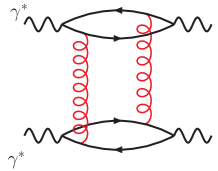
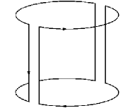
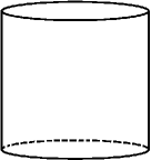
Figure 6: To the left, a typical leading order diagram with its double-line color line factor in the middle. The color factor fits on the cylinder surface, depicted to the right.

As a physical process with such a topology we consider the scattering of two highly virtual photons in the Regge limit $s\gg|t|$, and again we use the LLA to sum to all orders those diagrams which have one power of $\ln s$ for each loop. In particular, the interaction between the two photons is mediated by gluons in the $t$-channel, and to lowest order in the electromagnetic coupling, each photon couples to a quark-loop. The quark-loops provide the two boundaries of the cylinder. To leading order, the two photons interact by the exchange of two $t$-channel gluons. A typical leading order diagram is shown in Fig.6, together with its color factor. Unlike the planar case, color factors of diagrams with both discontinuities in the $s$- and in the $u$-channel fit on the cylinder. The $t$-channel-interaction has therefore positive signature, similar to the $N_{c}$ finite case,

To resum higher order terms we use again the analytic representation Eq.(12) of the elastic amplitude in the Regge limit. Now the signature factor includes both right and left hand cuts:

$$\xi(\omega)=-\pi\frac{e^{-i\pi\omega}-1}{\sin(\pi\omega)}$$ (26)

and belongs to positive signature in the $t$-channel. As in the previous paragraph, we take the discontinuity in $s$ which allows to determine the partial wave amplitude by considering real particle production processes. Coupling of the two gluon state to the virtual photon is described by the two gluon impact factor of the virtual photon which is given by the sum of the following four Feynman diagrams:

$${D}_{(2;0)}({\bf k}_{1},{\bf k}_{2})=\parbox{71.13188pt}{\includegraphics[width=71.13188pt]{gamma_impact1.eps}}+\parbox{71.13188pt}{\includegraphics[width=71.13188pt]{gamma_impact2.eps}}+\parbox{71.13188pt}{\includegraphics[width=71.13188pt]{gamma_impact3.eps}}+\parbox{71.13188pt}{\includegraphics[width=71.13188pt]{gamma_impact4.eps}}$$ (27)

with the constraint ${\bf k}_{1}+{\bf k}_{2}={\bf q}$. It has the important properties to be symmetric under exchange of its transverse momenta arguments, and to vanish whenever one of the transverse momenta goes to zero. For the large $N_{c}$ treatment it is convenient to absorb a factor $N_{c}$ into the impact factor by defining $\mathcal{D}_{(2;0)}({\bf k}_{1},{\bf k}_{2}):=N_{c}{D}_{(2;0)}({\bf k}_{1},{\bf k}_{2})$ which is proportional to the ’t Hooft coupling $\lambda$. To leading order in $\lambda$, the partial wave is given by

$$\phi^{(0)}(\omega,t)=\frac{2}{\omega}\mathcal{D}_{(2;0)}\otimes\mathcal{D}_{(2;0)}.$$ (28)

Higher order corrections to the $s$-discontinuity are taken into account by considering real gluon production in the Multi-Regge-kinematics. Production of real gluons is described, in the same way as in the previous section, by the particle production vertex in Eq.(19). To study the color factor on the cylinder, we start with the Born term, Fig.6 and insert one additional $s$-channel gluon

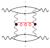
Figure 7: $s$-discontinuity for the scattering of two virtual photons with one additional real $s$-channel gluon. Wavy lines for $t$-channel gluons denote reggeized gluons.

which leads us to the diagram Fig.7. For the color factors on the cylinder we find, compared to the plane an important difference: in addition to the combinations that fits on the plane,

$$\parbox{56.9055pt}{\includegraphics[height=56.9055pt]{bfkl_1lopp_a.eps}}\qquad\to\qquad\parbox{85.35826pt}{ \includegraphics[width=71.13188pt]{cylinder_large_frontalt.eps}\quad,}$$ (29)

on the cylinder also the following combination contributes:

$$\parbox{85.35826pt}{\includegraphics[height=56.9055pt]{bfkl_1lopp_b.eps}}\qquad\to\qquad\parbox{99.58464pt}{ \includegraphics[width=71.13188pt]{cylinder_large_backalt.eps}\quad.}$$ (30)

For the two-to-two Reggeon transition on the cylinder we therefore obtain a factor two compared to the plane. This counting generalizes to diagrams with more than one real gluon: For each produced real gluon the two combinations of color factors Eq.(29) and Eq.(30) need to be added. An example with three produced gluons is shown in Fig.8:

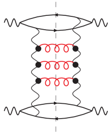
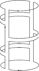
(a)

(b)

(c)

Figure 8: Multi-gluon emission within the MRK. (a) The cut Feynman diagram (b) Combination of relevant color diagrams of the production vertex. (c) The combination of (b) on the cylinder.

For each rung, we have two possibilities of connecting the $t$-channel lines of the ladder, either on the forefront and or on the backside of the cylinder Similar to the planar case discussed before, the summation over all production processes is done by formulating the BFKL equation on the cylinder. This integral equation coincides with Eq.(23), except for the factor $2$ in front of $K_{2\to 2}$, which results from the cylinder topology. Technically, we again split off the impact factor of the lower virtual photon and consider the partial wave amplitude $\mathcal{D}_{2}(\omega|{\bf k}_{1},{\bf k}_{2})$ for the scattering of a virtual photon on two reggeized gluons, which as before we define to contain the Reggeon propagator of the external reggeized gluons. We find

$$(\omega-\sum_{i}^{2}\beta({\bf{k}}_{i}))\mathcal{D}_{2}(\omega|{\bf k}_{1},{\bf k}_{2}) =\mathcal{D}_{2,0}({\bf k}_{1},{\bf k}_{2})+2\bar{\lambda}K_{2\to 2}\otimes\mathcal{D}_{2}(\omega|{\bf k}_{1},{\bf k}_{2}).$$ (31)

The kernel coincides with the BFKL kernel. Unlike the planar BFKL-equation Eq.(23), Eq.(31) has no pole solution, but the solution is known to have a cut in the complex $\omega$-plane. The solution is known both for the forward $(t=0)$ [3] and the non-forward $(t\neq 0)$ case [16]. Furthermore, the BFKL-Green’s function, which is obtained from $\mathcal{D}_{2}(\omega)$ by splitting up the impact factor of the above virtual photon, is invariant under Möbius transformations.

3 Six-point amplitudes and the pair-of-pants -topology

Returning to the expansion Eq.(6), we finally address the term with three boundaries and zero handles $b=3,h=0$. It is proportional to $1/N_{c}$ and leads to color factors that fit on the pair-of-pants, as illustrated in Fig.9. As we did for scattering amplitudes on the plane and on the cylinder, also for the pair-of-pants we identify a QCD-amplitude which, using the LLA, will be determined in a certain kinematical high energy limit.

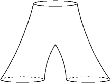
Figure 9: The sphere with three boundaries $b=3$ and no handles $h=0$ which yields the pair-of-pants.

As it was the case for the elastic amplitude, within the LLA, quark loops occur only inside the coupling to external states. In order to arrive at a surface with three boundaries, we are thus lead to a six-point amplitude, which we will study in the triple-Regge limit, to be specified in the following.

Within QCD, scattering amplitudes with more than $4$ external particles arise naturally in the context of deep inelastic scattering on a weakly bound nucleus, see Fig.10a.

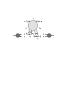
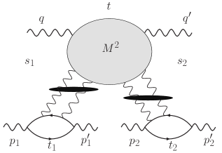
Figure 10: Scattering of a virtual photon on a weakly bound nucleus and the corresponding process where the lower nuclei are replaced by two highly virtual photons to the right.

To be definite, let us consider deep inelastic electron scattering on deuterium. The total cross section of this scattering process is obtained from the elastic scattering amplitude , $T_{\gamma^{*}(pn)\to\gamma^{*}(pn)}$, which describes a $3\to 3$ process,

$$\sigma^{tot}_{\gamma^{*}(pn)\to\gamma^{*}(pn)}=\frac{1}{s}\Im{\text{m}}\,T_{\gamma^{*}(pn)\to\gamma^{*}(pn)},$$ (32)

where $s$ denotes the square of the total center of mass energy of the scattering process. To study the pair-of-pants topology, we replace the two nucleons by virtual photons which furthermore provides us with a clean perturbative environment for the study of the six-point amplitude. The kinematics is illustrated in Fig.10. Large energy variables are $s_{1}=(q+p_{1})^{2}$, $s_{2}=(q^{\prime}+p^{\prime}_{2})^{2}$, and $M^{2}=(q+p_{1}-p^{\prime}_{1})^{2}$ which gives the squared mass of the diffractive system in which the upper virtual photon dissociates. The total energy square is given by $s=(q+p_{1}+p_{2})^{2}$. Furthermore, we have the momentum transfer variables $t=(q-q^{\prime})^{2}$, $t_{1}=(p_{1}-p^{\prime}_{1})^{2}$, and $t_{2}=(p_{2}-p^{\prime}_{2})^{2}$. The triple Regge-limit is given by $s_{1}=s_{2}\gg M^{2}\gg t,t_{1},t_{2}$. The investigation of such a process, for finite $N_{c}$, has been started in [7], in the context of diffractive dissociation in deep inelastic scattering, and in the following we will stay close to the methods used there.

Let us begin with finite $N_{c}$. The $3\to 3$ amplitude in the triple Regge limit has the following analytic representation

$$T_{3\to 3}(s_{1},s_{2},M^{2}|t_{1},t_{2},t)=\frac{s_{1}s_{2}}{M^{2}}\int\frac{d\omega_{1}d\omega_{2}d\omega}{(2\pi i)^{3}} s_{1}^{\omega_{1}}{s_{2}}^{\omega_{2}}(M^{2})^{\omega-\omega_{1}-\omega_{2}}\xi({\omega_{1}})\xi({\omega_{2}})\xi({\omega,\omega_{1},\omega_{2}})$$

$$\cdot F(\omega,\omega_{1},\omega_{2}|t,t_{1},t_{2}).$$ (33)

All three $t$-channels carry positive signature, and the signature factors are given by

$$\xi(\omega) =-\pi\frac{e^{-i\pi\omega}-1}{\sin(\pi\omega)} \xi({\omega,\omega_{1},\omega_{2}}) =-\pi\frac{e^{-i\pi(\omega-\omega_{1}-\omega_{2})}-1}{\sin\pi(\omega-\omega_{1}-\omega_{2})}.$$ and (34)

The partial wave $F(\omega_{1},\omega_{2},\omega|t_{1},t_{2},t)$ has no phases and is real valued. In analogy to the treatment of $T_{2\to 2}$, we take the triple energy discontinuity in $s_{1}$, $M^{2}$, and $s_{2}$,

$$\mathrm{disc}_{s_{1}}\mathrm{disc}_{s_{2}}\mathrm{disc}_{M^{2}}T_{3\to 3}=\pi^{3}\frac{s_{1}s_{2}}{M^{2}}\int\frac{d\omega_{1}d\omega_{2}d\omega}{(2\pi i)^{3}}s_{1}^{\omega_{1}}{s_{2}}^{\omega_{2}}(M^{2})^{\omega-\omega_{1}-\omega_{2}}\cdot F(\omega_{1},\omega_{2},\omega|t_{1},t_{2},t),$$ (35)

which via a triple Mellin transform relates the partial wave $F(\omega_{1},\omega_{2},\omega|t_{1},t_{2},t)$ to the real valued triple energy discontinuity.

Within the LLA, each of the three virtual photons couples to the $t$-channel gluons by a quark-loop (which in the topological expansion provides the three boundaries of the pair-of-pants). To leading order in $g^{2}$, four $t$ channel gluons couple to the upper quark-loop, and two gluons to each of the two lower quark-loops, which yields diagrams like the one shown in Fig.11.

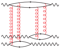
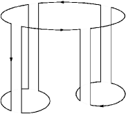
Figure 11: An example of a leading order diagram for the six-point amplitude with its color factor depicted to the right. The diagram is proportional to $g^{8}N_{c}^{3}=\lambda^{4}N_{c}^{-1}$ as required for the pair-of-pants.

When taking the triple energy discontinuity, all intermediate states between the $t$ channel gluons are on mass-shell. For higher order corrections to these diagrams, we make extensive use of unitarity and compute sums over products of production processes. Some examples are shown in Fig.12.

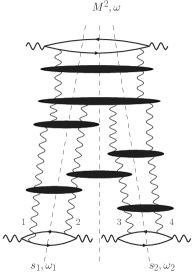
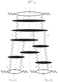
Figure 12: A few contributions to the triple energy discontinuity of Eq.(33)

Due to the triple discontinuity, $t$-channel gluons do not intersect, and it is therefore useful to enumerate them from the left to right, with the most left gluon carrying the index $1$. In order to form, within the LLA, color singlet states which at the top couple to the virtual photon and at the bottom to two virtual photons, we are lead to QCD diagrams with four $t$-channel gluons at the lower and two, three or four $t$-channel gluons at the upper end. In contrast to our previous discussion of scattering processes on the plane and on the cylinder, the number of $t$-channel gluons can change, i.e. a $t$ channel gluon can emerge also from a $s$ channel produced gluon. However, in LLA there is the restriction that, when moving downwards, the number of reggeized $t$ channel gluons never decreases.

A special role in our analysis is taken by the diffractive mass $M^{2}$ as it defines the size of the upper ’cylinder’ of the pair-of-pants. In particular, the lowest intermediate state inside the $M^{2}$-discontinuity (descending from the top to the bottom of the diagram) defines the last interaction between the two ’legs’ of the pants, i.e. the branching point of the upper into the two lower cylinders. We use this branching point to factorize the partial wave $F(\omega,\omega_{1},\omega_{2})$ into a convolution of three different amplitudes. With $s_{1},s_{2}\gg M^{2}\gg t,t_{1},t_{2}$, the diagrams below the branching point, within the LLA, do not depend on the details of the dissociation of the upper virtual photon, and are therefore described by two independent amplitudes $\mathcal{D}_{2}(\omega_{1})$ and $\mathcal{D}_{2}(\omega_{2})$ which describe scattering of two $t$-channel gluons and their coupling to the lower photons. The functions $\mathcal{D}_{2}(\omega_{1})$ and $\mathcal{D}_{2}(\omega_{2})$ are given by BFKL-Pomeron Green’s functions, convoluted with the impact factors of the corresponding lower virtual photon. In the following we will confirm that, in our topological approach, on the pair-of-pants the required color factors work out correctly. The part above the the branching point is resummed by the amplitude $\mathcal{D}_{4}(\omega)$, which describes the scattering of the upper virtual photon on the four $t$-channel gluons. In the following, our interest will mainly concentrate on this part of our scattering amplitude.

4 Color factors with pair-of-pants topology

After our general outline of which QCD diagrams contribute to the leading log approximation of the $3\to 3$ process we have to select now the contributions which belong to the large-$N_{c}$ limit on the pair-of-pants. This will be done by attributing to each QCD diagram a ’color diagram’ on the pair-of pants surface, where each gluon is drawn by a pair of color lines with opposite directions, as done for the plane and the cylinder in Sec.2.

4.1 Color factors at Born-level

All diagrams that contribute to the Born approximation of the triple-discontinuity have the form of Fig.11, with $t$-channel gluons coupling to the the quark-loop in all possible ways. Overall, one finds sixteen different diagrams. Because of the triple energy discontinuity $t$-channel gluons never intersect and hence can be labeled from the left to the right. A closer look then shows that, inside the quark loop, we have the four different orderings of color matrices: (1234), (2134), (1243), and (2143) (not distinguishing between cyclic permutations ). These four structures are illustrated in Fig.13

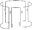
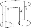
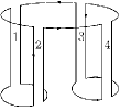
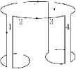
$(1234)$

${(2134)}$

${(1243)}$

${(2143)}$

Figure 13: The four different orderings of color factors of the Born-term.

and are all of the order

$$g^{8}N_{c}^{3}=N_{c}^{-1}\lambda^{4}.$$ (36)

4.2 Gluon production on the pair-of-pants surface

In order to study corrections to these Born-amplitudes, we consider real gluon production processes on the pair-of-pants surface ($t$-channel gluons are always reggeized). As to the selection of diagrams, we are searching the maximal power of color factors $N_{c}$. With (36) the diagrams we are going to collect will come with the weight

$$g^{8}N_{c}^{3}(g^{2}N_{c})^{k}=N_{c}^{-1}\lambda^{4+k},$$ (37)

with $k$ being some positive integer number. This leads to the requirement that, for each gluon, the pair of color lines has to be planar, i.e. it never intersects.

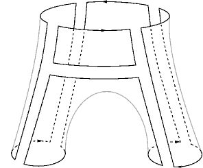
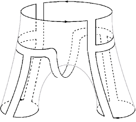
(a)

(b)

Figure 14: (a) A typical color factor of the planar class (A). (b) A typical color factor of the non-planar class (B) which has the interpretation of the Mandelstam diagram.

As a result we find two classes of color diagrams. The first class (A) consists of all diagrams which, by contracting closed color loops, coincide with one of the lowest order diagrams in Fig.13. An example for such a diagram is given in Fig.14.a. In the following we will refer to these diagrams as ’planar’ diagrams. The second class (B) consists of those diagrams where the ’last’ vertex before the separation into the two lower cylinders is of the form illustrated in Fig.14.b: one easily verifies that the power of color factors is $g^{8}N_{c}^{3}(g^{2}N_{c})=N_{c}^{-1}\lambda^{4+1}$, as required by condition Eq.(37). Also, there is no intersection of color lines on the pair-of-pants surface. These diagrams cannot be redrawn, by contracting closed color loops in a straightforward way, such that they coincide with one of the lowest order diagrams of Fig.13. The structure shown in Fig.14.b is reminiscent of the Mandelstam diagram (’Mandelstam cross’) which, when integrated over the diffractive mass $M$, couples to the two Pomeron cut; we will therefore call it ’non-planar’ (although it fits onto the surface of the pair-of-pants). Note that this non-planar structure appears only once, namely at the point where the upper cylinder splits into the two lower ones.

In the remainder of this section, we describe these two sets of diagrams in more detail. In particular, we list the momentum space expressions which belong to the gluon transition kernels. In the following section, we derive integral equations which sum all diagrams of set (A). For set (B) we re-derive the triple Pomeron vertex.

4.3 Two-to-two Reggeon transitions

We start with the case, where all four $t$-channel gluons couple to the upper quark-loop. We therefore consider only insertions of the two-to-two transition kernel,

$$\parbox{56.9055pt}{\includegraphics[width=42.67912pt]{k22_cut.eps}}=\bar{g}^{2}\big{(}\parbox{14.22636pt}{\includegraphics[width=14.22636pt]{structure1.eps}}-\parbox{14.22636pt}{\includegraphics[width=14.22636pt]{structure2.eps}}\big{)}\cdot\big{(}\parbox{14.22636pt}{\includegraphics[width=14.22636pt]{structure2.eps}}-\parbox{14.22636pt}{\includegraphics[width=14.22636pt]{structure1.eps}}\big{)}K_{2\to 2}({\bf l}_{1},{\bf l}_{2};{\bf k}_{1},{\bf k}_{2}),$$ (38)

into the Born diagrams of Fig.13, with $K_{2\to 2}$ given by Eq.(22). To be definite, we consider corrections to the first diagram of Fig.13; the other Born diagrams are treated in the same way. We start with the case where the interaction is between gluons which end up in the same lower quark-loop, i.e. the interaction is inside the gluon pairs (12) or (34). In the case of the gluon pair (12), the two combinations of color factors of Fig.15 fit on the pair-of-pants,

Figure 15: Two combination of color-factors for the interaction between gluons ’1’ and ’2’.

similar to the cylinder discussed before. An analogous result holds for the gluon pair (34). If the interacting $t$-channel gluons end up in different quark-loops we need to distinguish between two different cases. In the first case, shown in Fig.16, the interaction is between gluons ’2’ and ’3’; on the surface of the upper cylinder the two gluons are neighboring.

Figure 16: Color-factors of an interacting between two neighboring $t$-channel gluons.

We call this interaction planar: by contracting the color loop above the rung between gluon ’2’ and ’3’, we are back to the first Born diagram in Fig.13. In the second case, shown in Fig.17, the interaction is between gluon ’2’ and ’4’, These two gluons are not neighboring, and although the color diagram fits onto the surface of the pair-of-pants without any intersection of color lines, it will be referred to as ’non-planar’. It cannot be reduced to the Born diagram in Fig.13. Counting closed color loops, it is of the same order as that of Fig.16.

Figure 17: Color factors of an interaction between two non-neighboring $t$-channel gluons.

Note, however, that compared to the planar one it has a relative minus sign. The same discussion applies if the interaction is between gluon ’1’ and ’3’.

We summarize the four possibilities in Fig.18.

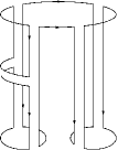
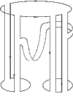
(a)

(b)

(c)

(d)

Figure 18: Different structures due to insertion of a two-to-two kernel on the pair-of-pants.

Apart form the last diagram, all diagrams belong to the class of ’planar’ graphs. Note, however, that while in the first graph we can contract the closed color loop either above or below, in the second graph we can contract only the lower loop on the lower cylinder: it is planar w.r.t. the lower left cylinder.

When inserting more two-to-two interactions, it is useful to descend from the top to the bottom of the diagram: we start by inserting $s$-channel gluons between $t$-channel gluons which, on the upper cylinder, are neighboring (Figs.18a and c). This generates planar graphs. Moving further down, these planar insertions come to a stop as soon as one of the following interactions is included:
(i) either an interaction of the type Fig.18b which is still planar but belongs to the lower left cylinder. Below such an interactions, further interactions lie on the surface of one of the two lower cylinders, i.e. they are inside the pairs $(12)$ or $(34)$. An interaction between the two cylinders, e.g., between gluon ’1’ and ’3’, loses a color factor $N_{c}$ and does not contribute on the pair-of-pants.
(ii) alternatively, a non-planar interaction of the type Fig.18: This interaction occurs at most once, and any further interaction below, again, lies on the surface of one of the two lower cylinders and hence is inside the pairs $(12)$ or $(34)$.

4.4 Two-to-four Reggeon transition

Apart from the above examples we have further the possibility that some of the $t$-channel gluons do not start at the upper quark loop but emerge from produced $s$-channel gluons. We start with the transition from two to four $t$-channel gluons. In this case we start, at the upper quark loop, with two $t$-channel gluons which end at a two-to-four transition. Leaving for the moment details on the momentum structure of the transition kernel $K_{2\to 4}$ aside, the transition from two to four reggeized gluons is given by

$$\parbox{56.9055pt}{\includegraphics[height=28.45274pt]{k24_cut.eps}}={\bar{g}}^{4}\bigg{(}\parbox{14.22636pt}{\includegraphics[width=14.22636pt]{structure1.eps}}-\parbox{14.22636pt}{\includegraphics[width=14.22636pt]{structure2.eps}}\bigg{)}\bigg{(}\parbox{31.2982pt}{\includegraphics[height=14.22636pt]{structure4.eps}}-\parbox{31.2982pt}{\includegraphics[height=14.22636pt]{structure3.eps}}\bigg{)}\bigg{(}\parbox{31.2982pt}{\includegraphics[height=14.22636pt]{structure4.eps}}-\parbox{31.2982pt}{\includegraphics[height=14.22636pt]{structure3.eps}}\bigg{)}\bigg{(}\parbox{14.22636pt}{\includegraphics[width=14.22636pt]{structure2.eps}}-\parbox{14.22636pt}{\includegraphics[width=14.22636pt]{structure1.eps}}\bigg{)}K_{2\to 4}.$$ (39)

Of the 16 possible combinations of color factors, only a subset fits on the pair-of-pants, of which two examples are shown in Figs.19 and 20.

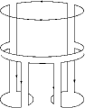
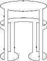
Figure 19: The planar two-to-four Reggeon transition.

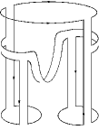
Figure 20: The non-planar two-to-four Reggeon transition.

Again, we have two distinct structures: Fig.19, by contracting the closed color loop on the upper cylinder, can be reduced to one of the Born diagrams, and thus belongs to class of planar diagrams. In contrast, Fig.20 cannot be contracted and is non-planar.

Further rungs above the $2\to 4$ transition vertex can always be contracted to either Figs.19 or 20. As to the interactions below the $2\to 4$ transition, we have to distinguish between the two classes. For the planar class in Figs.19, we can continue by inserting $2\to 2$ interactions as described in the previous subsection. For the non-planar class in Fig.20 any further $2\to 2$ interaction is either inside the pair $(12)$ or $(34)$ and can always be reduced to Fig.20.

For the momentum structure of the $2\to 4$ transition vertex we need, apart from the real gluon production vertex in Eq.(19), the vertex which describes coupling of a $t$-channel gluon to a real $s$-channel gluon, which is known as the Reggeon-Particle-Particle (RPP)-vertex. Similar to the production vertex, the RPP-vertex is an effective vertex. To lowest order, for the scattering of a gluon on an antiquark at high center of mass energies, this RPP-vertex is built up from the following diagrams:

$$\parbox{42.67912pt}{\includegraphics[width=42.67912pt]{fadin.eps}}=\parbox{42.67912pt}{\includegraphics[width=42.67912pt]{fadin1.eps}}+\parbox{42.67912pt}{\includegraphics[width=42.67912pt]{fadin3.eps}}+\parbox{42.67912pt}{\includegraphics[width=42.67912pt]{fadin2.eps}.}$$ (40)

Similar to the production vertex, at high center of mass energies the last two diagrams coincide with each other up to a sign, and color factor and momentum part of the RPP-vertex can be written in the factorized form

$$-i{\bar{g}}\left[\parbox{42.67912pt}{\includegraphics[width=42.67912pt]{structure4.eps}}-\parbox{42.67912pt}{\includegraphics[width=42.67912pt]{structure3.eps}}\right]\epsilon^{*}_{(\lambda^{\prime})}\!\!\cdot\!\Gamma\!\cdot\!\epsilon_{(\lambda)}.$$ (41)

Sandwiching one or two RPP vertices between two production vertices then leads to two-to-three and two-to-four Reggeon transition kernels. They have been constructed in [5] and for details we refer to this reference. The momentum part of the the $2\to 4$ transition is then given by

$$K_{2\to 4}={\bf q}^{2} -\frac{{\bf l}_{1}^{2}({\bf q}-{\bf k}_{1})^{2}}{({\bf l}_{1}-{\bf k}_{1})^{2}}-\frac{{\bf l}_{2}^{2}({\bf k}_{1}+{\bf k}_{2}+{\bf k}_{3})^{2}}{({\bf l}_{2}-{\bf k}_{4})^{2}}+\frac{{\bf l}_{1}^{2}({\bf q}-{\bf k}_{1})^{2}{\bf l}^{2}_{2}}{({\bf l}_{1}-{\bf k}_{1})^{2}({\bf l}_{2}-{\bf k}_{4})^{2}}.$$ (42)

4.5 Two-to-three Reggeon transition

Last we need to consider diagrams that contain, at least, one transition from two to three gluons. Beginning with the momentum structure, we remind that the coupling of an additional ’new’ $t$-channel to an $s$-channel gluon takes place by the RPP-vertex in Eq.(41). The result for two-to-three Reggeon transition is described by

$$\parbox{56.9055pt}{\includegraphics[height=28.45274pt]{k23_cut.eps}}=i\bar{g}^{3}\bigg{(}\parbox{14.22636pt}{\includegraphics[width=14.22636pt]{structure1.eps}}-\parbox{14.22636pt}{\includegraphics[width=14.22636pt]{structure2.eps}}\bigg{)}\bigg{(}\parbox{31.2982pt}{\includegraphics[height=14.22636pt]{structure4.eps}}-\parbox{31.2982pt}{\includegraphics[height=14.22636pt]{structure3.eps}}\bigg{)}\bigg{(}\parbox{14.22636pt}{\includegraphics[width=14.22636pt]{structure2.eps}}-\parbox{14.22636pt}{\includegraphics[width=14.22636pt]{structure1.eps}}\bigg{)}K_{2\to 3}$$ (43)

with

$$K_{2\to 3}^{(\{12\}\to\{123\})}=({\bf k}_{1}+{\bf k}_{2}+{\bf k}_{3})^{2} -\frac{{\bf l}_{1}^{2}({\bf k}_{2}+{\bf k}_{3})^{2}}{({\bf l}_{1}-{\bf k}_{1})^{2}}-\frac{{\bf l}_{2}^{2}({\bf k}_{1}+{\bf k}_{2})^{2}}{({\bf l}_{2}-{\bf k}_{3})^{2}}+\frac{{\bf l}_{1}^{2}{\bf k}_{2}^{2}{\bf l}^{2}_{2}}{({\bf l}_{1}-{\bf k}_{1})^{2}({\bf l}_{2}-{\bf k}_{3})^{2}},$$ (44)

where the superscripts on the kernel refer to the ingoing and outgoing $t$-channel gluons respectively. As to the general structure of diagrams with $2\to 3$ transitions, we have two possibilities: either we start, at the upper quark loop, with three gluons. In this case we need, somewhere further below, only one $2\to 3$ transition. Alternatively, we could start with two gluons and then need two $2\to 3$ transition vertices.

For the discussion of the color diagrams we start with the former case. As before we encounter planar and non-planar graphs. An example of a planar graph is shown in Fig.21, a non-planar graph in Fig.22. In both cases, the planar class, Fig.21,

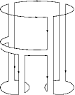
Figure 21: Planar graph with one two-to-three transition.

and the non-planar class, Fig.22,

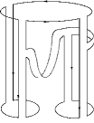
Figure 22: Non-planar graph with one two-to-three transition.

above the vertex any further $2\to 2$ interaction is between lines which are neighbored on the surface of the upper cylinder. Below the $2\to 3$ vertex we have the same situation as for the $2\to 4$ vertex: for the planar graph in Fig.21 we proceed as described in Sec.4.3, whereas for the non-planar graph there is no further communication between the two lower cylinders.

For the graphs which, at the top, start with two $t$-channel gluons the two classes arise in the following way. Beginning at the top, the first $2\to 3$ transition always lies on the surface of the upper cylinder. Below this vertex we have the same situation which we have described a moment ago, i.e. the same as for the case where at the fermion quark loop we start with three gluons: the second $2\to 3$ transition decides whether the graph is planar or non-planar. Planar examples are shown in Fig.23.

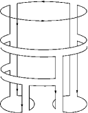
Figure 23: Combination of two transitions of two to three $t$-channel gluons. From Eq.(43) one finds a relative minus sign for the second combination.

4.6 Planar and non-planar partial waves

In this final subsection we collect the results and prepare the summation of all diagrams on the pair-of-pants surface. At the end of Sec.3 we proposed to factorize at the branching point, i.e. at the last interaction between the two ’legs’ of the pair-of-pants, the partial wave $F(\omega,\omega_{1},\omega_{2})$ into a convolution of three amplitudes $\mathcal{D}_{4}(\omega)$, $\mathcal{D}_{2}(\omega_{1})$, and $\mathcal{D}_{2}(\omega_{2})$, depending on $\omega$, $\omega_{1}$, or $\omega_{2}$, resp.. In order to find closed expressions for these amplitudes we shall, similar to our treatment of the diagrams in the plane and on the surface of the cylinder, formulate integral equations which sum up the different classes of diagrams.

The situation is easiest for the two amplitudes that start from the two lower virtual photons, $\mathcal{D}_{2}(\omega_{1})$, and $\mathcal{D}_{2}(\omega_{2})$. For these amplitudes we need to resum, for both legs, contributions like those in Fig.15. Their resummation yields the BFKL-equation on the cylinder Eq.(31).

The upper amplitude, $\mathcal{D}_{4}(\omega)$ is defined to include the branching vertex, which by definition is the lowest interaction that connects the gluon pair (12) with the pair (34). Below this vertex, there are only interactions inside the pair $(12)$ or $(34)$. The branching vertex can be either a $2\to 2$, a $2\to 3$, or a $2\to 4$ transition vertex. From this definition it follows that the upper amplitude always has four reggeized gluons at its lower end.

From now on it becomes important to distinguish between ’planar’ and ’non-planar’ graphs.

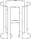
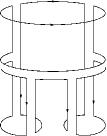
(a)

(b)

(c)

Figure 24: ’Planar’ color factors on the pair-of-pants which reduce in an apparent way to the color structure of the Born-term by extracting a closed color loop with the upper quark-loop.

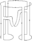
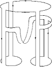
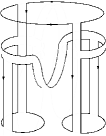
(a)

(b)

(c)

Figure 25: ’Non-planar’ color factors that cannot be reduced trivially to the color structure of the Born-term by extracting a closed color loop with the upper quark-loop.

For convenience we list, once more, three examples of planar and non-planar graphs: Fig.24 contains the planar example, and Fig.25 the non-planar ones. They are of the order $g^{8}N_{c}^{3}(g^{2}N_{c})$.

Beginning with the planar diagrams in Fig.24 one easily verifies that we always can contract one closed color loop to arrive at the first diagram of Fig.13. For the other diagrams in Fig.13 we have analogous sets of graphs. Next, the figures Fig.24a-c differ from each other in that, at the fermion loop at the top, in (a) we start with four gluons, in (b) with only three gluons, and in (c) with two gluons. Correspondingly, in (a) the branching vertex consists of a two-to-to kernel, in (b) a two-to-three kernel, and in (c) a two-to-four kernel. At the branching vertex, all diagrams have four $t$-channel gluon lines. Higher order diagrams are obtained by inserting, above the branching vertex, pairwise interactions between neighboring $t$-channel gluons. Also, in Fig.24b and d we could insert a $2\to 2$ interaction between gluons ’2’ and ’3’ or ’1’ and ’4’: in this case, the branching vertex consists of a two-to-to kernel. In all cases, by drawing a horizontal cutting line just below the branching vertex, we arrive at amplitudes with four $t$-channel gluons. We will denote the sum of all graphs by $\mathcal{D}_{4}^{(1234)}(\omega)$, $\mathcal{D}_{4}^{(2134)}(\omega)$, $\mathcal{D}_{4}^{(2143)}(\omega)$, and $\mathcal{D}_{4}^{(2134)}(\omega)$ where the upper label refers to the four terms in Fig.13, i.e. it indicates to which of the four Born terms the diagrams can be contracted (a more precise definition will be given further below in section 5).

For the task of summing of all diagrams it will be convenient to define also auxiliary amplitudes with two and three gluons in the $t$-channel. In Fig.24c one sees that, starting at the upper quark loop, we begin with two gluons which, when higher order corrections are included, interact through two-to-two kernels. The sum of these diagrams leads to the BFKL cylinder and therefore coincides with $\mathcal{D}_{2}(\omega)$ of Sec.2.3.

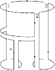
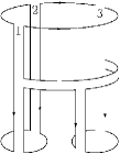
${(123)}$

${(321)}$

Figure 26: The two possible orderings of three gluons along the quark-loop which leads to the definition of $\mathcal{D}_{3}^{(123)}(\omega)$ and $\mathcal{D}_{3}^{(321)}(\omega)$.

For the three gluon amplitude above the branching vertex in Fig.24b we have two inequivalent couplings to the quark loops, as illustrated in Fig.26. We denote them by $\mathcal{D}_{3}^{(123)}(\omega)$ and $\mathcal{D}_{3}^{(132)}(\omega)$.

When writing down integral equations for the amplitudes $\mathcal{D}_{3}$ and $\mathcal{D}_{4}$, we observe that they will be coupled. The three gluon state at the lower end of $\mathcal{D}_{3}$ can start as a two gluons at the quark loop, then undergo a two-to-three transition. Similarly, the four gluon state can start from two or three gluons and then make transitions to the final four gluon state. The formulation of these coupled integral equations will be carried out in the subsequent section.

Next we turn to the non-planar diagrams of Fig.25. They cannot be reduced to the color structure of the Born diagrams, and we therefore define an additional partial wave that sums up these terms. They all have in common that the non-planar structure at the lower end of the upper cylinder is always the branching vertex: below this vertex, there is no further communication between the two lower cylinders. As an example, an interaction between gluon ’2’ and ’3’ would be subleading in powers $N_{c}$. Similar to the planar diagrams in Fig.24, we see three different structures: above the branching vertex we have four (Fig.24a), three (Fig.24b), or two (Fig.24c) $t$-channel gluons. This suggests that above the branching vertex the structure is the same as for the planar graphs, and we simply have to convolute the non-planar branching vertex with the planar amplitudes $\mathcal{D}_{2}$, $\mathcal{D}_{3}$, and $\mathcal{D}_{4}$. The resulting expression will be denoted by $\mathcal{D}_{4}^{(\text{NP})}(\omega)$. Its derivation will be the content of Sec.6.

5 Integral equations: gluon amplitudes with planar color structure

In the following we will formulate integral equations for amplitudes of the planar class with two, three and four $t$-channel gluons. The amplitude with four $t$-channel gluons that belongs to the non-planar class will be addressed in Sec.6.

5.1 Integral equations for the three gluon amplitude

The evolution of the three gluon state is described by the sum of pairwise interactions, i.e. the two-to-two transition kernels acting on the three gluon state

$$\parbox{56.9055pt}{\includegraphics[width=56.9055pt]{ql3_k22_12.ps}}+\parbox{65.44142pt}{\includegraphics[width=56.9055pt]{ql3_k22_23.ps}}+\,\parbox{56.9055pt}{\includegraphics[width=56.9055pt]{ql3_k22_31.ps}}\to\bar{g}^{2}N_{c}\sum_{\begin{subarray}{c}(12),(23)\\ (31)\end{subarray}}K_{2\to 2}\otimes\mathcal{D}_{3}^{(123)}(\omega).$$ (45)

The transition from the two gluon state to the three gluon state is mediated by the two-to-three transition kernels acting on the two-gluon state,

$$\parbox{71.13188pt}{\includegraphics[width=71.13188pt]{two3a_num.ps}}\to{\bar{g}^{3}}(-N_{c})K_{2\to 3}^{(\{12\}\to\{123\})}\otimes\mathcal{D}_{2}(\omega).$$ (46)

Similar to $\mathcal{D}_{2}(\omega)$, also the amplitude $\mathcal{D}_{3}(\omega)$ is defined to contain the Reggeon propagator of the external reggeized gluons, $1/(\omega-\sum_{i}^{3}\beta({\bf k}_{i}))$. With these ingredients, the integral equation for $\mathcal{D}_{3}^{(123)}(\omega)$ is given by

$$\big{(}\omega-\sum_{i}^{3}\beta({\bf{k}}_{i})\big{)}\mathcal{D}_{3}^{(123)}(\omega|{\bf k}_{1},{\bf k}_{2},{\bf k}_{3})= \mathcal{D}^{(123)}_{(3,0)}+{\bar{g}}^{3}(-N_{c})K^{(\{12\}\to\{123\})}_{2\to 3}\otimes\mathcal{D}_{2}(\omega)$$

$$+\bar{g}^{2}N_{c}\sum K_{2\to 2}\otimes\mathcal{D}^{(123)}_{3}(\omega).$$ (47)

In complete analogy the equation for $\mathcal{D}_{3}^{(321)}(\omega)$ contains the two-to-three transition kernel

$$\parbox{71.13188pt}{\includegraphics[width=71.13188pt]{two3b_num.ps}}\to{\bar{g}}^{3}N_{c}K_{2\to 3}^{(\{12\}\to\{123\})}\otimes\mathcal{D}_{2}(\omega).$$ (48)

The integral equation is given by:

$$\big{(}(\omega-\sum_{i}^{3}\beta({\bf{k}}_{i})\big{)}\mathcal{D}_{3}^{(321)}(\omega|{\bf k}_{1},{\bf k}_{2},{\bf k}_{3})= \mathcal{D}^{(321)}_{(3,0)}+\bar{g}^{3}N_{c}K^{(\{12\}\to\{123\})}_{2\to 3}\otimes\mathcal{D}_{2}(\omega)$$

$$+\bar{g}^{2}N_{c}\sum_{\begin{subarray}{c}(13),(32)\\ (21)\end{subarray}}K_{2\to 2}\otimes\mathcal{D}^{(321)}_{3}(\omega).$$ (49)

5.2 Reggeization of the three-gluon amplitude

To study the integral equations Eq.(5.1) and Eq.(5.1) we need the impact factors $\mathcal{D}_{(3;0)}^{(123)}$ and $\mathcal{D}_{(3;0)}^{(321)}$. Both impact factors have the same properties as in the $N_{c}$ finite case [7], and they can be written as a superposition of two-gluon impact factors $\mathcal{D}_{(2;0)}$:

$$\mathcal{D}_{(3;0)}^{(123)}({\bf k}_{1},{\bf k}_{2},{\bf k}_{3}) =+\frac{{\bar{g}}}{2}\big{[}\mathcal{D}_{(2;0)}(12,3)-\mathcal{D}_{(2;0)}(13,2)+\mathcal{D}_{(2;0)}(1,23)\big{]}$$ (50)

$$D_{(3;0)}^{(321)}({\bf k}_{1},{\bf k}_{2},{\bf k}_{3}) =-\frac{{\bar{g}}}{2}\big{[}D_{(2;0)}(12,3)-D_{(2;0)}(13,2)+D_{(2;0)}(1,23)\big{]}.$$ (51)

On the right hand side we introduced a short-hand notation: a string of numbers stands for the sum of the corresponding transverse momenta, for instance

$$\mathcal{D}_{(2;0)}(12,3)\equiv\mathcal{D}_{(2;0)}({\bf k}_{1}+{\bf k}_{2},{\bf k}_{3}).$$ (52)

We will make use of this notation in the following, whenever it proves useful to clarify the underlying structure of complex expressions. It can be now demonstrated that the structure on the rhs of Eqs.(50] and Eqs.(51 also holds for the solutions of the integral equations Eq.(5.1) and Eq.(5.1):

$$\mathcal{D}_{3}^{(123)}(\omega|{\bf k}_{1},{\bf k}_{2},{\bf k}_{3})=+\frac{{\bar{g}}}{2}\big{[}\mathcal{D}_{2}(\omega|12,3)-\mathcal{D}_{2}(\omega|13,2)+\mathcal{D}_{2}(\omega|1,23)\big{]}$$ (53)

$$\mathcal{D}_{3}^{(321)}(\omega|{\bf k}_{1},{\bf k}_{2},{\bf k}_{3})=-\frac{{\bar{g}}}{2}\big{[}\mathcal{D}_{2}(\omega|12,3)-\mathcal{D}_{2}(\omega|13,2)+\mathcal{D}_{2}(\omega|1,23)\big{]}.$$ (54)

Obviously this solution shares important properties with the reggeization of the planar gluon discussed in Sec.2.2: in each term on the rhs, two gluons ’collapse’ into a single gluon which, at the end, decays into two gluons. This allows also to deform the color factor as shown in Fig.27:

= = =

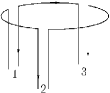
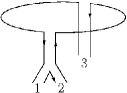
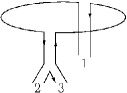
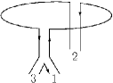
Figure 27: The color factor associated with $\mathcal{D}_{3}^{(123)}(\omega)$ can be deformed such that the form of the color factor coincides with the momentum structure of the solution in terms of $\mathcal{D}_{2}$. A similar observation holds for $\mathcal{D}_{3}^{(321)}(\omega)$.

5.3 The integral equations for the four gluon amplitude with planar color structure

For the four gluon amplitude, $\mathcal{D}_{4}^{(1234)}(\omega)$, the evolution of the four gluon state is describes by the sum of pairwise interactions between neighboring gluons. For the amplitude $\mathcal{D}_{4}^{(1234)}(\omega)$ the sum of the two-to-two transition is given by

$$\parbox{56.9055pt}{ \includegraphics[width=56.9055pt]{ql1234_k22_12.ps}}+\parbox{56.9055pt}{ \includegraphics[width=56.9055pt]{ql1234_k22_23.ps}}+\parbox{56.9055pt}{ \includegraphics[width=56.9055pt]{ql1234_k22_34.ps}}+\parbox{56.9055pt}{ \includegraphics[width=56.9055pt]{ql1234_k22_41.ps}}\to\bar{g}^{2}N_{c}\sum_{\begin{subarray}{c}(12),(23)\\ (34),(41)\end{subarray}}K_{2\to 2}\otimes\mathcal{D}_{4}^{(1234)}(\omega).$$ (55)

The corresponding expressions for $\mathcal{D}_{4}^{(2134)}(\omega)$, $\mathcal{D}_{4}^{(2143)}(\omega)$ and $\mathcal{D}_{4}^{(1243)}(\omega)$ are easily obtained by simply exchanging the corresponding labels on the $t$-channel gluons. For $\mathcal{D}_{4}^{(1234)}(\omega)$, the two-to-three transitions are

$$\parbox{56.9055pt}{ \includegraphics[width=56.9055pt]{trouser3a_inta1234.ps}}+\parbox{56.9055pt}{ \includegraphics[width=56.9055pt]{trouser3b_inta1234.ps}}\quad\to\begin{array}[]{l}\bar{g}^{3}N_{c}K_{2\to 3}^{(\{12\}\to\{123\})}\otimes D_{3}^{(123)}(\omega)\\ \\ +\quad\bar{g}^{3}N_{c}K_{2\to 3}^{(\{23\}\to\{234\})}\otimes D_{3}^{(123)}(\omega),\end{array}$$ (59)

while the two-to-four transition is

$$\parbox{56.9055pt}{ \includegraphics[width=56.9055pt]{two4_1_num.ps}}\quad\to\bar{g}^{4}{N_{c}}K_{2\to 4}^{(\{12\}\to\{1234\})}\otimes\mathcal{D}_{2}(\omega).$$ (60)

Also $\mathcal{D}_{4}^{(1234)}(\omega)$ is defined to contain the Reggeon-propagator of the external reggeized gluons. Including this contribution together with the four gluon impact factor, $\mathcal{D}_{(4;0)}^{(1234)}$, the integral equation for $\mathcal{D}_{4}^{(1234)}(\omega)$ is given by

$$(\omega-\sum_{i}^{4}\beta({\bf k}_{i}))\mathcal{D}_{4}^{(1234)}(\omega) =\mathcal{D}^{(1234)}_{(4;0)}+{\bar{g}}^{3}N_{c}\bigg{[}K_{2\to 3}^{(\{12\}\to\{123\})}\!\!\otimes\!\mathcal{D}_{3}^{(123)}(\omega)+K_{2\to 3}^{(\{23\}\to\{234\})}\!\!\otimes\!\mathcal{D}_{3}^{(123)}(\omega)\bigg{]}$$

$$+{\bar{g}^{4}}{N_{c}}^{2}K_{2\to 4}^{(\{12\}\to\{1234\})}\otimes\mathcal{D}_{2}(\omega)+\bar{g}^{2}N_{c}\sum_{\begin{subarray}{c}(12),(23)\\ (34),(41)\end{subarray}}K_{2\to 2}\otimes\mathcal{D}_{4}^{(1234)}(\omega).$$ (61)

For $\mathcal{D}_{4}^{(2143)}(\omega)$ the two-to-three transition arises from

$$\parbox{56.9055pt}{ \includegraphics[width=56.9055pt]{trouser3a_inta2143.ps}}+\parbox{56.9055pt}{ \includegraphics[width=56.9055pt]{trouser3b_inta2143.ps}}\quad\to\begin{array}[]{l}\\ {\bar{g}}^{3}(-N_{c})K_{2\to 3}^{(\{12\}\to\{123\})}\otimes\mathcal{D}_{3}^{(321)}(\omega)\\ \\ +\quad{\bar{g}}^{3}(-N_{c})K_{2\to 3}^{(\{23\}\to\{234\})}\otimes\mathcal{D}_{3}^{(321)}(\omega),\end{array}$$ (66)

and the two-to-four transition comes from

$$\parbox{56.9055pt}{ \includegraphics[width=56.9055pt]{two4_2_num.ps}}\quad\to{\bar{g}^{4}}{N_{c}}K_{2\to 4}^{(\{12\}\to\{1234\})}\otimes\mathcal{D}_{2}(\omega).$$ (67)

We obtain the integral equation

$$(\omega-\sum_{i}^{4}\beta({\bf k}_{i}))\mathcal{D}_{4}^{(2143)}(\omega) =\mathcal{D}^{(2143)}_{(4;0)}+{\bar{g}}^{3}(\!-\!N_{c})\bigg{[}K_{2\to 3}^{(\{12\}\!\to\!\{123\})}\!\!\otimes\!\mathcal{D}_{3}^{(321)}(\omega)+K_{2\to 3}^{(\{23\}\!\to\!\{234\})}\!\!\otimes\!\mathcal{D}_{3}^{(321)}(\omega)\bigg{]}$$

$$+{\bar{g}^{4}}{N_{c}}^{2}K_{2\to 4}^{(\{12\}\to\{1234\})}\otimes\mathcal{D}_{2}(\omega)+\bar{g}^{2}\sum_{\begin{subarray}{c}(21),(14)\\ (43),(32)\end{subarray}}K_{2\to 2}\otimes\mathcal{D}_{4}^{(2143)}(\omega)$$ (68)

Finally, for $\mathcal{D}_{4}^{(2134)}(\omega)$ and $\mathcal{D}_{4}^{(1243)}(\omega)$ the two-to-three transition are

$$\parbox{56.9055pt}{ \includegraphics[width=56.9055pt]{trouser3b_inta2134.ps}}+\parbox{56.9055pt}{ \includegraphics[width=56.9055pt]{trouser3a_inta2134.ps}}\quad\to\begin{array}[]{l}\bar{g}^{3}(-N_{c})K_{2\to 3}^{(\{13\}\to\{124\})}\otimes\mathcal{D}_{3}^{(123)}(\omega)\\ \\ +\quad{\bar{g}}^{3}N_{c}K_{2\to 3}^{(\{13\}\to\{134\})}\otimes\mathcal{D}_{3}^{(321)}(\omega)\end{array}$$ (72)

and

$$\parbox{56.9055pt}{ \includegraphics[width=56.9055pt]{three4_num124b.ps}}+\parbox{56.9055pt}{ \includegraphics[width=56.9055pt]{three4_num134a.ps}}\quad\to\begin{array}[]{l}{\bar{g}}^{3}N_{c}K_{2\to 3}^{(\{13\}\to\{124\})}\otimes\mathcal{D}_{3}^{(321)}(\omega)\\ \\ +\quad{\bar{g}}^{3}(-N_{c})K_{2\to 3}^{(\{13\}\to\{134\})}\otimes\mathcal{D}_{3}^{(123)}(\omega)\end{array}$$ (76)

respectively, while two-to-four transition are absent in that case. The integral equations are given by

$$(\omega-\sum_{i}^{4}\beta({\bf k}_{i}))\mathcal{D}_{4}^{(2134)}(\omega) =\mathcal{D}^{(2134)}_{(4;0)}+{\bar{g}}^{3}(-N_{c})K_{2\to 3}^{(\{13\}\to\{124\})}\!\!\otimes\!\mathcal{D}_{3}^{(123)}(\omega)$$

$$+{\bar{g}}^{3}N_{c}K_{2\to 3}^{(\{13\}\to\{134\})}\!\!\otimes\!\mathcal{D}_{3}^{(321)}(\omega)+\bar{g}^{2}N_{c}\sum_{\begin{subarray}{c}(21),(13)\\ (34),(42)\end{subarray}}K_{2\to 2}\otimes\mathcal{D}_{4}^{(2134)}(\omega)$$ (77)

$$(\omega-\sum_{i}^{4}\beta({\bf k}_{i}))\mathcal{D}_{4}^{(1243)}(\omega) =\mathcal{D}^{(1243)}_{(4;0)}+{\bar{g}}^{3}(-N_{c})K_{2\to 3}^{(\{13\}\to\{134\})}\!\!\otimes\!\mathcal{D}_{3}^{(123)}(\omega)$$

$$+{\bar{g}}^{3}N_{c}K_{2\to 3}^{(\{13\}\to\{124\})}\!\!\otimes\!\mathcal{D}_{3}^{(321)}(\omega)+\bar{g}^{2}N_{c}\sum_{\begin{subarray}{c}(12),(24)\\ (43),(31)\end{subarray}}K_{2\to 2}\otimes\mathcal{D}_{4}^{(1243)}(\omega).$$ (78)

5.4 Reggeization of four-gluon-amplitudes with planar color structure

Similar to the three-gluon amplitude, the four independent integral equations for the four-gluon-amplitudes with planar color structure are solved by a reggeization ansatz. Again the starting point is given by the virtual photon impact factors which, similar to the three-gluon case, can be expressed in terms of the two-gluon impact factor:

$$\mathcal{D}_{(4;0)}^{(1234)}({\bf k}_{1},{\bf k}_{2},{\bf k}_{3},{\bf k}_{4}) =-\frac{\bar{\lambda}}{2N_{c}}\big{[}\mathcal{D}_{(2;0)}(123,4)+\mathcal{D}_{(2;0)}(1,234)-\mathcal{D}_{(2;0)}(14,23)\big{]}$$ (79)

$$\mathcal{D}_{(4;0)}^{(2143)}({\bf k}_{1},{\bf k}_{2},{\bf k}_{3},{\bf k}_{4}) =-\frac{\bar{\lambda}}{2N_{c}}\big{[}\mathcal{D}_{(2;0)}(123,4)+\mathcal{D}_{(2;0)}(1,234)-\mathcal{D}_{(2;0)}(14,23)\big{]}$$ (80)

$$\mathcal{D}_{(4;0)}^{(2134)}({\bf k}_{1},{\bf k}_{2},{\bf k}_{3},{\bf k}_{4}) =-\frac{\bar{\lambda}}{2N_{c}}\big{[}\mathcal{D}_{(2;0)}(134,2)+\mathcal{D}_{(2;0)}(124,3)-\mathcal{D}_{(2;0)}(12,34)-\mathcal{D}_{(2;0)}(13,24)\big{]}$$ (81)

$$\mathcal{D}_{(4;0)}^{(1243)}({\bf k}_{1},{\bf k}_{2},{\bf k}_{3},{\bf k}_{4}) =-\frac{\bar{\lambda}}{2N_{c}}\big{[}\mathcal{D}_{(2;0)}(134,2)+\mathcal{D}_{(2;0)}(124,3)-\mathcal{D}_{(2;0)}(12,34)-\mathcal{D}_{(2;0)}(13,24)\big{]}.$$ (82)

This decomposition also holds for the solutions of the integral equations, Eq.(5.3), Eq.(5.3), Eq.(77) and Eq.(78):

$$\mathcal{D}_{4}^{(1234)}(\omega|{\bf k}_{1},{\bf k}_{2},{\bf k}_{3},{\bf k}_{4}) =-\frac{\bar{\lambda}}{2N_{c}}\big{[}\mathcal{D}_{2}(\omega|123,4)+\mathcal{D}_{2}(\omega|1,234)-\mathcal{D}_{2}(\omega|14,23)\big{]}$$ (83)

$$\mathcal{D}_{4}^{(2143)}(\omega|{\bf k}_{1},{\bf k}_{2},{\bf k}_{3},{\bf k}_{4}) =-\frac{\bar{\lambda}}{2N_{c}}\big{[}\mathcal{D}_{2}(\omega|123,4)+\mathcal{D}_{2}(\omega|1,234)-\mathcal{D}_{2}(\omega|14,23)\big{]}$$ (84)

$$\mathcal{D}_{4}^{(2134)}(\omega|{\bf k}_{1},{\bf k}_{2},{\bf k}_{3},{\bf k}_{4}) =-\frac{\bar{\lambda}}{2N_{c}}\big{[}\mathcal{D}_{2}(\omega|134,2)+\mathcal{D}_{2}(\omega|124,3)-\mathcal{D}_{2}(\omega|12,34)-\mathcal{D}_{2}(\omega|13,24)\big{]}$$ (85)

$$\mathcal{D}_{4}^{(1243)}(\omega|{\bf k}_{1},{\bf k}_{2},{\bf k}_{3},{\bf k}_{4}) =-\frac{\bar{\lambda}}{2N_{c}}\big{[}\mathcal{D}_{2}(\omega|134,2)+\mathcal{D}_{2}(\omega|124,3)-\mathcal{D}_{2}(\omega|12,34)-\mathcal{D}_{2}(\omega|13,24)\big{]}.$$ (86)

Similar to the the three gluon case, each term on the rhs consists of a two gluon state where at the end one (or both) gluons decay: this again generalizes the reggeization discussed in the context of planar amplitudes. It allows to redraw the color factors as shown in Fig.28.

= = =

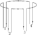
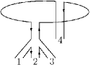
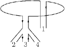
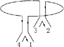
Figure 28: Color factors associated with the four gluon amplitude with planar color structure can be deformed to coincide with the momentum structure of the solution in terms of $\mathcal{D}_{2}$. Above we show the ordering (1234).

For the sum of these planar four gluon amplitudes, it is convenient to define, following [7], an effective $2\to 4$ vertex $V^{\text{R}}$, which sums the various decay-channels of the two reggeized gluons,

$$V^{\text{R}}({\bf l}_{1},{\bf l}_{2};{\bf k}_{1},{\bf k}_{2},{\bf k}_{3},{\bf k}_{4})=-{\bf l}_{1}^{2}{\bf l}_{2}^{2}\bigg{[} \delta^{(2)}({\bf l}_{1}-{\bf k}_{1}-{\bf k}_{2}-{\bf k}_{3})+\delta^{(2)}({\bf l}_{1}-{\bf k}_{1}-{\bf k}_{2}-{\bf k}_{4})$$

$$+\delta^{(2)}({\bf l}_{1}-{\bf k}_{1}-{\bf k}_{3}-{\bf k}_{4})+\delta^{(2)}({\bf l}_{1}-{\bf k}_{2}-{\bf k}_{3}-{\bf k}_{4})$$

$$- \delta^{(2)}({\bf l}_{1}-{\bf k}_{1}-{\bf k}_{2})-\delta^{(2)}({\bf l}_{1}-{\bf k}_{1}-{\bf k}_{3})-\delta^{(2)}({\bf l}_{1}-{\bf k}_{1}-{\bf k}_{4})\bigg{]},$$ (87)

such that

$$\sum_{(\text{ijkl})=\begin{subarray}{c}(1234),(2143),\\ (2134),(1243)\end{subarray}}\!\!\!\!\!\!\mathcal{D}_{4}^{(\text{ijkl})}(\omega|{\bf k}_{1},{\bf k}_{2},{\bf k}_{3},{\bf k}_{4})=\frac{\bar{\lambda}}{N_{c}}V^{(\text{R})}\otimes\mathcal{D}_{2}(\omega).$$ (88)

It is instructive to compare the results of this section with the finite $N_{c}$ results of [7]. For finite $N_{c}$ it was found that the four gluon amplitude $D_{4}$ can be written as a sum of two terms, the reggeizing term and the triple Pomeron vertex:

$$D_{4}=D_{4}^{R}+D_{4}^{I}$$ (89)

This decomposition was motivated by $t$-channel requirements: the reggeizing pieces contained in $D_{4}^{R}$ are antisymmetric under the exchange of the pair of gluons which forms the reggeized gluon, whereas the remainder $D_{4}^{I}$ (which contains the triple Pomeron vertex), is completely symmetric. In the present approach which is based upon the expansion in topologies, this decomposition into reggeizing and non-reggeizing pieces comes automatically, as a consequence of different classes of color structures. This suggests that the reggeization is deeply linked to the planar structure of scattering amplitudes.

6 The triple Pomeron vertex on the pair-of-pants

In this section we turn now to the partial wave amplitude associated with the non-planar class, $\mathcal{D}_{4}^{(\text{NP})}(\omega)$. As we have outlined at the end of Sec.4.6, we have to convolute, in Fig.25a - c, the branching vertices with $\mathcal{D}_{4}$, $\mathcal{D}_{3}$, and $\mathcal{D}_{2}$. Let us go through these convolutions in more detail.

We begin with those contributions where the branching vertex consists of a two-to-two transition (Fig.25a). They are to be combined with of one of the four planar amplitudes discussed before. Contributions involving $\mathcal{D}_{4}^{(1234)}(\omega)$ are

$$\parbox{56.9055pt}{ \includegraphics[width=56.9055pt]{trans12_2pop1234.ps}}+\parbox{56.9055pt}{\includegraphics[width=56.9055pt]{trans13_2pop1234.ps}}+\parbox{56.9055pt}{\includegraphics[width=56.9055pt]{trans24_2pop1234.ps}}+\parbox{56.9055pt}{ \includegraphics[width=56.9055pt]{trans34_2pop1234.ps}}\to\bar{g}^{2}N_{c}\sum_{\begin{subarray}{c}(12),(13),\\ (24),(34)\end{subarray}}K_{2\to 2}\otimes\mathcal{D}_{4}^{(1234)}(\omega),$$ (90)

where, on the rhs, the subscripts under the sum indicate which pairings of gluons should be included. A comment on the first and the last terms is in place. These interactions are inside the gluon pairs (12) or (34) and thus do not belong to the production of an $s$-channel gluon inside the $M^{2}$ discontinuity. Hence, these interactions are not part of the branching vertex. It is only for our convenience that we, nevertheless, include them into our definition of $\mathcal{D}_{4}^{(\text{NP})}(\omega)$ (later on, when defining the partial waves, we will have to subtract them again). In (90), the second and third term (the interactions (13) and (24)) carry an additional minus sign, due to the color structure (see Sec.4.3). Similarly one has

$$\parbox{56.9055pt}{ \includegraphics[width=56.9055pt]{leg2134_12.ps}}+\parbox{56.9055pt}{\includegraphics[width=56.9055pt]{pop23_2134.ps}}+\parbox{56.9055pt}{\includegraphics[width=56.9055pt]{pop14_2134.ps}}+\parbox{56.9055pt}{ \includegraphics[width=56.9055pt]{leg2134_34.ps}}\to\bar{g}^{2}N_{c}\sum_{\begin{subarray}{c}(12),(23),\\ (14),(34)\end{subarray}}K_{2\to 2}\otimes\mathcal{D}_{4}^{(2134)}(\omega),$$ (91)

while the contributions containing $\mathcal{D}_{4}^{(2143)}(\omega)$ and $\mathcal{D}_{4}^{(1243)}(\omega)$ are

$$\bar{g^{2}}N_{c}\sum_{\begin{subarray}{c}(12),(13),\\ (24),(34)\end{subarray}}K_{2\to 2}\otimes\mathcal{D}_{4}^{(2143)}(\omega)+\bar{g}^{2}N_{c}\sum_{\begin{subarray}{c}(12),(23),\\ (14),(34)\end{subarray}}K_{2\to 2}\otimes\mathcal{D}_{4}^{(1243)}(\omega).$$ (92)

In all three sums, the second and third terms carry minus signs, and the first and last terms are kept for convenience and will have to be removed later on.

For the two-to-three transition (Fig.25b) we have two contributions: terms that originate from $\mathcal{D}_{3}^{(123)}(\omega)$ are given by

$$\parbox{56.9055pt}{ \includegraphics[width=56.9055pt]{pop2_trans23.ps}}+\parbox{56.9055pt}{ \includegraphics[width=56.9055pt]{trans124_3pop1234.ps}}+\parbox{56.9055pt}{ \includegraphics[width=56.9055pt]{trans134_3pop1234.ps}}+\parbox{56.9055pt}{ \includegraphics[width=56.9055pt]{trans234_3pop1234.ps}}\to{\bar{g}}^{3}N_{c}\sum K_{2\to 3}\otimes\mathcal{D}_{3}^{(123)}(\omega),$$ (93)

where, on the rhs, the sum is over the four possible two-to-three transitions, allowed by the triple discontinuity. Again, in the second and the third terms a minus sign originating from the color factor has to be included. Contributions with $\mathcal{D}_{3}^{(321)}(\omega)$ are

$$\parbox{56.9055pt}{ \includegraphics[width=56.9055pt]{trans123_3pop1234.ps}}+\parbox{56.9055pt}{ \includegraphics[width=56.9055pt]{trans124_3popb.ps}}+\parbox{56.9055pt}{ \includegraphics[width=56.9055pt]{trans134_3popb.ps}}+\parbox{56.9055pt}{ \includegraphics[width=56.9055pt]{pop3_trans23.ps}}\to{\bar{g}}^{3}(-N_{c})\sum K_{2\to 3}\otimes\mathcal{D}_{3}^{(321)}(\omega),$$ (94)

where the sum is again over all four possible two-to-three transitions and for the second and third term a relative minus sign has to be included. Finally, from the two-to-four transition (Fig.25c) we have two contributions. They are given by

$$\parbox{56.9055pt}{\includegraphics[width=56.9055pt]{trans_4popx.ps}}+\parbox{56.9055pt}{\includegraphics[width=56.9055pt]{pop2_trans24.ps}}\to 2{\bar{g}^{4}}{N_{c}}K_{2\to 4}\otimes\mathcal{D}_{2}(\omega).$$ (95)

Combining these three groups and including the Reggeon-propagators we obtain for the amplitude $\mathcal{D}^{\text{NP}}_{4}$:

$$(\omega-\sum_{i}^{4}\beta({\bf{k}}_{i})\mathcal{D}^{\text{NP}}_{4}(\omega|{\bf k}_{1},{\bf k}_{2},{\bf k}_{3},{\bf k}_{4}) ={\bar{g}}^{3}N_{c}\sum K_{2\to 3}\otimes\mathcal{D}_{3}^{(123)}(\omega)+{\bar{g}}^{3}(-N_{c})\sum K_{2\to 3}\otimes\mathcal{D}_{3}^{(321)}(\omega)$$

$$+2{\bar{g}^{4}}{N_{c}}K_{2\to 4}\otimes\mathcal{D}_{2}(\omega)+\bar{g}^{2}N_{c}\bigg{[} \sum_{\begin{subarray}{c}(12),(13),\\ (24),(34)\end{subarray}}K_{2\to 2}\otimes\mathcal{D}_{4}^{(1234)}(\omega)+\sum_{\begin{subarray}{c}(12),(13),\\ (24),(34)\end{subarray}}K_{2\to 2}\otimes\mathcal{D}_{4}^{(2143)}(\omega)$$

$$+\sum_{\begin{subarray}{c}(12),(23),\\ (14),(34)\end{subarray}}K_{2\to 2}\otimes\mathcal{D}_{4}^{(2134)}(\omega)+\sum_{\begin{subarray}{c}(12),(23),\\ (14),(34)\end{subarray}}K_{2\to 2}\otimes\mathcal{D}_{4}^{(1243)}(\omega)\bigg{]}.$$ (96)

In the next step we make use of the fact that, according to the results of Sec.5.2 and Sec.5.4, all planar three and four gluon partial amplitudes on the rhs, $\mathcal{D}_{3}$ and $\mathcal{D}_{4}$, can be written as superpositions of two gluon amplitudes $\mathcal{D}_{2}(\omega)$. As a result, the right hand side of Eq.(6) depends only on $\mathcal{D}_{2}(\omega)$, convoluted with the sum of transition kernels:

$$(\omega-\sum_{i=1}^{4}\beta({\bf k}_{i}))\mathcal{D}_{4}^{\text{NP}}(\omega|{\bf k}_{1},{\bf k}_{2},{\bf k}_{3},{\bf k}_{4})= \frac{\bar{\lambda}^{2}}{N_{c}}V_{\text{TPV}}\otimes\mathcal{D}_{2}(\omega).$$ (97)

The right hand side of Eq.(97) defines the Triple-Pomeron-Vertex $V_{\text{TPV}}$ on the pairs-of-pants. It describes the coupling of the upper BFKL Pomeron, $\mathcal{D}_{2}(\omega)$, to the lower ones, $\mathcal{D}_{2}(\omega_{1})$ and $\mathcal{D}_{2}(\omega_{2})$.

The function $V_{\text{TPV}}$ coincides with the $V$ function found in [7]. In this paper, a finite $N_{c}$ calculation with $N_{c}=3$ has been carried out, and the following result for the $2\to 4$ gluon vertex has been obtained:

$$V_{2\to 4}^{a_{1}a_{2}a_{3}a_{4}}({\bf l}_{1},{\bf l}_{2}|{\bf k}_{1},{\bf k}_{2},{\bf k}_{3},{\bf k}_{4})) =\delta^{a_{1}a_{2}}\delta^{a_{3}a_{4}}V({\bf l}_{1},{\bf l}_{2}|{\bf k}_{1},{\bf k}_{2};{\bf k}_{3},{\bf k}_{4}))$$

$$+\,\delta^{a_{1}a_{3}}\delta^{a_{2}a_{4}} V({\bf l}_{1},{\bf l}_{2}|{\bf k}_{1},{\bf k}_{3};{\bf k}_{2},{\bf k}_{4}))+\delta^{a_{1}a_{4}}\delta^{a_{2}a_{3}}V({\bf l}_{1},{\bf l}_{2}|{\bf k}_{1},{\bf k}_{4};{\bf k}_{2},{\bf k}_{3}).$$ (98)

Here $a_{i}$, $i=1,\ldots 4$ denote color indices in the adjoint representation of the $t$-channel gluons. To compare with our result, we use the finite $N_{c}$ version of Eq.(6) in [17] which has been obtained for arbitrary $N_{c}$ and we find

$$\frac{\bar{\lambda}^{2}}{N_{c}}V_{\text{TPV}}({\bf l}_{1},{\bf l}_{2}|{\bf k}_{1},{\bf k}_{2};{\bf k}_{3},{\bf k}_{4}))=N_{c}V({\bf l}_{1},{\bf l}_{2}|{\bf k}_{1},{\bf k}_{2};{\bf k}_{3},{\bf k}_{4})).$$ (99)

It is easy to verify that this result is in complete agreement with the large large-$N_{c}$ limit of [7, 17]. Namely, if we project, in Eq.(6), on the color single state of the gluon-pairs (12)and (34) and then consider the limit of large $N_{c}$, only the first term on the right hand side of Eq.(6) contributes, and we indeed obtain agreement of the two results as required. In [8] it has been shown that the vertex $V$ is invariant under Möbius transformations. Furthermore, $V$ can be expressed in terms of another function $G({\bf k}_{1},{\bf k}_{2},{\bf k}_{3})$:

$$V({\bf k}_{1},{\bf k}_{2},{\bf k}_{3},{\bf k}_{4})= \bar{\lambda}\big{[}G(1,23,4)+G(2,13,4)+G(1,24,3)+G(2,14,3)-G(12,3,4)$$

$$-G(12,4,3)-G(1,2,34)-G(2,1,34)+G(12,-,34)\big{]},$$ (100)

where we suppressed the dependence on the momenta ${\bf l}_{1}$ and ${\bf l}_{2}$. This function $G$ has been first introduced for the forward case and $N_{c}=3$ in [7], whereas the above version was introduced in [10]. It has the nice property that it is not only infra-red finite but also by itself invariant under Möbius transformations [10].

7 The six-point amplitude on the pair-of-pants surface

With the results of the previous sections, we have almost all constituents that are needed to build the triple Regge limit of the six-point amplitude with the pair-of-pants topology. However before we add together the amplitudes of the foregoing sections, we need to take care of a peculiarity inside the planar piece of the upper amplitude. To leading order in $\lambda$, the two lower Pomerons couple directly to the upper quark-loop, as depicted in Fig.29 and the branching vertex is not given by a real gluon, but by the quark-loop itself. As long as we have, in addition to the $q\bar{q}$ pair, one (or more) $s$-channel gluons that contribute to the $M^{2}$ discontinuity, the mass of the $q\bar{q}$-system is integrated over, and this integration enters into the definition of the impact factors $\mathcal{D}_{4;0}^{(\text{ijkl})}$. Without such gluons, the mass of the $q\bar{q}$ pair coincides with the diffractive mass $M$ which is a fixed external parameter. In this case, the coupling of the $t$-channel four gluon system to the quark-loop is hence given by the triple discontinuity of the quark loop without the integration over the diffractive mass of the $q\bar{q}$-system, and defines an ’unintegrated’ four gluon impact factor, $\bar{\mathcal{D}}_{(4;0)}(M^{2})$. Its precise analytic form can be obtained from Eq.(2.8) of [7]. Correspondingly, its Mellin transform, which enters the partial wave $F(\omega,\omega_{1},\omega_{2})$ will be denoted by $\bar{\mathcal{D}}_{(4;0)}(\omega)$. When $\bar{\mathcal{D}}_{(4;0)}(M^{2})$ is integrated over the squared diffractive mass $M^{2}$, it coincides with sum over the impact factors $\mathcal{D}_{4;0}^{(\text{ijkl)}}$.

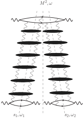
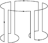
Figure 29: Diagrams where the two Pomerons couple directly to the upper quark-loop. They contain the lowest order diagram in Fig.11. The color factors can be reduced to the color factor to the right and therefore belong to the planar class.

After this remark we write the final result as the sum of two terms:

$$F(\omega,\omega_{1},\omega_{2})=F^{(\text{P})}(\omega,\omega_{1},\omega_{2})+F^{(\text{NP})}(\omega,\omega_{1},\omega_{2}),$$ (101)

where the first term sums the planar diagrams (including the ’unintegrated’ impact factors), the second term the non-planar ones. When doing the convolution of the three amplitudes, special care has to be taken of the counting of interactions inside the gluon pairs (12) and (34) just below the branching point where the upper cylinder splits into two cylinders (c.f. the discussion given in Sec.4.6). This issue has been addressed, for the ’$N_{c}$-finite’ case, in Sec.4 of [7] (see, in particular Eqs.(4.14) and Eq.(4.15)), and in the following we shall apply the same line of arguments. We identify, for the $M^{2}$ discontinuity, the lowest $s$-channel intermediate state which leads to the ’last’ interaction between the two gluon pairs (12) and (34): below this interaction, the upper cylinder has split into two separate cylinders. In particular, this last interaction cannot consist of a two-to-two kernel acting on the gluon pairs (12) or (34). Since, in Secs.5.3 and 6, we have defined the functions $\mathcal{D}_{4}^{(\text{ijkl})}$ and $\mathcal{D}_{4}^{(\text{NP})}$ in such a way that the last interaction includes these contributions, we first have to remove them. Furthermore, as explained above, the coupling of the $\mathcal{D}^{(12)}_{2}(\omega_{1})$ and $\mathcal{D}^{(34)}_{2}(\omega_{2})$ directly to the upper quark-loop is described by $\bar{\mathcal{D}}_{4;0}(\omega)$, and we write this term separately. We therefore arrive at the full partial wave in the following form:

$$F(\omega,\omega_{1},\omega_{2}) =4\mathcal{D}^{(12)}_{2}(\omega_{1})\otimes_{12}\mathcal{D}^{(34)}_{2}(\omega_{2})\otimes_{34}$$

$$\bigg{(}\bar{\mathcal{D}}_{(4;0)}(\omega)+\big{[}\omega-\sum_{i=1}^{4}\beta({\bf k}_{i})\big{]}\!\!\!\!\sum_{(\text{ijkl})=\begin{subarray}{c}(1234),(2143),\\ (2134),(1243)\end{subarray}}\!\!\!\!\mathcal{D}_{4}^{(\text{ijkl})}(\omega)+\frac{{\bar{\lambda}}^{2}}{N_{c}}V_{\text{TPV}}\otimes\mathcal{D}_{2}(\omega)$$

$$-2{\bar{\lambda}}(K^{(12)}_{2\to 2}+K^{(34)}_{2\to 2})\otimes\!\!\!\!\sum_{(\text{ijkl})=\begin{subarray}{c}(1234),(2143),\\ (2134),(1243)\end{subarray}}\!\!\!\!\mathcal{D}_{4}^{(\text{ijkl})}(\omega)\bigg{)}$$ (102)

In the first line, the indices of the convolution symbols indicate that $\mathcal{D}^{(12)}_{2}(\omega_{1})$ and $\mathcal{D}^{(34)}_{2}(\omega_{2})$ are to be contracted with the gluons (12) and (34), resp. The last line subtracts the two-to-two kernels acting on gluon pairs (12) and (34). Using the BFKL-equation

$$2\bar{\lambda}{K}_{2\to 2}^{(12)}\mathcal{D}^{(12)}_{2}(\omega_{1})=(\omega_{1}-\beta({\bf k}_{1})-\beta({\bf k}_{2}))\mathcal{D}^{(12)}_{2}(\omega_{1})-\mathcal{D}^{(12)}_{(2;0)}$$

(and a similar expression for the gluon pair (34)), and making further use of Eq.(88), we arrive at

$$F(\omega,\omega_{1},\omega_{2})=$$

$$\quad 4\bigg{\{}\mathcal{D}^{(12)}_{2}(\omega_{1})\otimes_{12}\!\mathcal{D}^{(34)}_{2}(\omega_{2})\otimes_{34}\!\bigg{(}\bar{\mathcal{D}}_{(4;0)}(\omega)+\big{[}\omega\!-\!\omega_{1}\!-\!\omega_{2}\big{]}V^{\text{R}}\!\otimes\!\mathcal{D}_{2}(\omega)+\frac{\bar{\lambda}^{2}}{N_{c}}V_{\text{TPV}}\!\otimes\!\mathcal{D}_{2}(\omega)\bigg{)}$$

$$\qquad+\mathcal{D}^{(12)}_{2}(\omega_{1})\otimes_{12}\mathcal{D}^{(34)}_{(2;0)}\otimes_{34}V^{\text{R}}\otimes\mathcal{D}_{2}(\omega)+\mathcal{D}^{(12)}_{(2;0)}\otimes_{12}\mathcal{D}^{(34)}_{2}(\omega_{2})\otimes_{34}V^{\text{R}}\otimes\mathcal{D}_{2}(\omega)\bigg{\}}.$$ (103)

The terms in the last line are either independent of $\omega_{2}$ or $\omega_{1}$ and the integrals over $\omega_{2}$ or $\omega_{1}$ vanish in Eq.(33). We therefore drop these terms and obtain for the two partial waves $F^{(\text{P})}(\omega,\omega_{1},\omega_{2})$ and $F^{(\text{NP})}(\omega,\omega_{1},\omega_{2})$ the following results:

$$F^{(\text{P})}(\omega,\omega_{1},\omega_{2}) =4\mathcal{D}^{(12)}_{2}(\omega_{1})\otimes_{12}\mathcal{D}^{(34)}_{2}(\omega_{2})\otimes_{34}\bigg{(}\bar{\mathcal{D}}_{(4;0)}(\omega)+\big{[}\omega-\omega_{1}-\omega_{2}\big{]}\frac{\bar{\lambda}}{N_{c}}V^{R}\otimes\mathcal{D}_{2}(\omega)\bigg{)}$$ (104)

and

$$F^{(\text{NP})}(\omega,\omega_{1},\omega_{2}) =4\mathcal{D}^{(12)}_{2}(\omega_{1})\otimes_{12}\mathcal{D}^{(34)}_{2}(\omega_{2})\otimes_{34}\frac{\bar{\lambda}^{2}}{N_{c}}V_{(\text{TPV})}\otimes\mathcal{D}_{2}(\omega).$$ (105)

Both terms are illustrated in Figs.30a and 30b.

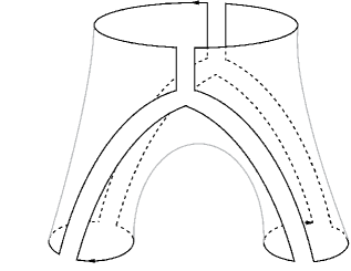
(a)

(b)

Figure 30: (a) Planar color graphs associated with the decay of two reggeized gluons and (b) non-planar color graphs which lead to the Triple-Pomeron-Vertex. In both cases a two gluon state decays into a four gluon state.

8 Conclusion

In the present analysis we have considered, in the large-$N_{c}$ limit, the triple Regge-limit of the scattering of three virtual photons. Our emphasis has been on the topology of color factors: we have summed, in the generalized leading-log approximation, only those diagrams which fit onto the pair-of-pants surfaces. These diagrams group themselves naturally into two classes (Fig.30). The first class consists of all diagrams which, by contracting closed color loops, coincide with one of the lowest order graphs (of order $g^{8}N_{c}^{3}$) illustrated in Fig.13. Making use of the bootstrap conditions, the sum of these graphs is shown to reduce to reggeized gluons with a simple splitting vertex. In addition, starting at the order $g^{8}N_{c}^{3}(g^{2}N_{c})$, a second class of diagrams appears which, by contracting closed color loops, cannot be drawn as one of the lowest order graphs shown in Fig.13. The sum of these graphs can be written as a convolution of three BFKL amplitudes, connected by the triple Pomeron vertex found in earlier papers. This triple Pomeron vertex has been shown to be invariant under Möbius transformation [8].

The analytic expression for the six-point amplitude derived in this paper coincides with the large-$N_{c}$ limit of the QCD result in [7]. However, the analysis of the present paper provides another interpretation of gluon reggeization and the appearance of the Möbius invariant triple Pomeron vertex: on the pair-of-pant surface, the reggeizing pieces are completely planar, whereas the the triple Pomeron vertex belongs to a distinct class of color diagrams which reflect the non-planar Mandelstam cross.

We believe that the topological approach pursued in this paper is well-suited for studying the Regge limit of N=4 Super Yang Mills Theory within the AdS/CFT correspondence. On the string side, amplitudes are naturally expanded in terms of topologies. In particular, the pair-of-pants topology studied in this paper is the same as that of the vertex which describes the coupling of three closed strings.

For a systematic study of the AdS/CFT correspondence it is convenient to make use of $R$-currents: they allow to formulate current correlators which are well-defined both on the gauge theory side and on the string side. As a first step of investigating, in the Regge limit, the duality between N=4 Super Yang Mills Theory and $AdS_{5}$ string theory, the 4-point function for such currents has been studied on the gauge theory side in [18]. This study confirms that the interaction between two $R$-currents in the Regge-limit is, indeed, mediated by a BFKL-Pomeron, and it contains the two gluon impact factors in N=4 SYM. On the string side, the scattering of two R-currents has been shown to involve, in lowest order, the one-graviton exchange [19]. In the present paper we have addressed, on the gauge theory side, the next term in the topological expansion. As a start, we have restricted ourselves to nonsupersymmetric QCD($N_{c}$). The generalization to the supersymmetric case where, inside the impact factors, fermions and scalar particles in the adjoint representation have to be considered, will be presented elsewhere [20]. On the string side, the analogous 6-point R-current correlator is expected to contain the triple graviton vertex. This project is currently being studied.

Acknowledgements

We thank L.N. Lipatov for helpful discussions. M.H. is grateful for financial support from the Graduiertenkolleg ”Zukünftige Entwicklungen in der Teilchenphysik” and from DESY.

References

- [1] G. ’t Hooft, Nucl. Phys. B 72 (1974) 461.
- [2] J. M. Maldacena, Adv. Theor. Math. Phys. 2 (1998) 231 [Int. J. Theor. Phys. 38 (1999) 1113] [arXiv:hep-th/9711200]; E. Witten, Adv. Theor. Math. Phys. 2 (1998) 253 [arXiv:hep-th/9802150]; S. S. Gubser, I. R. Klebanov and A. M. Polyakov, Phys. Lett. B 428 (1998) 105 [arXiv:hep-th/9802109].
- [3] L. N. Lipatov, Sov. J. Nucl. Phys. 23 (1976) 338 [Yad. Fiz. 23 (1976) 642]; V. S. Fadin, E. A. Kuraev and L. N. Lipatov, Phys. Lett. B 60 (1975) 50; Sov. Phys. JETP 44 (1976) 443 [Zh. Eksp. Teor. Fiz. 71 (1976) 840]; Sov. Phys. JETP 45 (1977) 199 [Zh. Eksp. Teor. Fiz. 72 (1977) 377]; I. I. Balitsky and L. N. Lipatov, Sov. J. Nucl. Phys. 28 (1978) 822 [Yad. Fiz. 28 (1978) 1597].
- [4] V. S. Fadin and L. N. Lipatov, Phys. Lett. B 429 (1998) 127 [arXiv:hep-ph/9802290], M. Ciafaloni and G. Camici, Phys. Lett. B 430 (1998) 349 [arXiv:hep-ph/9803389].
- [5] J. Bartels, Nucl. Phys. B 175 (1980) 365; J. Kwiecinski and M. Praszalowicz, Phys. Lett. B 94 (1980) 413.
- [6] L. N. Lipatov, JETP Lett. 59 (1994) 596 [Pisma Zh. Eksp. Teor. Fiz. 59 (1994) 571]; L. D. Faddeev and G. P. Korchemsky, Phys. Lett. B 342 (1995) 311 [arXiv:hep-th/9404173].
- [7] J. Bartels and M. Wusthoff, Z. Phys. C 66 (1995) 157.
- [8] J. Bartels, L. N. Lipatov and M. Wusthoff, Nucl. Phys. B 464 (1996) 298 [arXiv:hep-ph/9509303].
- [9] M. Braun, Z. Phys. C 71, 601 (1996) [arXiv:hep-ph/9502403], Eur. Phys. J. C 6, 321 (1999) [arXiv:hep-ph/9706373].
- [10] M. A. Braun and G. P. Vacca, Eur. Phys. J. C 6 (1999) 147 [arXiv:hep-ph/9711486].
- [11] S. R. Coleman, “1/N”, in Aspects of Symmetry, Cambridge University Press, Cambridge, 1985, A. V. Manohar, “Large N QCD,” arXiv:hep-ph/9802419.
- [12] H. H. Matevosyan and A. W. Thomas, J. Phys. G 35 (2008) 115006.
- [13] G. ’t Hooft, Nucl. Phys. B 75 (1974) 461.
- [14] M. Braun, Z. Phys. C 73 (1997) 517.
- [15] V. Del Duca, Phys. Rev. D 48 (1993) 5133 [arXiv:hep-ph/9304259], Phys. Rev. D 52 (1995) 1527 [arXiv:hep-ph/9503340].
- [16] L. N. Lipatov, Sov. Phys. JETP 63 (1986) 904 [Zh. Eksp. Teor. Fiz. 90 (1986) 1536].
- [17] J. Bartels and C. Ewerz, JHEP 9909 (1999) 026 [arXiv:hep-ph/9908454].
- [18] J. Bartels, A.-M. Mischler and M. Salvadore, Phys. Rev. D 78 (2008) 016004 [arXiv:0803.1423 [hep-ph]].
- [19] J. Bartels, J. Kotanski, A.-M. Mischler and V. Schomerus, to be published
- [20] J. Bartels, C. Ewerz, M. Hentschinski and A.-M. Mischler, to be published