Shuttling heat across 1D homogenous nonlinear lattices with a Brownian heat motor

Abstract

We investigate directed thermal heat flux across 1D homogenous nonlinear lattices when no net thermal bias is present on average. A nonlinear lattice of Fermi-Pasta-Ulam-type or Lennard-Jones-type system is connected at both ends to thermal baths which are held at the same temperature on temporal average. We study two different modulations of the heat bath temperatures, namely: (i) a symmetric, harmonic ac-driving of temperature of one heat bath only and (ii) a harmonic mixing drive of temperature acting on both heat baths. While for case (i) an adiabatic result for the net heat transport can be derived in terms of the temperature dependent heat conductivity of the nonlinear lattice a similar such transport approach fails for the harmonic mixing case (ii). Then, for case (ii), not even the sign of the resulting Brownian motion induced heat flux can be predicted a priori. A non-vanishing heat flux (including a non-adiabatic reversal of flux) is detected which is the result of an induced dynamical symmetry breaking mechanism in conjunction with the nonlinearity of the lattice dynamics. Computer simulations demonstrate that the heat flux is robust against an increase of lattice sizes. The observed ratchet effect for such directed heat currents is quite sizable for our studied class of homogenous nonlinear lattice structures, thereby making this setup accessible for experimental implementation and verification.

I Introduction

In recent years, we have experienced a wealth of theoretical and experimental activities in the field of phononics, the science and engineering of phonons WangLi08 . Traditionally being regarded as a nuisance, phonons are found to be able to carry and process information as well as electrons do. The control and manipulation of phonons manifest itself in the form of theoretically designed thermal device models such as thermal diodes rectifier ; diode ; quantumdiode ; Hu06 ; peyrard ; yang , thermal transistors transistor , thermal logic gates WangLi07 and thermal memories wangli08 . The theoretical research has been accompanied by pioneering experimental efforts. In particular, the first realization of solid-state thermal diode has been put forward with help of asymmetric nanotubes experimentaldiode . Owing to the transport of phonons, the heat flow can be controlled the same way as electric currents.

Dwelling on ideas from the field of Brownian motors BM1 ; BM2 ; BM3 ; BM4 ; BM5 , – originally devised for Brownian particle transport, – a thermal ratchet based on a nonlinear lattice setup has been proposed in Ref. LHL . In absence of any stationary non-equilibrium bias, a non-vanishing net heat flow can be induced by non-biased, temporally alternating bath temperatures combined with a non-homogenous coupled nonlinear lattice structure. In the similar spirit of pumping heat on the molecular scale vandenbroeckPRL2006 ; segal2003 ; segalPRE2006 ; marathePRE2007 ; vandenbroeckPRL2008 , the heat flow can be directed against an external thermal bias.

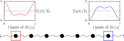
Figure 1: (Color-online) Schematic setup of a 1D homogenous nonlinear lattice, being coupled to two heat baths with periodically varying temperatures at $T_{L}(t)$ and $T_{R}(t)$.

With this work we propose a superior, easy to implement Brownian heat motor that can induce finite net heat flow for a homogenous, intrinsically symmetric lattice structure as depicted in Fig. 1. In doing so, the lattice system is brought into contact with two heat baths which both may be subjected to time-periodic temperatures, see Fig. 1. To obtain a finite directed heat current then requires a symmetry breaking. In this work we shall investigate two mechanisms of symmetry breaking by use of a temporal modulation of temperatures of heat baths.

Section II introduces our model for directing heat current through 1D lattice chains with temperature modulations applied to connecting heat baths. Section III presents analytical adiabatic theory and extensive numerical results for the case that temperature is time-modulated in one bath only, i.e. our case (i). In this case, an intrinsic nonlinear temperature dependence of the heat conductivity is sufficient to induce a shuttling of heat. Our main results are presented with Section IV: A more intriguing mechanism comes into play when applying an unbiased modulation of temperatures in both heat baths. Put differently, in order to eliminate the possibility of solely creating a non-vanishing net heat flux from the the temperature-dependent thermal conductivity $\kappa(T)$ we invoke a nonlinear harmonic mixing drive of temperature in both heat baths; i.e. our case (ii). The results are discussed and summarized in the Conclusions.

II Shuttling heat despite vanishing average temperature bias

Explicitly, we study numerically a 1D homogenous nonlinear lattice consisting of $N$ atoms of identical mass $m$. This setup is depicted in Fig. 1, with the following nonlinear lattice Hamiltonian:

$$H=\sum^{N}_{i=1}\frac{p^{2}_{i}}{2m}+\sum^{N}_{i=0}V(x_{i+1},x_{i})$$ (1)

where $x_{i}$ is the coordinate for $i$-th atom, and the distance between two neighboring atoms at equilibrium gives the lattice constant $a$. The interaction between nearest neighbors is described by $V(x_{i+1},x_{i})$. Here, fixed boundary conditions $x_{0}=0$ and $x_{N+1}=(N+1)a$ have been employed. The first and last atom are put into contact with two Langevin heat baths, generally possessing time-dependent temperatures $T_{L}(t)$ and $T_{R}(t)$, respectively. Moreover, Gaussian thermal white noises obeying the fluctuation-dissipation relation are used; i.e.,

$$\langle\xi_{1(N)}(t)\rangle = 0$$

$$\mathrm{and}\hskip 20.00003pt\langle\xi_{1(N)}(t)\xi_{1(N)}(0)\rangle = 2k_{B}\eta T_{L(R)}\delta(t)\;.$$ (2)

Here, $k_{B}$ denotes the Boltzmann constant and $\eta$ is the coupling strength between the system and the heat bath.

The time-varying heat bath temperature $T_{L}(t)$ and $T_{R}(t)$ are chosen as periodic functions $T_{L(R)}(t)=T_{L(R)}(t+2\pi/\omega)$ where $T_{0}=\overline{T_{L}(t)}=\overline{T_{R}(t)}$ is the temporally averaged, constant environmental reference temperature. Clearly, the coherent changes of these bath temperatures occur on a time-scale that is much smaller than the (white) thermal fluctuations itself. Importantly in present context, this so driven system dynamics exhibits a vanishing average thermal bias; i.e.,

$$\overline{\Delta T(t)}\equiv\overline{T_{L}(t)-T_{R}(t)}=0\;.$$ (3)

The time-dependent, asymptotic heat flux $J_{i}(t)$ is assuming the periodicity of the external driving period $2\pi/\omega$ after the transient behavior has died out LHL . This feature is confirmed in our numerical simulations (not shown here). At those asymptotic long times, the resulting heat flux equals the thermal Brownian noise average HuLiZhao :

$$J_{i}(t)=\left<\dot{x}_{i}\partial{V(x_{i+1},x_{i})}/\partial{x_{i}}\right>\;.$$ (4)

The stationary heat flux $\bar{J}$ then follows as the cycle average over a full temporal period; i.e.,

$$\overline{J(t)}:=\bar{J} = \frac{\omega}{2\pi}\int_{0}^{2\pi/\omega}\left<\dot{x}_{i}\partial{V(x_{i+1},x_{i})}/\partial{x_{i}}\right>dt$$ (5)

$$= \frac{\omega}{2\pi}\int_{0}^{2\pi/\omega}J_{i}(t)dt\;,$$

which after averaging becomes independent of atom position $i$. With ergodicity being obeyed, this double-average equals as well the long time average

$$\bar{J} =\overline{\dot{x}_{i}\partial{V(x_{i+1},x_{i})}/\partial{x_{i}}}$$

$$=\lim_{t\rightarrow\infty}\frac{1}{t}\int_{0}^{t}\dot{x}_{i}(t)\partial{V(x_{i+1},x_{i})}/\partial{x_{i}}|_{t}dt\;.$$ (6)

Here, the temporal average is over corresponding stochastic trajectories entering the relation in Eq. (5). We emphasize that the resulting ratcheting heat flux involves an average over the Brownian thermal noise forces. Put differently, the flux is not determined by a deterministic molecular dynamics but rather by the driven nonlinear Langevin dynamics following from the nonlinear lattice dynamics in Eq. (1) and being complemented with Langevin forces obeying the fluctuation-dissipation relation in Eq. (II). This in turn defines our Brownian heat motor dynamics.

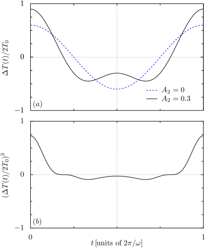
Figure 2: (Color-online) Modulating the bath temperature. The temperature bias $\Delta T(t)\equiv T_{L}(t)-T_{R}(t)$ is depicted over a full driving period without and with a second harmonic driving term, panel(a). The strength $A_{1}=0.6$ is chosen for both cases. The third moment of the harmonic mixing signal $(\Delta T(t)/2T_{0})^{3}$ is shown with panel (b). Note that in distinct contrast to the unbiased first moment the cycle average of this odd third moment is now nonvanishing.

III Rocking temperature of one heat bath only

We start out by considering that only the temperature of the left heat bath is subjected to a time-varying modulation, i.e. our case (i) is defined by setting

$$T_{L}(t):=T_{L} = T_{0}[1+A_{1}\cos{(\omega t)}]$$

$$T_{R}(t):=T_{R} = T_{0}\;.$$ (7)

The symmetric temperature difference $\Delta T(t)/2T_{0}$ over one period is depicted in Fig. 2(a) as the dashed line.

The Fermi-Pasta-Ulam $\beta$ (FPU-$\beta$) lattice is used for illustration, where the potential term $V(x_{i+1},x_{i})$ assumes the following form:

$$V(x_{i+1},x_{i})=\frac{k}{2}(x_{i+1}-x_{i}-a)^{2}+\frac{\beta}{4}(x_{i+1}-x_{i}-a)^{4}$$ (8)

We introduce the dimensionless parameters by measuring positions in units of $a$, momenta in units of $[a(mk)^{1/2}]$, temperature in units of $[ka^{2}/k_{B}]$, spring constants in units of $k$, frequencies in units of $[(k/m)^{1/2}]$ and energies in units of $[ka^{2}]$. The equations of motion are integrated by the symplectic velocity Verlet algorithm with a small time step $h=0.005$. The system is simulated at least for a total time $t_{tot}=2\cdot 10^{8}$. The chosen optimal coupling strength of the heat bath is fixed at $\eta=0.5$. In the following simulations, we will take the dimensionless parameters $k=1,\beta=1$.

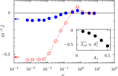
Figure 3: (Color-online) One-sided temperature modulation. The cycle averaged ratcheting heat flux $\bar{J}$ in a nonlinear FPU-$\beta$ lattice is depicted as the function of the driving frequency $\omega$. The hollow (red) circles are the results for harmonic drive $A_{1}\cos(\omega t)$ with $A_{1}=0.5$; the filled (blue) circles are the results for a weaker driving strength at $A_{1}=0.2$. The simulations are performed on a FPU-$\beta$ lattice with $N=50$ atoms and with a reference temperature set at $T_{0}=0.5$. The arrows pointing towards the left mark the adiabatic linear transport result from Eq. (9), see text. Inset is the figure for $\overline{J_{ad}}$ as the function of $A_{1}$ and $\overline{J_{ad}}$ has the basic units $[10^{-3}]$.

The net heat flux $\bar{J}$ as a function of driving frequency $\omega$ is depicted in Fig. 3. In the adiabatic limit $\omega\rightarrow 0$, a negative ratchet heat flux is obtained. In the high frequency limit $\omega\rightarrow\infty$, the left- and right-end atoms will experience a time-averaged constant temperature. This corresponds to effective thermal equilibrium, yielding $\bar{J}\rightarrow 0$ when $\omega\rightarrow\infty$. In the non-adiabatic limit we even observe a reversal of heat flux, although not very pronounced.

When the temperature is modulated slowly enough, the periodic influence of dynamical thermal bias can be viewed as the average, integrated quasi-stationary flux induced by the momentarily static thermal bias, i.e. $J_{i}(t)=J_{i}(\Delta T(t)/N)$. In the linear transport regime, this flux can be expressed as a linear transport Law, reading $J_{i}(t)=\kappa\left((T_{L}(t)+T_{R}))/2\right)\Delta T(t)/N$. Here the temperature value of the size (N)-dependent thermal conductivity of the FPU lattice must be determined numerically at the midpoint of the, in this adiabatic case, linearly varying temperature profile EPL_lnb . Thus, the adiabatic net heat flux assumes in leading order the result

$$\overline{J_{ad}} = \frac{\omega}{2\pi}\int^{2\pi/\omega}_{0}dt\,\kappa\left(\frac{T_{L}(t)+T_{R}}{2}\right)\frac{T_{L}(t)-T_{R}}{N}$$ (9)

$$= \frac{\omega}{2\pi}\int^{2\pi/\omega}_{0}dt\,\kappa\left(T_{0}+\frac{A_{1}T_{0}\cos{(\omega t)}}{2}\right)\frac{A_{1}T_{0}\cos{(\omega t)}}{N}$$

$$= \frac{\omega}{2\pi}\int^{\pi/\omega}_{0}dt\,\left[\kappa\left(T_{0}+\frac{A_{1}T_{0}\sin{(\omega t)}}{2}\right)\right.$$

$$\,\,\,\,\,\,\,\,\,\,\,\,\,\,\,\,\,\,\,\,\,\,\,\,\,\,\,\,\,\,\left.-\kappa\left(T_{0}-\frac{A_{1}T_{0}\sin{(\omega t)}}{2}\right)\right]\frac{A_{1}T_{0}\sin{(\omega t)}}{N}$$

$$< 0\;.$$

The predicted sign on last line in the above expression originates from the following reasoning: For the considered FPU-$\beta$ lattice the thermal conductivity possesses a temperature-dependent behavior $\kappa(T)\propto 1/T$ in the regime of dimensionless temperature $T(t)<1$ EPL_lnb . With the reference temperature $T_{0}=0.5$, $\kappa\left(T_{0}+\frac{A_{1}\sin{(\omega t)}}{2}T_{0}\right)$ is alwaysf less than $\kappa\left(T_{0}-\frac{A_{1}\sin{(\omega t)}}{2}T_{0}\right)$ in the time window of $[0,\pi/\omega]$. Therefore, a negative ratchet heat flux will result from the temperature modulation of only one heat bath as in Eq. (III). This prediction is corroborated with our numerical calculations in Fig. 3 for low driving frequencies $\omega$. Furthermore, the adiabatic value of $\overline{J_{ad}}$ can be approximately calculated from the quadrature in Eq. (9). This calculated adiabatic value is marked with the arrow pointing towards the left axis in Fig. 3. For small rocking strength, $A_{1}\ll 1$, this adiabatic prediction remarkably well agrees with the full nonlinear, asymptotic value, see in Fig. 3. For larger driving strengths $A_{1}$ the numerically precise full adiabatic result exhibits notable deviations from this linear transport Law estimate.

Taking into account the size dependent property of heat conductivity $\kappa(T,N)$, we can express $\overline{J_{ad}}$ further by taking a Taylor expansion for $\kappa\left(T_{0}+\frac{A_{1}\sin{(\omega t)}}{2}T_{0},N\right)$ and $\kappa\left(T_{0}+\frac{A_{1}\sin{(\omega t)}}{2}T_{0},N\right)$ at reference temperature $T_{0}$:

$$\overline{J_{ad}} = \frac{\omega}{2\pi}\int^{\pi/\omega}_{0}dt\,\left[\left.\frac{\partial{\kappa(T,N)}}{\partial{T}}\right|_{T_{0}}A_{1}T_{0}\sin{(\omega t)}+O(A_{1}^{3})\right]$$ (10)

$$\,\,\,\,\,\,\,\,\,\,\times A_{1}T_{0}\sin{(\omega t)}/N$$

$$\approx \frac{1}{4}A_{1}^{2}T_{0}^{2}\left.\frac{\partial\kappa(T,N)}{\partial{T}}\right|_{T_{0}}/N$$

$$\propto A_{1}^{2}N^{\alpha-1}$$

where in the last line we have used the fact that $\left.\frac{\partial\kappa(T,N)}{\partial{T}}\right|_{T_{0}}$ assumes the same size-dependence as $\kappa(T,N)$, i.e. $\kappa(T,N)\propto N^{\alpha}$ with $\alpha<1$ Lepri_pr . The non-zero adiabatic ratchet heat flux is a finite size effect since it vanishes in the limit $N\rightarrow\infty$ proportional to $N^{\alpha-1}$.

We numerically determined the adiabatic net heat flux by averaging heat flux from four lowest frequencies for each amplitude $A_{1}$. The amplitude effect $\overline{J_{ad}}\propto A_{1}^{2}$ is verified by our numerical calculations as can be seen in the inset of Fig. 3.

IV Rocking temperature in both heat baths

We next consider case (ii) with unbiased temperature modulations applied to both heat baths. The time-varying heat bath temperature $T_{L}(t)$ and $T_{R}(t)$ are chosen as:

$$T_{L}(t):=T_{L}=T_{0}[1+A_{1}\cos{(\omega t)}+A_{2}\cos{(2\omega t+\varphi)}]$$

$$T_{R}(t):=T_{R}=T_{0}[1-A_{1}\cos{(\omega t)}-A_{2}\cos{(2\omega t+\varphi)}]$$ (11)

where $T_{0}=\overline{T_{L}(t)}=\overline{T_{R}(t)}$. The overall averaged net temperature difference, $\overline{\Delta T(t)}\equiv\overline{T_{L}(t)-T_{R}(t)}=0$, is again unbiased as before. The driving amplitude $A_{1}$ and $A_{2}$ are taken as positive values and the relation $A_{1}+A_{2}\leq 1$ must be fulfilled to avoid negative temperatures. Note, however, that in distinct contrast to the situation with case (i) the time-dependent average temperature; i.e.,

$$T_{av}(t)\equiv[T_{L}(t)+T_{R}(t)]/2=T_{0}$$ (12)

is now time-independent. This feature excludes us from estimating the adiabatic heat flux within a linear transport Law of heat as exercised under case (i). Put differently, the temperature dependent, nonlinear thermal conductivity $\kappa(T)$ alone is not sufficient to set up an adiabatic heat flow, see below. A resulting finite heat flux is thus beyond the mere role of a nonlinear lattice and instead is the outcome of the nonlinear interplay of harmonic mixing of the two frequencies in the nonlinear lattice dynamics to yield a zero-frequency response for the time-averaged nonlinear heat flow as defined by Eqs. (5,6).

In more detail: The second harmonic driving $A_{2}\cos(2\omega t+\varphi)$ causes nonlinear frequency mixing. The temperature signal $\Delta T(t)$ notably is unbiased with zero average. It causes, however, a dynamical symmetry breaking EPL_luczka ; EPL_hanggi ; thus giving rise to directed transport EPL_luczka ; EPL_hanggi ; goychuk ; flach ; denisov . The time evolution of the harmonic mixing signal is depicted in Fig. 2(a) for a phase shift of $\varphi=0$ with the solid line. The second harmonic drive may typically contain a non-zero phase shift $\varphi$. In accordance with previous studies in single particle Brownian motors goychuk ; denisov the resulting current is expected to become maximal for $\varphi=0$. In the following we therefore stick in our numerical studies, if not stated otherwise, to a fixed vanishing phase-shift $\varphi=0$. Note that this drive with $\varphi=0$ is symmetric under time-reversal $t\longrightarrow-t$; nevertheless, time reversal is broken by the frictional Langevin dynamics acting upon the end atoms, see above.

The fact that a finite heat flux results when driven by harmonic mixing can be reasoned physically by noting that in contrast to the case with $A_{2}=0$: When $A_{2}\neq 0$, despite the vanishing temporal cycle average $\overline{\Delta T(t)}=0$, one deals with temporal temperature differences $\Delta T(t)$ that are no longer symmetric around $\Delta T(t)=0$, cf. 2(a). With this harmonic mixing modulation, all odd-numbered moments $(\overline{\Delta T(t))^{(2n+1)}}\neq 0$ , $n\geq 1$ are non-vanishing after the temporal cycle average. With heat flow in nonlinear systems typically being a function of the temperature bias beyond linear response regime, we thus nevertheless expect a net finite heat flux. This feature follows by observing that a leading nonlinear response due to the non-vanishing temporal cycle average of the third moment $\overline{(\Delta T(t)/2T_{0})^{3}}=(3/4)A_{1}^{2}A_{2}\cos{\varphi}$, see in Fig. 2(b), is non-vanishing. In clear contrast to a single particle case, see in Ref. goychuk ; BM5FN , the amplitude $A_{2}$ in our case (ii) assumes within $T_{L(R)}$ both signs. Therefore, one principally cannot even predict a priori the sign of the resulting heat current. This very fact is the benchmark of a truly Brownian heat motor where the external temperature modulation is only weakly coupled to the Brownian motion induced heat flow BM1 ; BM2 ; BM3 ; BM4 ; BM5 .

IV.1 Shuttling heat across a Fermi-Pasta-Ulam $\beta$ lattice

We start the study of case (ii) by considering the FPU-$\beta$ lattice of Eq. (8) by using the same parameters as before. The net heat flux $\bar{J}$ as a function of driving frequency $\omega$ is depicted in Fig. 4. For $A_{2}=0$, there indeed emerges no finite heat flux; this corroborates with theory because of the absence of dynamical symmetry breaking between positive and negative temperature differences $\Delta T(t)$, see Fig. 2. The non-zero second harmonic driving term with $A_{2}\neq 0$ globally causes with $\Delta T(t)\neq 0$ a dynamical symmetry breaking. At low, adiabatic driving frequencies $\omega\rightarrow 0$, we obtain a finite heat flux $\bar{J}\neq 0$ which is solely induced by dynamical symmetry breaking caused by harmonic mixing. Again, the heat flux $\bar{J}$ vanishes in the high frequency limit as expected.

Adiabatic estimate

An adiabatic analysis within a linear transport mechanism is no longer possible here: By noting that the average temperature $[T_{L}(t)+T_{R}(t)]/2=T_{0}$ is time-independent, the previous adiabatic estimate now reduces to:

$$\overline{J_{av}} = \frac{\omega}{2\pi}\int^{2\pi/\omega}_{0}dt\,\kappa\left(\frac{T_{L}(t)+T_{R}(t)}{2}\right)\frac{T_{L}(t)-T_{R}(t)}{N}$$ (13)

$$= \frac{\omega}{2\pi}\int^{2\pi/\omega}_{0}dt\,\kappa\left(T_{0}\right)\frac{\Delta T(t)}{N}$$

$$= 0\,;$$

i.e., it predicts a vanishing rachet heat flux. As mentioned above, the observed finite heat flux is due to a nonlinear interplay between the driving frequencies for which we are even not able to predict a priori the sign.

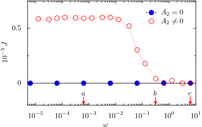
Figure 4: (Color-online) Ratcheting heat flux in the FPU-$\beta$-lattice. Cycle averaged heat flux $\bar{J}$ as the function of the driving frequency $\omega$. The solid circles are the results for symmetric harmonic driving with $A_{2}=0$. The hollow circles are the results for harmonic mixing with $A_{2}=0.3$ and a relative phase shift $\varphi=0$. The harmonic driving parameter is set for both cases at $A_{1}=0.6$. The simulations are performed on a FPU-$\beta$ lattice with $N=50$ atoms and with a reference temperature $T_{0}=0.5$. The three arrows indicate the distinct driving frequencies used in Fig. 5.

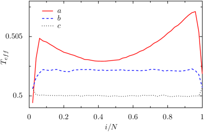
Figure 5: (Color-online) Effective temperature profiles of three selected frequencies for $A_{2}=0.3$ in Fig. 4 with $T_{0}=0.5$.

Local temperature profile

To gain further insight into this intriguing regime of finite ratchet heat flux, we investigate the local temperature variations across the chain at three distinct different driving frequencies $\omega$. The local (kinetic) temperature is defined via the equipartition theorem as the time average of kinetic energy $T_{eff}(i)=\overline{\dot{q}^{2}_{i}}$, as in Ref. LHL . The effective temperature profiles of three numerical runs, denoted as ($a,b,c$) in Fig. 4, are depicted in Fig. 5 versus the relative site position $i/N$. In clear contrast to the non-driven case with no temperature modulation, a distinct temperature profile emerges for the driven case. This averaged effective temperature $T_{eff}(i)$ lies typically above the time-independent average temperature $T_{av}=T_{0}$ with regimes of both, positive- and negative-valued local gradient. Even for the case of slow, adiabatic driving, i.e., case (a) in Fig. 5, we cannot now even detect a clear-cut mechanism to yield the now positive sign for the shuttled heat flux. This corroborates with our reasoning that no simple adiabatic estimate can be devised in this situation.

We also note that with identical signs for $A_{1},A_{2}$ of $T_{L(R)}(t)$ in Eq. (IV), implying that $\Delta T(t)=0$ identically, no ratchet heat flux can be detected (not shown).

IV.2 Shuttling heat across a Fermi-Pasta-Ulam $\alpha\beta$ lattice

We next consider the Fermi-Pasta-Ulam $\alpha\beta$ (FPU-$\alpha\beta$) lattice, where the potential term $V(x_{i+1},x_{i})$ assumes the following form:

$$V(x_{i+1},x_{i})=\frac{k}{2}(x_{i+1}-x_{i}-a)^{2}$$

$$\,\,\,\,+\frac{\alpha}{3}(x_{i+1}-x_{i}-a)^{3}+\frac{\beta}{4}(x_{i+1}-x_{i}-a)^{4}$$ (14)

In the simulations, we will employ the dimensionless parameters $k=1,\alpha=1,\beta=1/4$.

The net heat flux $\bar{J}$ for this system is depicted in Fig. 6. We again cannot detect any finite heat flux for $A_{2}=0$. For $A_{2}=0.3$, we now detect a negative ratchet heat flux in the low frequency, adiabatic limit. This ratchet heat flux vanishes as expected in the high frequency limit. Surprisingly however, the heat flux does not approach zero monotonically as in the case with the FPU-$\beta$ lattice. At some intermediate frequency range, the direction of the net heat flux reverses sign! We detect two distinct peaks for the heat flux of opposite directions that occur within a narrow frequency window.

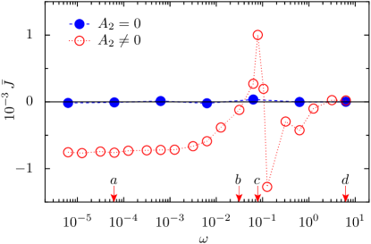
Figure 6: (Color-online) Ratcheting heat flux in a FPU-$\alpha\beta$ lattice. Cycle averaged heat flux $\bar{J}$ as the function of the driving frequency $\omega$. The solid circles are the results for symmetric harmonic driving with $A_{2}=0$. The hollow circles are the results for harmonic mixing with $A_{2}=0.3$ and a relative phase shift $\varphi=0$. The harmonic driving parameter is set for both cases at $A_{1}=0.6$. The simulations are performed on a FPU-$\alpha\beta$ lattice with $N=50$ atoms and with a reference temperature $T_{0}=1$, see text. The arrows indicate the driving frequencies used in Fig. 7.

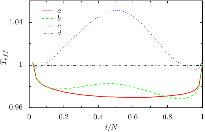
Figure 7: (Color-online) Effective temperature profiles for the four selected frequencies with $A_{2}=0.3$ depicted in Fig. 6. Here the average bath temperature is held at $T_{0}=1$.

We as well depict a plot for the local temperature variations across the chain at different driving frequencies $\omega$. The effective temperature profiles of four numerical runs, denoted as ($a,b,c,d$) in Fig. 6, are shown in Fig. 7 versus the relative site positions $i/N$. For frequencies near the flux-reversal point, the inner structure of effective temperature becomes very complicated and we could not detect a clear-cut connection between local temperature and the direction of ratcheting heat flux.

When the lattice size $N$ is increased, the thermal bias $\Delta T(t)/N$ is reduced. One therefore would expect a smaller heat flux $\bar{J}$. In Fig. 8, we plot $\bar{J}$ versus $\omega$ for three different lattice sizes $N=50,100,200$. Contrary to common intuition, however, the finite heat flux $\bar{J}$ in the adiabatic limit $\omega\rightarrow 0$ is practically independent of system size. This feature again corroborates with the fact that in this regime no obvious adiabatic estimate is deducible.

This result of a size-insensitivity will prove advantageous for the experimenters attempting to measure such directed ratchet heat flux, e.g. by use of a nanotube coupled in between two heat contacts.

The peaks of opposite directions are also found for larger system sizes. The positions of these peaks become red-shifted for larger system size $N$. This effect is related to the thermal response time as we have detailed before with Ref. LHL . The characteristic frequency can be estimated as $\omega_{c}\approx 8\pi\kappa(N)/cN^{2}$. The specific heat can be approximated as $c\approx 1$. The FPU lattice is well known to exhibit anomalous heat conduction with size-dependent thermal conductivities $\kappa(N)$ kabu ; lepri ; pere . The thermal conductivity $\kappa(N)$ at temperature $T=1$ has the following numerical values, $\kappa(50)=19.1,\kappa(100)=25.1$ and $\kappa(200)=32.9$. Thus, the characteristic frequencies can be estimated as $\omega_{c}\approx 0.19$ for $N=50$, $\omega_{c}\approx 0.063$ for $N=100$ and $\omega_{c}\approx 0.021$ for $N=200$. These values are marked as arrows pointing to $x$-axis in Fig. 8; these values impressively corroborate with numerical simulation results.

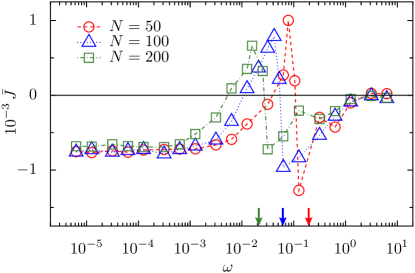
Figure 8: (Color-online) Size dependence of directed heat flux. Ratchet heat flux $\bar{J}$ vs. the driving frequency $\omega$ for different FPU-$\alpha\beta$ lattice sizes $N=50$ (circle), $N=100$ (triangle) and $N=200$ (square). The driving amplitudes are set at $A_{1}=0.6$, $A_{2}=0.3$ and $\varphi=0$. The estimate of the frequency scale set by the thermal response time which scales with the anomalous FPU-heat conductivity $\kappa(N)$.

IV.3 Directing heat across a Lennard-Jones lattice

We finally consider the physically realistic case of a Lennard-Jones (LJ) lattice. The interaction $V(x_{i+1},x_{i})$ for a LJ lattice interaction takes the form

$$V(x_{i+1},x_{i})=\epsilon\left[\left(\frac{a}{x_{i+1}-x_{i}}\right)^{12}-2\left(\frac{a}{x_{i+1}-x_{i}}\right)^{6}\right]\;,$$ (15)

where $a$ is the lattice constant and $\epsilon$ is the depth of the potential well. New dimensionless parameters can be introduced by measuring positions in units of $a$, momenta in units of $[(m\epsilon)^{1/2}]$, temperature in units of $[\epsilon/k_{B}]$, spring constants in units of $[\epsilon/a^{2}]$, frequencies in units of $[(\epsilon/ma^{2})^{1/2}]$ and energies in units of $\epsilon$. A particular material is described by the pair of parameters $a$ and $\epsilon$.

The resulting ratchet heat flux $\bar{J}$ for LJ-lattice is depicted in Fig. 9. Just as is the case in FPU lattice, we cannot detect finite flux $\bar{J}$ for pure harmonic driving with $A_{2}=0$. In the adiabatic limit $\omega\rightarrow 0$, a virtually size-independent finite heat flux $\bar{J}$ results when $A_{2}\neq 0$; i.e. the emerging ratchet heat flux is rather robust. In our simulations we used a dimensionless reference temperature $T_{0}=3$. To give a example, for Argon atoms with parameters $(a=3.4[\mathring{A}],\epsilon=119.8k_{B}[K])$, this dimensionless temperature $T_{0}$ corresponds to a physical temperature $T=T_{0}\epsilon/k_{B}=359.4[K]$.

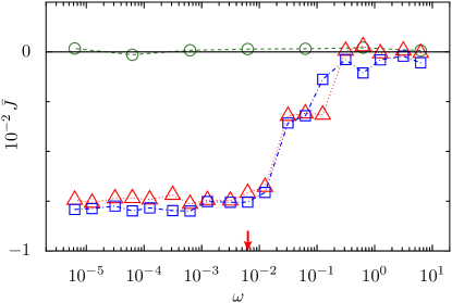
Figure 9: (Color-online) Ratcheting heat flux across a Lennard-Jones lattice. Cycle averaged heat flux $\bar{J}$ vs. the harmonic mixing driving frequency $\omega$ for a LJ-lattice. Circles are the results for the lattice size $N=50$ in absence of second harmonic drive, i.e. $A_{2}=0$. Triangles and squares are the results for $N=50$ and $N=100$ with the second harmonic driving set at $A_{2}=0.3$. The fundamental driving amplitude is set at $A_{1}=0.6$ for all cases. The reference temperature is chosen as $T_{0}=3$ which corresponds to $\approx 360$[K]. The arrow indicates the driving frequency used in Fig. 8.

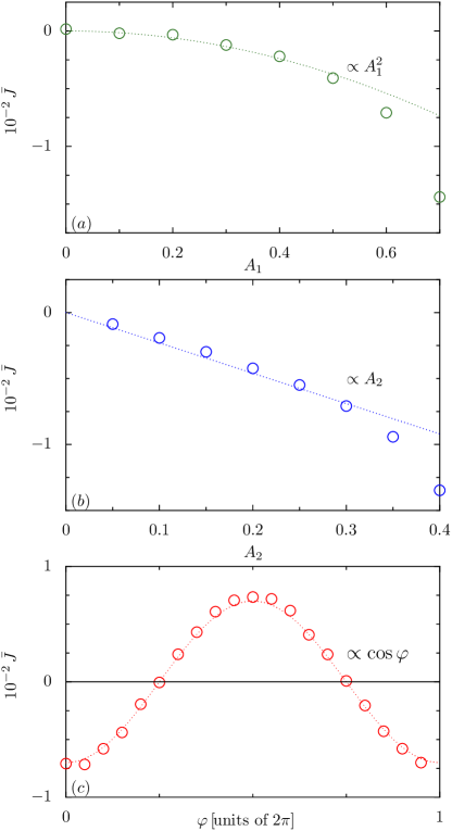
Figure 10: (Color-online) Ratcheting heat flux across a Lennard-Jones lattice. (a) Cycle averaged heat flux $\bar{J}$ vs. the fundamental driving amplitude $A_{1}$ with fixed $A_{2}=0.3$ and $\varphi=0$. (b) Cycle averaged heat flux $\bar{J}$ vs. the driving amplitude $A_{2}$ with fixed $A_{1}=0.6$ and $\varphi=0$. (c) Cycle averaged heat flux $\bar{J}$ vs. the phase shift $\varphi$ with fixed $A_{1}=0.6$ and $A_{2}=0.3$. For all cases, the lattice size is set as $N=50$ and the reference temperature is chosen as $T_{0}=3$.

Controlling heat flux via the phase shift $\varphi$

For single particle Brownian motors, it is well known that the directed transport in leading order of nonlinearity is proportional to the non-vanishing time-averaged third moment goychuk ; denisov . Whether this result still holds true for a spatially extended ratchet system can be tested in the present context numerically only. We conjecture that the directed current still will be proportional to the third order moment $\overline{(\Delta T(t)/2T_{0})^{3}}$, i.e. $\bar{J}\propto A_{1}^{2}A_{2}\cos{\varphi}$. The numerically evaluated heat flux $\bar{J}$ is depicted vs. $A_{1}$, $A_{2}$ and $\varphi$ in Fig. 10. As expected from theory, it is only for small values of driving amplitudes $A_{1}$ ($A_{1}<0.5$ in panel (a)) and $A_{2}$ ($A_{2}<0.3$ in panel (b)) that the heat current response $\bar{J}$ follows the theoretical scaling law $\bar{J}\propto A^{2}_{1}A_{2}$ with good accuracy. Note that the sign of the flux remains, however, undetermined from the form of harmonic mixing with opposite signs for $\pm A_{2}$. At larger driving strengths, higher order nonlinear contributions yield a sizable contribution, thus causing deviations from the leading scaling behavior. Interestingly enough, however, the heat current $\bar{J}$ is found to exhibit the dependence on the relative phase shift $\bar{J}\propto\cos{\varphi}$ very accurately, even for substantial large driving strengths; i.e. for $A_{1}=0.6$ see in Fig. 10(c). This numerical finding is advantageous for the control of heat current in spatially extended systems: the direction of directed heat flow can be reversed by merely adjusting the relative phase shift $\varphi$ of the second harmonic drive.

V Conclusions

In conclusion, we have demonstrated sizable shuttling of a net heat flux across 1D homogenous nonlinear lattices of the FPU-type and Lennard-Jones type by applying two different symmetry breaking mechanisms. These different mechanisms are imposed via temporal modulations of the bath temperature(s). For a modulation of temperature of one heat bath only a symmetric harmonic driving is sufficient to induce a non-vanishing heat flux. The resulting ratchet heat flux can be elucidated at low driving frequencies by virtue of an adiabatic estimate in terms of a single quadrature, see Eq. (9). The expression involves the knowledge of the nonlinear temperature dependent heat conductivity. According to this adiabatic analysis, in the linear transport regime, the ratchet heat flux is found to be proportional to the square of driving amplitude and does vanish in the thermodynamic limit $N\rightarrow\infty$.

For a situation with temperature modulations applied at both heat baths, a simple harmonic driving no longer induces a ratchet heat flux. If a second harmonic driving is included one can break the symmetry dynamically. The resulting ratchet heat flux obeys, however, no simple adiabatic estimate so that even the direction of the ratcheting heat flux cannot be predicted a priori. Moreover, we detect in the non-adiabatic regime a distinct reversal of heat flux for the case of the FPU-$\alpha\beta$ chain: It occurs around the thermal response time set by the anomalous heat conductivity. For the realistic situation with a Lennard-Jones lattice we find that the resulting flux of the Brownian heat motor is robust and is practically independent of system size.

Noteworthy is the fact that the directed heat flux is substantially larger for a physically realistic Lennard-Jones lattice as compared to the situation of coupled, non-identical Frenkel-Kontorova lattices, see in Ref. LHL . As a consequence, an experimental setup as put forward with this work seems more feasible to realize such a Brownian motor for shuttling heat as compared to a physical situation with two coupled Frenkel-Kontorova lattices.

- (1) L. Wang and B. Li, Physics World 21 (3), 28 (2008).
- (2) M. Terraneo, M. Peyrard, and G. Casati, Phys. Rev. Lett. 88, 094302 (2002).
- (3) B. Li, L. Wang, and G. Casati, Phys. Rev. Lett. 93, 184301 (2004).
- (4) D. Segal and A. Nitzan, Phys. Rev. Lett. 94, 034301 (2005).
- (5) B. Hu, L. Yang, and Y. Zhang, Phys. Rev. Lett. 97, 124302 (2006).
- (6) M. Peyrard, Europhys. Lett. 76, 49 (2006).
- (7) N. Yang, N. Li, L. Wang, and B. Li, Phys. Rev. B 76, 020301(R) (2007).
- (8) B. Li, L. Wang, and G. Casati, Appl. Phys. Lett. 88, 143501 (2006).
- (9) L. Wang and B. Li, Phys. Rev. Lett. 99, 177208 (2007).
- (10) L. Wang and B. Li, Phys. Rev. Lett. 101, 267203 (2008).
- (11) C. W. Chang, D. Okawa, A. Majumdar, and A. Zettl, Science 314, 1121 (2006).
- (12) P. Reimann, R. Bartussek, R. Häussler, and P. Hänggi, Phys. Lett. A 215, 26 (1996).
- (13) R. D. Astumian and P. Hänggi, Phys. Today 55 (11), 33 (2002).
- (14) P. Hänggi, F. Marchesoni, and F. Nori, Ann. Phys. (Leipzig) 14, 51 (2005).
- (15) P. Reimann and P. Hänggi, Appl. Phys. A 75, 169 (2002).
- (16) P. Hänggi and F. Marchesoni, Rev. Mod. Phys. 81, 387 (2009).
- (17) N. Li, P. Hänggi, and B. Li, EPL 84, 40009 (2008).
- (18) C. Van den Broeck and R. Kawai, Phys. Rev. Lett. 96, 210601 (2006).
- (19) D. Segal, A. Nitzan and P. Hänggi, J. Chem. Phys. 119, 6840 (2003).
- (20) D. Segal and A. Nitzan, Phys. Rev. E 73, 026109 (2006).
- (21) R. Marathe, A. M. Jayannavar and A. Dhar, Phys. Rev. E 75, 030103(R) (2007).
- (22) M. van den Broek and C. Van den Broeck, Phys. Rev. Lett. 100, 130601 (2008).
- (23) B. Hu, B. Li, and H. Zhao, Phys. Rev. E 57, 2992 (1998).
- (24) N. Li and B. Li, EPL 78, 34001 (2007).
- (25) S. Lepri, R. Livi, and A. Politi, Phys. Rep. 377, 1 (2003).
- (26) J. Luczka, R. Bartussek and P. Hänggi, Europhys. Lett. 31, 431 (1995).
- (27) P. Hänggi, R. Bartussek, P. Talkner, and J. Luczka, Europhys. Lett. 35, 315 (1996).
- (28) I. Goychuk and P. Hänggi, Europhys. Lett. 43, 503 (1998).
- (29) S. Flach, O. Yevtushenko, and Y. Zolotaryuk, Phys. Rev. Lett. 84, 2358 (2000).
- (30) S. Denisov, S. Flach, A.A. Ovchinnikov, O. Yevtushenko, and Y. Zolotaryuk, Phys. Rev. E 66, 041104 (2002).
- (31) P. Hänggi and F. Marchesoni, Rev. Mod. Phys. 81, 387 (2009); see Section II.C.1 therein.
- (32) H. Kaburaki and M. Machida, Phys. Lett. A 181, 85 (1993).
- (33) S. Lepri, R. Livi, A. Politi, Phys. Rev. Lett. 78, 1896 (1997).
- (34) A. Pereverzev, Phys. Rev. E 68, 056124 (2003).