Lyapunov instability of rough hard-disk fluids

Abstract

The dynamical instability of rough hard-disk fluids in two dimensions is characterized through the Lyapunov spectrum and the Kolmogorov-Sinai entropy, $h_{KS}$, for a wide range of densities and moments of inertia $I$. For small $I$ the spectrum separates into translation-dominated and rotation-dominated parts. With increasing $I$ the rotation-dominated part is gradually filled in at the expense of translation, until such a separation becomes meaningless. At any density, the rate of phase-space mixing, given by $h_{KS}$, becomes less and less effective the more the rotation affects the dynamics. However, the degree of dynamical chaos, measured by the maximum Lyapunov exponent, is only enhanced by the rotational degrees of freedom for high-density gases, but is diminished for lower densities. Surprisingly, no traces of Lyapunov modes were found in the spectrum for larger moments of inertia. The spatial localization of the perturbation vector associated with the maximum exponent however persists for any $I$.

I Introduction

The phase space trajectory of a many-body system with convex particles is Lyapunov unstable posch_hoover_1988 ; gaspard_1998 , which means that it is extremely sensitive to small (infinitesimal) perturbations of the initial conditions. If all possible perturbation vectors are represented as an infinitesimal hypersphere centered on and co-moving with a phase point, at later times this object is deformed under the action of the linearized flow. The main axes exponentially grow or shrink with time. The time-averaged rates are referred to as Lyapunov exponents, and the sorted set of exponents, $\{\lambda_{l},l=1\dots D\}$, as Lyapunov spectrum. Here, $D$ is the phase-space dimension. The relation of the Lyapunov spectrum to more familiar fluid properties has motivated much work over the last two decades. If, for example, the density of a soft-potential Weeks-Chandler-Anderson fluid WCA is isothermally increased from the fluid to the solid phase, the Kolmogorov-Sinai (dynamical) entropy, which is equal to the sum of all positive Lyapunov exponents Pesin , exhibits a maximum at a density which is about 20 % smaller than the liquid-line density at the fluid-to-solid phase transition. This result, which has been verified for two- forster_posch_2005 ; toxvaerd_1983 and three-dimensional phh_1990 ; heyes_2006 systems, is somewhat surprising. It implies that in soft-potential systems most efficient phase space mixing and information generation about the initial state does not occur at the transition itself but at a slightly smaller density. This sheds new light on our understanding of the onset of phase transitions. Another example concerns stationary non-equilibrium systems with time-reversible equations of motion. In this case, the Lyapunov spectrum may be directly linked with the transport coefficients and the rate of entropy production posch_hoover_1988 ; hoover_1999 .

Systematic studies of simple atomic fluids, such as hard-sphere and soft-sphere models, have revealed some interesting features. In particular, trajectory perturbations related to the largest (in absolute value) Lyapunov exponents are strongly localized in physical space hoover_posch_1998 ; FHPH_2004 ; TM_2003a . This means that at any instant of time only a very small fraction of all particles contributes to the fastest dynamical events responsible for the largest rates of perturbation growth (or decay). This localization also persists in the thermodynamic limit. A similar localization property for the maximum-exponent perturbations was found for one-dimensional distributed systems with space-time chaos pikovsky_1998 . On the other hand, perturbation vectors associated with the smallest (in absolute value) exponents may be delocalized and exhibit wave-like patterns in space. These so-called Lyapunov modes were first observed for systems of hard dumbbells MPH_1998 ; MP_2002 and hard disks PH_2000 ; TM_2003b ; EFPZ_2005 and are a consequence of the basic symmetries, namely invariance with respect to time and space translations (depending on the boundary conditions). Due to exponent degeneracies, they are recognized by a step-like appearance of the Lyapunov spectrum for small (in absolute value) exponents. For soft-potential systems, however, sophisticated Fourier transform techniques are required to demonstrate the presence of Lyapunov modes forster_posch_2005 ; RADONS .

The study of Lyapunov exponents has also been extended to simple molecular systems such as soft Borzsak_1996 ; Kum_1998 and hard dumbbells MPH_1998 ; MP_2002 in two dimensions. In this case the dynamics is affected by qualitatively different degrees of freedom, translation and rotation, which both have a pronounced effect on the spectrum.

In this paper we turn to a related model, which also incorporates the idea of the coupling of translational degrees of freedom to some internal energy, which affects the dynamics, namely rough hard disks in two dimensions. The three-dimensional version of this model, rough hard spheres, was first introduced by Bryan bryan:1894 in 1894, and was consecutively treated by Pidduck pidduck:1922 and, in particular, by Chapman and Cowling chapman:1953 , who worked out explicit formulas for the transport coefficients in terms of kinetic theory. It is an extension of the familiar smooth hard-sphere model, with angular momentum added to each sphere due to roughness. Roughness is introduced by the requirement that a collision between two particles reverses the relative surface velocity at the point of contact of the collision partners, exchanging both linear and angular momentum in the process. This definition corresponds to the maximum possible roughness between two particles. This model was extensively studied by Berne and co-workers with respect to various models of molecular rotational relaxation Berne_I . They also investigated the dynamical properties of models with partial roughness in between that of the smooth and the maximum rough sphere models Berne_II ; Berne_III , in particular the hydrodynamic long-time behavior of various correlation functions Berne_IV .

Here we are concerned with the two-dimensional version of this model with maximum roughness, $N$ identical rough hard disk in a box with periodic boundaries. The paper is organized as follows: In Section II we describe the model and derive the collision map for colliding particles and the respective linearized map for the dynamics in tangent space. All simulation results are presented in Section III. We conclude with a discussion of the results in Sec. IV.

II Rough hard sphere and hard disk models

Phase space dynamics

We consider the three-dimensional ($d=3)$ rough hard-sphere model first. It consists of $N$ identical hard spheres of diameter $\sigma$, mass $m$ and moment of inertia $I$, which are located at positions $\vec{q}_{i}$, and which move with (linear) velocities $\vec{v}_{i}$ and rotate with angular velocities $\vec{\omega}_{i}$, $i\in\{1,\cdots,N\}$. Due to the isotropy of the spheres, the particle orientation is not required in the following, and the state vector is given by

$$\vec{\Gamma}=\Big{(}\{\vec{q}_{i}\},\{\vec{v}_{i}\},\{\vec{\omega}_{i}\}\Big{)}.$$ (1)

The phase space dynamics is characterized by force-free ”streaming”, interrupted by instantaneous pairwise collisions, at which momentum and angular momentum are transferred between the colliding particles, such that the relative surface velocity $\vec{g}$ at the point of contact of the two particles is reversed. Their positions are not affected by the collisions.

The equations of motion for the streaming between binary collisions is written as a system of first-order differential equations,

$$\dot{\vec{\Gamma}}=\vec{F}(\vec{\Gamma}):\;\;\Big{(}\{\dot{\vec{q}}_{i}=\vec{v}_{i}\},\{\dot{\vec{v}}_{i}=\vec{0}\},\{\dot{\vec{\omega}}_{i}=\vec{0}\}\Big{)},$$ (2)

where $i=1,\dots,N$. It has an obvious solution.

At a collision between two particles $i$ and $j$, the collision map

$$\vec{\Gamma}\,^{\prime}=\vec{M}(\vec{\Gamma})$$ (3)

is introduced, which relates the pre-collision state $\vec{\Gamma}$ to the post-collision state $\vec{\Gamma}\,^{\prime}$. With the following definitions,

$$\vec{q}=\vec{q}_{j}-\vec{q}_{i};\;\;\;\vec{n}=\frac{1}{\sigma}\vec{q};\;\;\;\vec{v}=\vec{v}_{j}-\vec{v}_{i};\;\;\;\vec{\Omega}=\vec{\omega}_{j}+\vec{\omega}_{i},$$ (4)

the relative surface velocity at the point of contact of $i$ and $j$ becomes

$$\vec{g}=\vec{v}+\frac{\sigma}{2}\,\vec{n}\times\vec{\Omega}.$$ (5)

Here, $\vec{n}$ denotes a unit vector along the line of centers from $i$ to $j$ at the instant of collision, and $\vec{v}$ is the respective relative velocity. Maximum roughness requires that

$$\vec{g}\,^{\prime}=-\vec{g},$$ (6)

where the prime, here and below, refers to the state immediately after the collision. Together with the conservation laws for energy, linear momentum and angular momentum, that part of the collision map relevant for the collision between particles $i$ and $j$ becomes chapman:1953

$$\vec{q}_{i}\,^{\prime} = \vec{q}_{i},$$

$$\vec{q}_{j}\,^{\prime} = \vec{q}_{j},$$

$$\vec{v}_{i}\,^{\prime} = \vec{v}_{i}+\gamma\vec{g}+\beta\,\vec{n}(\vec{n}\cdot\vec{v}),$$

$$\vec{v}_{j}\,^{\prime} = \vec{v}_{j}-\gamma\vec{g}-\beta\,\vec{n}(\vec{n}\cdot\vec{v}),$$ (7)

$$\vec{\omega}_{i}\,^{\prime} = \vec{\omega}_{i}+(2\beta/\sigma)\,\vec{n}\times\vec{g},$$

$$\vec{\omega}_{j}\,^{\prime} = \vec{\omega}_{j}+(2\beta/\sigma)\,\vec{n}\times\vec{g}.$$

Here, $\beta$ and $\gamma$ are constants, which depend on the moment of inertia $I$ around a diameter of the sphere:

$$\kappa=\frac{4I}{m\sigma^{2}};\qquad\gamma=\frac{\kappa}{\kappa+1};\qquad\beta=\frac{1}{\kappa+1}.$$ (8)

The dimensionless parameter $\gamma$ controls the coupling between translational and rotational degrees of freedom. In the limit $I\rightarrow 0$, the translational and rotational degrees of freedom decouple and the rough hard sphere model reduces to the conventional smooth hard-sphere model without roughness DPH_1996 , if all angular velocity vectors are discarded.

Tangent space dynamics

A perturbed trajectory is separated from the reference trajectory by an offset vector

$$\vec{\delta\Gamma}=(\{\vec{\delta q}_{i}\},\{\vec{\delta v}_{i}\},\{\vec{\delta\omega}_{i}\}),$$ (9)

which evolves during the streaming phase according to the linearized equations of motion

$$\dot{\vec{\delta\Gamma}}=\frac{\partial\vec{F}}{\partial\vec{\Gamma}}\cdot\vec{\delta\Gamma}:\Big{(}\{\dot{\vec{\delta q}}_{i}=\vec{\delta v}_{i}\},\{\dot{\vec{\delta v}}_{i}=\vec{0}\},\{\dot{\vec{\delta\omega}}_{i}=\vec{0}\}\Big{)},$$ (10)

$i=1,\cdots,N$. It is trivially solved.

The linearization of the collision map (3) is obtained from Ref. DPH_1996 :

$$\vec{\delta\Gamma}\,^{\prime}=\frac{\partial\vec{M}}{\partial\vec{\Gamma}}\cdot\vec{\delta\Gamma}+\left[\frac{\partial\vec{M}}{\partial\vec{\Gamma}}\cdot\vec{F}(\vec{\Gamma})-\vec{F}\left(\vec{M}(\vec{\Gamma})\right)\right]\delta\tau_{c}.$$ (11)

Here, $\delta\tau_{c}$ is the (infinitesimal) time shift between the collision of the reference trajectory and of the perturbed trajectory, which may be positive or negative. Similarly, we denote by $\delta\vec{q}_{c}$ the shift in configuration space of the collision points of these two trajectories. If, as before, $i$ and $j$ are the colliding particles, these quantities are computed from DP_1997

$$\delta\tau_{c}=-\frac{\delta\vec{q}\cdot\vec{n}}{\vec{v}\cdot\vec{n}};\qquad\delta\vec{q}_{c}=\delta\vec{q}+\vec{v}\,\delta\tau_{c},$$ (12)

where we use a notation for the perturbed quantities which is analogous to the previous notation in phase space (see Eq. (4)):

$$\delta\vec{q}=\delta\vec{q}_{j}-\delta\vec{q}_{i};\;\;\;\;\delta\vec{v}=\delta\vec{v}_{j}-\delta\vec{v}_{i};\;\;\;\;\delta\vec{\Omega}=\delta\vec{\omega}_{j}+\delta\vec{\omega}_{i}.$$ (13)

Since $\vec{\delta q}_{c}=\sigma\vec{\delta n}$, we also find from Eq. (5):

$$\delta\vec{g}=\delta\vec{v}+\frac{1}{2}\Big{[}\delta\vec{q}_{c}\times\vec{\Omega}+\vec{q}\times\delta\vec{\Omega}\Big{]}.$$ (14)

With this notation, we obtain for that part of the linearized map (11) belonging to the collision of $i$ and $j$:

$$\delta\vec{q}_{i}\,^{\prime} = \delta\vec{q}_{i}-\Big{[}\gamma\vec{g}+\frac{\beta}{\sigma^{2}}\vec{q}(\vec{q}\cdot\vec{v})\Big{]}\delta\tau_{c}\,,$$

$$\delta\vec{q}_{j}\,^{\prime} = \delta\vec{q}_{j}+\Big{[}\gamma\vec{g}+\frac{\beta}{\sigma^{2}}\vec{q}(\vec{q}\cdot\vec{v})\Big{]}\delta\tau_{c}\,,$$

$$\delta\vec{v}_{i}\,^{\prime} = \delta\vec{v}_{i}+\gamma\,\delta\vec{g}$$

$$+\frac{\beta}{\sigma^{2}}\Big{[}\delta\vec{q}_{c}(\vec{q}\cdot\vec{v})+\vec{q}(\vec{v}\cdot\delta\vec{q}_{c})+\vec{q}(\vec{q}\cdot\delta\vec{v})\Big{]}\,,$$

$$\delta\vec{v}_{j}\,^{\prime} = \delta\vec{v}_{j}-\gamma\,\delta\vec{g}$$

$$-\frac{\beta}{\sigma^{2}}\Big{[}\delta\vec{q}_{c}(\vec{q}\cdot\vec{v})+\vec{q}(\vec{v}\cdot\delta\vec{q}_{c})+\vec{q}(\vec{q}\cdot\delta\vec{v})\Big{]}\,,$$

$$\delta\vec{\omega}_{i}\,^{\prime} = \delta\vec{\omega}_{i}+\frac{2\beta}{\sigma^{2}}\Big{[}\delta\vec{q}_{c}\times\vec{g}+\vec{q}\times\delta\vec{g}\Big{]}\,,$$

$$\delta\vec{\omega}_{j}\,^{\prime} = \delta\vec{\omega}_{j}+\frac{2\beta}{\sigma^{2}}\Big{[}\delta\vec{q}_{c}\times\vec{g}+\vec{q}\times\delta\vec{g}\Big{]}.$$ (15)

If the moment of inertia vanishes ($\gamma\to 0$ and $\beta\to 1$), the linearized collision map of the smooth hard sphere fluid is recovered DP_1997 , if the angular velocity perturbations are discarded.

Computer simulations of hard disks in two dimensions

For the remainder of this work we restrict ourselves to the case of planar rough disks on the $xy$ plane, $d=2$. All the equations above remain valid in this case, if all position and velocity vectors are placed in the $xy$ plane, and all angular velocity vectors $\vec{\omega}_{i}$ are perpendicular to this plane with a single non-vanishing $z$ component $\omega_{i}$. Discarding all superfluous components, we are left with $D=5N$ components for the state vector $\vec{\Gamma}$ and for any perturbation vector $\vec{\delta\Gamma}$.

Depending on the mass distribution of the disks and, hence, their moment of inertia $I$ with respect to a perpendicular axis through the center, the coupling parameter $\kappa$ may take values between zero and one: $\kappa=0$ applies, if all the mass is located in the center, $\kappa=1/2$ corresponds to a uniform mass distribution, and $\kappa=1$ is obtained, if all the mass is concentrated on the perimeter of the disk.

For our numerical work we use reduced units, for which the disk diameter $\sigma$, its mass $m$, and the Boltzmann constant $k$ are set to unity. The time-averaged translational kinetic energy per particle, $\langle K\rangle/N=\sum_{i}m\langle\vec{v}_{i}\cdot\vec{v}_{i}\rangle/(2N)$ is taken as the unit of energy. Thus the temperature is one, $T=1$, as in our previous work on smooth hard disks, which facilitates comparison DPH_1996 . We have ascertained that the translational and rotational temperatures agree. The unit of time is $(m\sigma^{2}N/\langle K\rangle)^{1/2}$. Lyapunov exponents and the Kolmorov-Sinai entropy are measured in units of $\sqrt{kT/m\sigma^{2}}$. The number density is defined as $\rho=N\sigma^{2}/V$, where $N$ is the total number of disks, and $V$ denotes the area of the simulation box with extensions $L_{x},L_{y}$. For fluid phases we take a square box, $L_{x}=L_{y}$, where the particles are initially put on a square lattice with random velocities and random angular velocities. For solid phases the aspect ratio $L_{y}/L_{x}=\sqrt{3}/2$ is used, which is compatible with the triangular close-packed lattice and does not differ much from a square. By initially putting the particles on a triangular lattice with random velocities and angular velocities, high density systems up to the close-packed density $\rho_{0}=1.1547$ may be studied in this way. Periodic boundary conditions are used throughout. The only free parameters are the number density $\rho$ and the moment of inertia $I$ (respective the coupling parameter $\kappa=4I$).

To evolve the system, an event-driven algorithm similar to that of Rapaport Rapaport was used. Proper care was taken to avoid missing glancing collisions. The conservation of energy and linear momentum was carefully verified. The total angular momentum is not conserved due to the periodic boundaries. For the computation of the $5N$ Lyapunov exponents, the classical algorithm of Benettin et al. Benettin and Shimada et al. Shimada , properly modified for the instantaneous elastic rough collisions encountered here, was used. Simultaneously with the reference trajectory $\vec{\Gamma}(t)$, $5N$ replica of perturbation vectors, $\vec{\delta\Gamma}^{(l)}(t),\;l=1,\cdots,5N$, with orthonormal initial conditions were evolved and periodically re-orthonormalized with a Gram-Schmidt procedure DPH_1996 ; DP_1997 .

III Results

Lyapunov spectra

In this section we discuss the Lyapunov spectra of rough disk fluids and solids. A full spectrum consists of the ordered set of Lyapunov exponents, $\lambda_{1}\geq\lambda_{2}\geq\cdots\geq\lambda_{D}$, where $D$ is the phase space dimension. For a symplectic system as in our case, the Lyapunov exponents always appear in pairs with a vanishing pair sum. Therefore, the Lyapunov spectrum consists of a positive and a negative branch and is symmetric, $\lambda_{l}=-\lambda_{D+1-l}$, if plotted as a function of the index $l$. In the absence of magnetic fields, this so-called ”conjugate pairing symmetry” may simply be viewed as a consequence of the time-reversibility of the dynamical equations. Therefore, we may restrict ourselves to the positive branch of the spectrum, $1\leq l\leq D/2$, for which $\lambda_{l}\geq 0$, which considerably reduces the computational effort. Examples for full spectra will be given below (see the upper panel of Fig. 8).

Another important property concerns the vanishing exponents, which are a consequence of the fundamental continuous symmetries which leave the Lagrangian and, hence, the motion equations invariant. According to Nöther’s theorem, each such symmetry corresponds to a constant of the motion Scheck and, in addition, generates two symplectic-conjugate vector fields in phase space, along which perturbations do not stretch or shrink and, therefore, give rise to two vanishing exponents gaspard_1998 . For example, invariance with respect to time translation gives rise to energy conservation and to two vanishing exponents. Similarly, invariance with respect to uniform translation in space gives rise to momentum conservation and four more vanishing exponents. However, isotropy of space and, hence, angular momentum conservation applies locally for each collision, but not globally due to the periodic boundary conditions. Altogether only 6 Lyapunov exponents vanish in our case, as is also confirmed by the simulations.

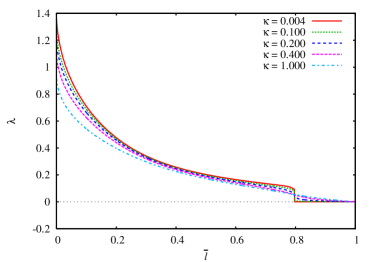
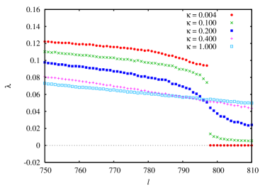
Figure 1: (Color online) Lyapunov spectra for a system of $N=400$ rough hard disks at a low density $\rho=0.1$. The various curves are for different moments of inertia $I$, where the keys refer to the coupling parameter $\kappa=4I$. The uniform mass distribution corresponds to $\kappa=0.5$. Top panel: Positive branches of the specta. The reduced index $\bar{l}$ is used on the abscissa. Bottom: Magnification of the transition region between translation and rotation dominated exponents. The un-normalized index $l$ is used on the abscissa.

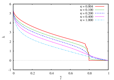
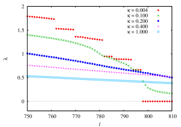
Figure 2: (Color online) Lyapunov spectra for a system of $N=400$ rough hard disks at a moderately high density $\rho=0.7$ (top). The various curves are for different moments of inertia, where the keys specify the coupling parameter $\kappa=4I$. The uniform mass distribution corresponds to $\kappa=0.5$. Top panel: Positive branches of the specta. The reduced index $\bar{l}$ is used on the abscissa. Bottom panel: Magnification of the transition region between translation and rotation dominated exponents. The un-normalized index $l$ is used on the abscissa. Reduced units and periodic boundaries are used as explained in the main text.

Although a spectrum only consists of discrete points indexed by the integer $l$ – or by the reduced index $\bar{l}=2l/D$ - most of the time in the figures below it is represented by a smooth line drawn through these points to enhance the clarity.

To assess the influence of translation-rotation coupling on the Lyapunov spectra, we show in Fig. 1 results for a rather dilute gas, $\rho=0.1$, of $N=400$ rough disks at a temperature $T=1$. The various curves belong to different moments of inertia $I$ and are specified by their coupling parameters $\kappa=4I$. The system is fairly large, and the results are close to the thermodynamic limit DPH_1996 . The phase space has $D=2000$ dimensions. In the top panel of Fig. 1 the positive branches of the full spectra are shown, where the normalized index $\bar{l}=l/(D/2)$ is used ($1\leq l\leq D/2=1000$) on the abscissa. Most noticeable is the transition region near $\bar{l}_{0}=(2N-3)/(D/2)=0.797$, which separates the specta into a translation-dominated regime for $\bar{l}\leq\bar{l}_{0}$ and a rotation-dominated regime for $\bar{l}_{0}<\bar{l}\leq(5N-6)/D)$. A magnification of the transition region is shown in the lower panel of Fig. 1, where the un-normalized index $l$ is used on the horizontal axis. Analogous spectra for a rather dense gas, $\rho=0.7$, are shown in Fig. 2.

For very small $\kappa$ translation and rotation are effectively decoupled and the dynamics is almost identical to that of a smooth hard-disk gas. For 400 particles the positive exponents $\lambda_{1},\cdots,\lambda_{797}$ agree with the positive exponents of the smooth hard disks and, hence, are translation dominated, whereas the (very small but positive) exponents $\lambda_{798},\cdots\lambda_{997}$ are due to the angular velocity perturbations and are only present in the rough-disk case. The three remaining exponents, $\lambda_{998},\cdots,\lambda_{1000}$, vanish due to the conserved quantities. Note that this is only the positive branch of the full spectrum.

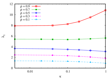
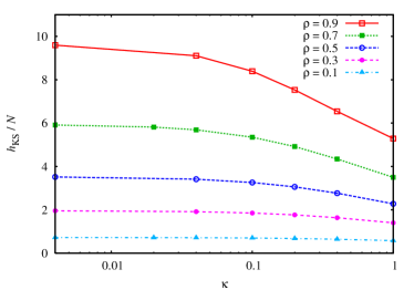
Figure 3: (Color online) Dependence of the maximum Lyapunov exponent $\lambda_{1}$ (upper panel) and of the Kolmogorov-Sinai entropy per particle, $h_{KS}/N$, (lower panel) on the coupling parameter $\kappa$ for various densities as indicated by the keys. The rough disk fluid contains N=400 particles and has (translational) temperature $kT=1$. Reduced units are used throughout.

The maximum Lyapunov exponent $\lambda_{1}$ is generally taken as in indicator and a measure for dynamical chaos. Similarly, the Kolmogorov-Sinai (or dynamical) entropy $h_{KS}$ is a measure of phase-space mixing DP_1997a . Due to the exponential instability, a number of initially close phase points are eventually uniformly distributed over the energy surface. The characteristic time for this mixing process is the mixing time $1/h_{KS}$ Krylov ; Zaslavsky . Since, according to Pesin Pesin , $h_{KS}$ is equal to the sum of the positive exponents, it is directly accessible through the Lyapunov spectrum. In the upper panel of Fig. 3 the maximum exponent as a function of $\kappa$ is shown for various densities. An analogous plot for the KS-entropy per particle, $h_{KS}/N$, is provided in the lower panel of the same figure. If $\kappa$ is increased, $\lambda_{1}$ decreases - weakly - for lower densities, $\rho<0.7$, and increases for large densities. The KS-entropy always decreases with $\kappa$, even for large densities. This means that mixing becomes less effective the more the rotational degrees of freedom affect the translational dynamics. Similarly, chaos is slightly reduced with increasing $\kappa$, at least for low-density gases.

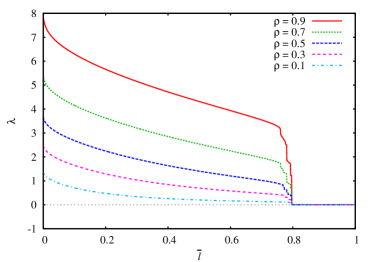
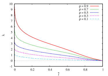
Figure 4: (Color online) Lyapunov spectra (positive branch only) of 400 rough hard disks with very small moment of inertia ($\kappa=4I=0.004$, upper panel) and with a large moment of inertia ($\kappa=0.4$, lower panel) for various densities as specified by the key. The reduced index $\bar{l}$ is used on the abscissa.

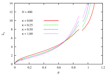
Figure 5: (Color online) Density dependence of the maximum exponent of 400 rough hard disks for various moments of inertia corresponding to the specified values of $\kappa$.

To demonstrate the density dependence, we show in the upper panel of Fig. 4 Lyapunov spectra for various densities of a 400-particle gas of hard disks with a very small moment of inertia for which $\kappa=0.004$. Analogous spectra with a large moment of inertia corresponding to $\kappa=0.4$ are provided in the lower panel of the same figure. All exponents increase with the density, in particular $\lambda_{1}$, as is shown in more detail in Fig. 5. where the maximum exponent - for various $\kappa$ - is plotted as a function of $\rho$. In some sense, $\lambda_{1}$ behaves similar to the potential-generated contribution to the pressure $P$ FMP_2004 . For low densities, both $(P/\rho kT)-1$ and $\lambda_{1}$ are proportional to the single particle collision frequency $\nu_{2}$. Fig. 5 resembles the respective phase diagram for the pressure. The conspicuous gap in the spectra marks the two-phase region for the fluid-solid transition. As mentioned in the previous section, the data beyond the solid line were obtained with a non-square simulation box (aspect ratio $\sqrt{3}/2$), the data below the fluid line with a square simulation box. This choice of aspect ratios merely facilitates the setting up of the initial conditions for the solid-state simulations and does not have any significance for the results. The gap disappears completely, if $\lambda_{1}$ is plotted as a function of the single-particle collision frequency $\nu_{2}$ (not shown), which is easily obtained from the simulation. This has been noted already for the smooth hard-disk system ($\kappa=0$) DPH_1996 and is also true for all $\kappa>0$. This means that the statistical distributions for the parameters characterizing the collisions (such as the impact parameter) do not noticeably differ for the disordered fluid and the coexisting crystal.

Based on kinetic theory, a density expansion for $\lambda_{1}$ of the smooth hard disk model ($\kappa=0$) becomes

$$\lambda_{1}=A\nu_{2}\left[-\ln\rho-B+{\cal O}(1/\ln\rho)\right],$$ (16)

where

$$\nu_{2}=2\pi^{1/2}\rho\sigma\left(kT/m\right)g(\sigma)$$ (17)

is the single-particle collision frequency. The pair distribution function at contact, $g(\sigma)$, converges to unity in the low-density limit. Estimates for the constants $A$ and $B$ have been computed by van Zon and van Beijeren, $A=1.473,B=2.48$ vZ1 ; vZ2 , which represent the numerical data well for very small densities $\rho<10^{-3}$. Expressions such as Eq. 16 with different constants are expected to hold also for the rough disks when $\kappa>0$.

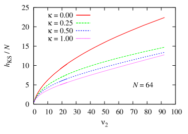
Figure 6: (Color online) Dependence of the Kolmogorov-Sinai entropy $h_{KS}$ on the single-particle collision frequency $\nu_{2}$ of $N=64$ rough disks for various $\kappa$ as indicated by the keys. $\nu_{2}$ is obtained by dividing the experimentally determined total number of collisions by $N/2$.

Whereas all of the results so far are for systems containing 400 particles, the dependence of the KS-entropy on the single-particle collision frequency $\nu_{2}$ is demonstrated in Fig. 6 for a system with only $N=64$ disks (to reduce the computational cost). This number is still large enough to be representative for large systems. As was found for the maximum Lyapunov exponent, the phase transition (near $\nu_{2}\approx 20$) does not specifically show up in $h_{KS}$ when viewed as a function of $\nu_{2}$ instead of $\rho$. If $\rho$ approaches the close-packed density $\rho_{0}=1.1547$, both $\lambda_{1}$ and $h_{KS}$ diverge due to the divergence of $\nu_{2}$. For very low densities and smooth hard disks ($\kappa=0$), a kinetic-theory based density expansion for the KS-entropy similar to that in Eq. 16 becomes vB_1997 ; vZ1

$$h_{KS}/N=A^{\prime}\nu_{2}\left[-\ln\rho+B^{\prime}+{\cal O}(\rho)\right].$$ (18)

Estimates for the constants $A^{\prime},B^{\prime}$ have been obtained by van Zon et al. vZ1 and most recently by de Wijn Astrid , $A^{\prime}=0.5,B^{\prime}=1.47\pm 0.11$, which describe the numerical data well for $\rho<10^{-3}$. Again we expect a similar representation to hold also for $\kappa>0$. Still, it seems surprising that the KS-entropy is reduced so much by the introduction of an internal degree of freedom (rotation), which effectively acts as energy storage in between collisions.

An interesting step-like structure is observed for very small $\kappa$ in Fig. 2 and in the upper panel of Fig. 4. These steps are a remnant of the degeneracy of exponents due to the existence of Lyapunov modes for smooth ($\kappa\equiv 0$) hard disk systems PH_2000 ; EFPZ_2005 . Lyapunov modes are periodic spatial perturbations associated with the small positive exponents with indices $l<l_{0}=2N-3$ (and with the conjugately paired negative exponents). The corresponding perturbation vectors may be represented as periodic vector fields coherently spread out over the simulation box and with well defined wave vectors. They may be understood as Goldstone modes of a system with continuous symmetries Goldstone - translation invariance in space and time - which give rise to conservation of energy and linear momentum Scheck and in addition to the six vanishing exponents gaspard_1998 . Note that angular momentum is globally not conserved according to the periodic boundaries and does not contribute. Fig. 2 shows that the exponent degeneracy and, hence the Lyapunov modes are still rather well developed for $\kappa=0.004$ corresponding to a moment of inertia $I=0.001$. This is independent of the density as is shown in the upper panel of Fig. 4. However, if $\kappa$ is increased, the steps quickly disappear and Lyapunov modes do not seem to exist any more. This is most clearly demonstrated in Fig. 2. It is not clear to us why this happens in view of the fact that modes are readily found for two-dimensional hard dumbbell fluids. Fourier transformation techniques will be required to settle this point.

For rough hard disks the angular velocity subspace of the full phase space has $N$ dimensions and contributes $N$ exponents to the full spectrum. For small $\kappa$ these exponents are different from zero, but small. Half of them belong to the positive branch (to which we restrict ourselves without loss of generality) and are located in the index interval $2N-2\leq l\leq(5N/2)-3$, sandwiched between the translation-dominated regime, $l\leq 2N-3$, and the three vanishing exponents still attributed to the positive branch, $(5N/2)-2\leq l\leq 5N/2$. We refer to this regime as rotation dominated. If $\kappa$ is increased, the exponents in this regime are increased, and the exponents in the translation dominated regime become smaller, until the spectrum becomes very uniform as, for example, in the lower panel of Fig. 4, and the separation into translation and rotation dominated regimes becomes meaningless. Such a system we call fully coupled. Translation and rotation contribute indistinguishably to the mixing process in phase space.

Localization of tangent-space perturbations

The maximum (minimum) Lyapunov exponent is the rate constant for the fastest growth (decay) of a phase-space perturbation and is dominated by the fastest dynamical events, binary collisions. It is not too surprising that the associated tangent vector components are significantly different from zero for only a few strongly-interacting particles at any instant of time. Thus, the respective perturbations are strongly localized in physical space. It has been shown that for both hard and soft disk respective sphere systems the localization persists in the thermodynamic limit, such that the fraction of tangent-vector components contributing to the generation of $\lambda_{1}$ follows a power law $\propto N^{-\eta},\eta>0$, and converges to zero for $N\to\infty$ MP_2002 ; PF_2002 ; FHPH_2004 ; forster_posch_2005 . The localization becomes gradually worse for larger indices $l>1$, until it ceases to exist and (almost) all particles collectively contribute to the coherent Lyapunov modes mentioned in the previous section. Similar observations for spatially extended systems have been made by various authors Manneville ; LR_1989 ; FMV_1991 ; TM_2003a ; TM_2003b .

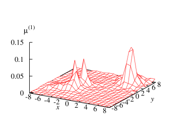
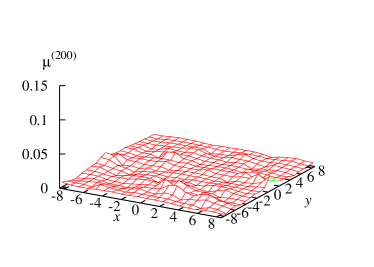
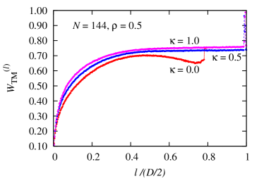
Figure 7: (Color online) Top: Instantaneous view of the action probability $\mu_{i}^{(1)}$ for the maximally localized tangent vector, plotted as a scalar field over the simulation box. For the grid interpolation a weight function $w(r)\propto r^{-2}$ is used, where $r$ is the distance of a particle to the grid point. The system consists of $N=144$ rough hard disks with $\kappa=0.5$ at a density $\rho=0.5$.
Middle: As in the top panel, but for $\mu_{i}^{(200)}$, which belongs to a delocalized vector with normalized index $\bar{l}=0.556$.
Bottom: Localization width $W_{TM}^{(l)}$ (see Eq. (19)) for $N=144$ disks with $\kappa$ indicated by the labels. The density $\rho=0.5$. The reduced index $\bar{l}=l/(D/2)$ is used on the abscissa, and $D=5N$.

To demonstrate the localization property of the rough hard-disk system, we define the contribution of an individual disk $i$ to the perturbation vector ${\vec{\delta}\Gamma}^{(l)}$ belonging to $\lambda_{l}$ as the square of the projection of ${\vec{\delta}\Gamma}^{(l)}$ onto the subspace of this disk,

$$\mu_{i}^{(l)}=\Big{(}\vec{\delta q_{i}}^{(l)}\Big{)}^{2}+\Big{(}\vec{\delta v_{i}}^{(l)}\Big{)}^{2}+\Big{(}\delta\omega_{i}^{(l)}\Big{)}^{2}.$$

Because ${\vec{\delta}\Gamma}^{(l)}$ is normalized in the Gram-Schmidt step of the algorithm, one has $\sum_{i}^{N}\mu_{i}^{(l)}=1$ for all $l$, and $\mu_{i}^{(l)}$ may be interpreted as a kind of (normalized) action probability of $i$ for the perturbation $l$. It should be noted that for the definition of $\mu_{i}^{(l)}$ the Euclidean norm is used and that all localication measures depend on this choice. Qualitatively, this is sufficient to demonstrate localization.

In the top panel of Fig. 7, $\mu_{i}^{(1)}$ for $l=1$ is plotted as a scalar field $\mu^{(1)}(\vec{q})$, where the surface is interpolated over regular grid points covering the whole simulation box. There exist one big and a few smaller competing active zones, which move around randomly such that the system remains homogeneous when viewed over a long time. This should be contrasted with the middle panel, where an analogous plot (with the same scale) is shown for the delocalized tangent vector with an index $l=200$ $(\bar{l}=0.556).$ For this comparison, the system contains 144 rough disks with $\kappa=0.5$ at a density $\rho=0.5.$

A number of localization measures have been introduced to assess the localization of ${\vec{\delta}\Gamma}^{(l)}$, not only for $l=1$ MP_2002 but for all $l$ TM_2003a ; TM_2003b . The most common is due to Taniguchi and Morriss TM_2003a , who define a ”localization width”

$$W_{TM}^{(l)}=\exp[S^{(l)}]/N,$$ (19)

which is based on the Shannon entropy for the ”probability” distribution $\mu_{i}^{(l)}$:

$$S^{(l)}=\left\langle-\sum_{i=1}^{N}\mu_{i}^{(l)}\ln\mu_{i}^{(l)}\right\rangle.$$

Here, $\langle\cdots\rangle$ denotes a time average. $W_{TM}^{(l)}$ is bounded according to $1/N\leq W_{TM}^{(l)}\leq 1$, where the lower and upper bounds apply for complete localization and delocalization, respectively. In the bottom panel of Fig. 7 we plot $W_{TM}^{(l)}$ for the 144-disk system used before. The value of $\kappa$ is indicated by the labels. This localization spectrum changes surprisingly little when $\kappa$ is increased from zero to one. The only major difference is for the rotation-dominated regime. For the smooth disks, $\kappa=0$, the points for $W_{TM}^{(l)}$ are irrelevant in this regime, $0.8\leq\bar{l}\leq 1.2$, and are not shown. Note that only data for the positive branch of the Lyapunov spectrum are shown, $\bar{l}\leq 1$.

Alternatively, an even simpler definition may be used, which involves the Fermi entropy (sometimes also referred to as the quadratic entropy), Jumarie

$$S_{F}^{(l)}=\left\langle\sum_{i=1}^{N}\mu_{i}^{(l)}(1-\mu_{i}^{(l)})\right\rangle.$$ (20)

It has the desired property: $S_{F}^{(l)}$ vanishes, if only a single particle is responsible for the phase-space growth (extreme localization), it is $(N-1)/N\approx 1$, if all particles contribute identically (complete coherent delocalization), and it is in between otherwise. This measure might be particularly useful, whenever localization is even more complete than in the case presented here, but it distinguishes poorly between very delocalized states..

At this point, a critical remark is in order. The localization spectrum in the bottom panel of Fig. 7 is shown for the positive branch of the Lyapunov spetrum only. It should be completely symmetrical with respect to the conjugate negative branch, $S^{(l)}=S^{(D+1-l)}$, due to the time reversible phase-space structure: a time reversal operation converts the stable manifold into the unstable manifold and vice versa. For the smooth hard-disk case, $\kappa=0$, this symmetry is observed with high numerical precision JvM_2005 ; BP_2009 . However, for $\kappa>0$ the spectra are slightly asymmetric (not shown). The reason for this asymmetry is subtle. The perturbation vectors ${\vec{\delta}\Gamma}^{(l)}$ we use in this work are ortho-normal. They span the correct subspaces of the tangent space required for the computation of the Lyapunov exponents according to the standard algorithm Benettin ; Shimada ; EFPZ_2005 , but they are not covariant: that means, they do not strictly follow the linearized dynamics in tangent space, but are regularly re-orthonormalized by the Gram-Schmidt procedure. As a consequence, they are not invariant under time reversal. The last property, however, is required for a complete symmetry of the localization spectrum, such that the expanding vector ${\vec{\delta}\Gamma}^{(l)}$ in the time-forward direction becomes the contracting vector ${\vec{\delta}\Gamma}^{(D+1-l)}$ in the time-backward direction. If proper covariant Lyapunov vectors Ginelli are used instead of the Gram-Schmidt vectors, the symmetry is re-established for $\kappa>0$. Details will be communicated in a forthcoming publication BP_2009 .

Convergence times in tangent space

For the Lyapunov exponents to converge, the orthonormal set of tangent vectors needs to reach its proper orientation in tangent space starting from an arbitrary initial orientation. The convergence time varies with the number of particles and with the index $l$. For smooth particle systems it was shown in Ref. DHP_2002 that the vector associated with the maximum exponent aligns with a convergence time proportional to $N^{\alpha}$, where $\alpha$ lies between 0.4 (for smooth hard disks) and 0.9 (for soft repulsive interaction potentials). For higher indices the convergence is an even slower collective phenomenon. In this section the methods of Ref. DHP_2002 are adapted to determine the system-size dependence of the convergence times of rough disks not only for $l=1$ but for all tangent vectors.

We consider $M$ randomly oriented orthonormal sets of tangent vectors, $\Delta_{m}=\{\vec{\delta\Gamma}_{m}^{(l)}\},l=1,\cdots,D$, where $m=1,\cdots,M$. Each set spans the full $D$-dimensional tangent space and acts as an initial condition for the computation of a full Lyapunov spectrum for the same reference trajectory. All spectra eventually converge. Any two tangent vectors giving rise to the same Lyapunov exponent but belonging to different initial sets $\Delta$ need to become parallel or anti-parallel in the course of time, such that their dot-product approaches $\pm 1$. To measure the convergence time for a given $l$, we average over all such possible products,

$$\chi_{l}(t)=\frac{2}{M(M-1)}\sum_{m=1}^{M-1}\sum_{m^{\prime}=m+1}^{M}\left|\vec{\delta\Gamma}_{m}^{(l)}\cdot\vec{\delta\Gamma}_{m^{\prime}}^{(l)}\right|.$$ (21)

$\chi_{l}(t)$ increases with time from $\chi_{0}$ to unity, where the initial value ($\chi_{0}\approx 0.06$ for $N=36$) is independent of $l$ due to the random orientation of the sets $\Delta$ and converges to zero for $N\to\infty$. The time for which $\chi_{l}(t)$ crosses a threshold $\Theta$ for the first time is taken as a measure of the convergence time $\tau_{l}$. In the following we take $\Theta=0.9$. Any other choice for this threshold only results in times which differ by a constant factor.

Before continuing the discussion, we note that the Lyapunov spectrum exists in the thermodynamic limit. This has been shown for smooth hard disks and hard spheres DPH_1996 and means that for $N\to\infty$, at constant density, the Lyapunov spectra quickly converge to a limiting curve when plotted as a function of the reduced index $\bar{l}=l/(D/2)$. For the rough hard disks this is demonstrated in the upper panel of Fig. 8. The spectra there are for 16 to 256 particles at a density $\rho=0.7$, and for $\kappa=0.4$. Full spectra with their positive and negative branches are shown, which are related by the conjugate pairing symmetry as was mentioned in Sec. II. Thus, the derivative of the spectrum with respect to the normalized index exists in that limit,

$$\frac{d\lambda(\bar{l})}{d\bar{l}}=\lim_{N\rightarrow\infty}\frac{\lambda_{\bar{l}+\Delta\bar{l}}-\lambda_{\bar{l}}}{\Delta\bar{l}}.$$ (22)

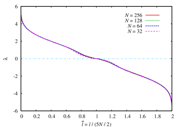
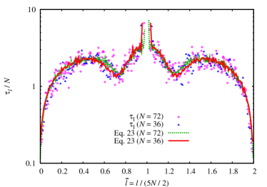
Figure 8: (Color online) Top: Full Lyapunov spectra of rough hard disk systems for various system sizes $N$, plotted as a function of the normalized exponent $\bar{l}=l/(5N/2)$. All systems have a density $\rho=0.7$, and $\kappa=0.4$. The spectra quickly converge to a smooth limit spectrum for $N\to\infty$. Bottom: Lyapunov vector convergence times, divided by $N$, for two system sizes, $N=36$ and $N=72$ as indicated by the keys. The points are direct simulation results, the smooth lines were computed from the Lyapunov spectrum via Eq. (23), where $A=2.85$.

It has been argued in Ref. DHP_2002 that for $\kappa=0$ the decay time for the correlation function $\chi_{1}(t)$ concerning the maximum exponent is determined by $1/(\lambda_{1}-\lambda_{2})$ and, hence, by the inverse ”slope” of the spectrum at $l=1$. These arguments also apply to all the other exponents such that one expects

$$\tau_{l}=\frac{A}{|\lambda_{l+1}-\lambda_{l}|}$$ (23)

to hold, where $A$ is a fitting parameter which, for the choice $\Theta=0.9$, becomes 2.85. Rewriting this expression in terms of the reduced index $\bar{l}=l/(5N/2)$ gives

$$\tau_{l}=\frac{A}{\left|\Delta\lambda(\bar{l})/\Delta\bar{l}\right|\Delta\bar{l}}\approx\frac{5NA}{2}\left|\frac{d\lambda(\bar{l})}{d\bar{l}}\right|^{-1},$$ (24)

where we have replaced the finite differences by the respective differentials. Since the limiting spectral slope, Eq. (22), is independent of $N$, the convergence time for any $l$ is expected to be proportional to the particle number $N$.

Our results for $\tau_{l}/N$ are depicted in the lower panel of Figure 8, where experimental results for $N=36$ and $N=72$ rough disks are shown by the points. Both systems have a density $\rho=0.7$, and $\kappa=0.4$. Clearly the points for different $N$ collapse onto a single curve proving the proportionality of $\tau_{l}$ to $N$. If $\tau_{l}$ is computed from the slope of the Lyapunov spectrum according to Eqs. (23) or (24), the smooth lines are obtained. Their agreement with the simulation points supports our assertion in Eq. (23).

The symmetry obviously exhibited by the convergence time, $\tau_{l}=\tau_{D+1-l}$, is surprising in view of the fact that the algorithm treats successive vectors successively: The orientation of the second vector is affected by that of the first, that of the third vector by that of the first and second, and so on.

IV Conclusions

In this paper we investigate rough hard-disk systems, arguably the most simple models of a molecular fluid with translational and rotational degrees of freedom. The rotation of the particles may be viewed as a mechanism to store internal energy, which is returned to the translational degrees of motion with some delay. We compute Lyapunov spectra and study the effect of rotation-translation coupling on the dynamical stability of such systems.

If the moment of inertia $I$ of the disks vanishes, the translational dynamics is completely decoupled from the rotational degrees of freedom and the results for the smooth hard-disk system are reproduced. If $I$ respective the more relevant coupling parameter $\kappa=4I$ is increased, the Lyapunov spectrum changes drastically with the rotation-dominated parts of the spectrum being gradually filled in, until a separation into translation- and rotation-dominated parts becomes meaningless.

The maximum exponent, $\lambda_{1}$, which is taken as an indicator for dynamical chaos, increases with increasing $\kappa$ for large enough densities ($\rho>0.7$), but decreases for smaller densities. At the same time, the Kolmogorov-Sinai entropy $h_{KS}$ always decreases. The latter, which is the sum of all positive exponents, gives the rate of mixing in phase space, which becomes less and less effective the more important the rotation is for the dynamics. We encounter the unexpected situation that for large densities dynamical chaos may increases with $\kappa$ whereas at the same time phase-space mixing takes longer. This should be contrasted to the behavior of a system of hard dumbbells MP_2002 . For a uniform mass distribution of the dumbbells (corresponding to $\kappa=0.5$ for the rough disks), both $\lambda_{1}$ and $h_{KS}$ increase with the molecular anisotropy, and the mixing time decreases. From this point of view, the rough disk model seems artificial.

Another surprise is the seeming lack of Lyapunov modes for the rough disks with non-vanishing $\kappa$, given the fact that modes were readily found for hard-dumbbell systems MP_2002 . As for soft interaction potential systems, Fourier transformation methods may still give evidence for modes. This point deserves further investigation. However, the localization in physical space of the perturbation vectors associated with the maximum exponent is as expected.

The localization spectrum shown in the bottom panel of Fig. 7 is an application of a projection of the tangent vectors onto the phase space of individual disks. Due to the time-reversal symmetry of the evolution equations, such projections should show definite symmetries with respect to the positive and negative (not included in Fig. 7) branches of the Lyapunov spectrum. However, more often than not, these symmetries are numerically not recovered by the classical algorithm. The explanation lies in the fact that Gram-Schmidt-orthonormalized tangent vectors span the proper subspaces for the computation of the exponents, but are not covariant with the tangent flow Ginelli . If covariant vectors are used, these spurious asymmetries disappear BP_2009 .

Up to now little is known about the mechanism governing the convergence of tangent vectors towards their proper directions. For the rough hard disk systems it is shown that the convergence time for all $l$ vary linearly with the system size, $N$. Furthermore, they are related to the slope of the spectrum at a particular $l$. This view is suggested by the existence of the thermodynamic limit of the specrum.

V Acknowledgments

We thank Hadrien Bosetti for fruitful remarks, and Christoph Dellago and William G. Hoover for interesting discussions. We gratefully acknowledge support from the Austrian Science Foundation (FWF) under grant No. P18798-N20.

References

- (1) H. A. Posch and W. G. Hoover, Phys. Rev. A 38, 473 (1988).
- (2) P. Gaspard, Chaos, Scattering, and Statistical Mechanics, Cambridge University Press, Cambridge, 1998.
- (3) The Weeks-Chandler-Anderson potential contains only the repulslve part of the Lennard-Jones potential and is a good reference potential for perturbation theories of fluids [J.D. Weeks, D. Chandler, and H.C. Anderson, J. Chem. Phys. 54, 5237 (1971)].
- (4) Ja. B. Pesin, Sov. Math. Dokl. 17, 196 (1976).
- (5) Ch. Forster and H. A. Posch, New Journal of Physics 7, 32 (2005).
- (6) S. Toxvaerd, Phys. Rev. Lett. 51, 1971 (1983).
- (7) H.A. Posch, Wm. G. Hoover, and B.L. Holian, Ber. Bunsenges. Phys. Chem. 94, 250 (1990).
- (8) D.M. Heyes and H. Okumura, J. Chem. Phys. 124, 164507 (2006).
- (9) Wm. G. Hoover, Time Reversibility, Computer Simulation and Chaos, World Scientific, Singapore, 1999.
- (10) D. Szasz (ed.) Hard Ball Systems and the Lorenz Gas, Encyclopedia of the mathematical sciences 101, Springer Verlag, Berlin (2000).
- (11) Wm.G. Hoover and H. A. Posch, Chaos 8, 366 (1998).
- (12) Ch. Forster, R. Hirschl, H. A. Posch, and Wm. G. Hoover, Physica D 187, 294 (2004).
- (13) T. Taniguchi and G. P. Morriss, Phys. Rev. E 68, 046203 (2003).
- (14) A. Pikovsky and A. Politi, Nonlinearity 11, 1049 (1998); Phys.Rev. E 63, 036207 (2001).
- (15) Lj. Milanović, H. A. Posch, and Wm. G. Hoover, Molec. Phys. 95, 281 (1998).
- (16) LJ. Milanović and H. A. Posch, J. Molec. Liquids, 96-97, 221 - 244 (2002).
- (17) H. A. Posch and R. Hirschl, “Simulation of Billiards and of Hard-Body Fluids”, in Ref. Szasz , pp. 279 - 314.
- (18) T. Taniguchi and G. P. Morriss, Phys. Rev. E 68, 026218 (2003).
- (19) J.-P- Eckmann, Ch. Forster, H. A. Posch, and E. Zabey, J. Stat. Phys. 118, 813 - 847 (2005).
- (20) H.-L. Yang and G. Radons, Phys. Rev. E 71 036211 (2005); Phys. Rev. Lett. 96, 074101 (2006).
- (21) I. Borzsák, H.A. Posch and A. Baranyai, Phys. Rev. E 53, 3694 (1996).
- (22) O. Kum, Y.H. Shin and E.K. Lee, Phys. Rev. E 58, 7243 (1998).
- (23) G.H. Bryan, Rep. Br. Ass. Advmt. Sci, 83 (1894).
- (24) F.B. Pidduck, Proc. R. Soc. A, 101, 101 (1922).
- (25) S. Chapman and T.G. Cowling, The mathematical theory of non-uniform gases, 3rd. edition, Cambridge University Press, 1990.
- (26) J. O’Dell and B.J. Berne, J. Chem. Phys. 63, 2376 (1975).
- (27) B. J. Berne, J. Chem. Phys. 66, 2821 (1977).
- (28) C.S. Pangali and B.J. Berne, J. Chem. Phys. 67, 4561 (1977).
- (29) J.A. Montgomery, Jr. and B.J. Berne, J. Chem. Phys. 67, 4580 (1977).
- (30) Ch. Dellago, H.A. Posch, and W.G. Hoover, Phys. Rev. E 53, 1485 (1996).
- (31) Ch. Dellago and H.A. Posch, Physica A 240, 68 (1997).
- (32) D.C. Rapaport, The art of molecular dynamics simulation, Cambridge University Press, Cambridge, 1995.
- (33) G. Benettin, L. Galgani, A. Giorgilli, and J.M. Strelcyn, Meccanica 15, 29 (1980).
- (34) I. Shimada and T. Nagashima, Progr. Theor. Phys. (Japan), 61, 1605 (1979).
- (35) F. Scheck, Machanics, Springer Verlag, Berlin, 2005.
- (36) Ch. Dellago and H.A. Posch, Phys. Rev. E 55, R9 (1997).
- (37) N.S. Krylov, Works on the Foundations of Statistical Mechanics (Princeton University Press, Princeton, 1979); Ya. G. Sinai, ibid. p.239.
- (38) G. M. Zaslavsky, Chaos in dynamical Systems (Harwood Academic Publishers, Chur, 1985).
- (39) R. van Zon, H. van Beijeren, and J.R. Dorfman, ”Kinetic theory estimates for the Kolmogorov-Sinai entropy, and the largest Lyapunov exponent for dilute hard ball gases and for dilute random Lorentz gases”, Ref. Szasz , pp. 231 - 278.
- (40) R. van Zon and H. van Beijeren, J. Stat. Phys. 109, Nos. 3/4, 641 (2002).
- (41) Ch. Forster, D. Mukamel, and H.A. Posch, Phys. Rev. E 69, 066124 (2004).
- (42) H. van Beijeren, J.R. Dorfman, H.A. Posch, and Ch. Dellago, Phys. Rev. E 56, 5272 (1997).
- (43) A.S. de Wijn Phys. Rev. E 71, 046211 (2005).
- (44) A.S. de Wijn and H. van Beijeren, Phys. Rev. E 70, 016207 (2004).
- (45) H.A. Posch and Ch. Forster, Lecture Notes on Computational Science – ICCS 2002, ed. P.M.A. Sloot, C.J.K. Tan, J.J.Dongarra, and A.G. Hoekstra, p.1170 (Springer Verlag, Berlin, 2002).
- (46) P. Manneville, Lecture notes in Physics 230, 319 (Springer-Verlag, Berlin, 1985).
- (47) R. Livi and S. Ruffo, Nonlinear Dynamics, ed. G. Turchetti, p. 220, World Scientific, Singapore, 1989.
- (48) M. Falcioni, U.M.B. Marconi, and A. Vulpiani, Phys. Rev. A 44 2263 (1991).
- (49) T. Taniguchi and G.P. Morriss, Phys. Rev. E 73, 036208 (2006).
- (50) G. Jumarie, Relative Information (Springer-Verlag, Berlin, 1990), Sec. 2.11.
- (51) J. van Meel, Lyapunov instability of rough hard-disk fluids, Master’s Thesis (University of Vienna, July 2005).
- (52) H. Bosetti and H.A. Posch, in preparation (2009).
- (53) F. Ginelli, P. Poggi, A. Turchi, H. Chaté, R. Livi, and A. Politi, Phys. Rev. Lett. 99, 130601 (2007).
- (54) Ch. Dellago, Wm. G. Hoover, and H.A. Posch, Phys. Rev. E 65, 056216 (2002).