Three-band s$\pm$ Eliashberg theory and the superconducting gaps of iron pnictides

Abstract

The experimental critical temperatures and gap values of the superconducting pnictides of both the 1111 and 122 families can be simultaneously reproduced within the Eliashberg theory by using a three-band model where the dominant role is played by interband interactions and the order parameter undergoes a sign reversal between hole and electron bands ($s\pm$-wave symmetry). High values of the electron-boson coupling constants and small typical boson energies (in agreement with experiments) are necessary to obtain the values of all the gaps and to correctly reproduce their temperature dependence.

The recently discovered Fe-based pnictide superconductors Kamihara_La ; Ren_Sm ; Rotter_122 have aroused great interest in the scientific community. They have indeed shown that high T_c superconductivity does not uniquely belong to cuprates but can take place in Cu-free systems as well. Nevertheless, as in cuprates, superconductivity occurs upon charge doping of a magnetic parent compound above a certain critical value. However, important differences exist: the parent compound in cuprates is a Mott insulator with localized charge carriers and a strong Coulomb repulsion between electrons; in the pnictides, on the other hand, it is a bad metal and shows a tetragonal to orthorhombic structural transition below $\approx$ 140 K, followed by an antiferromagnetic (AF) spin-density-wave (SDW) order de la Cruz . Charge doping gives rise to superconductivity and, at the same time, inhibits the occurrence of both the static magnetic order and the structural transition. The Fermi surface consists of two or three hole-like sheets around $\Gamma$ and two electron-like sheets around $M$. Up to now, the most intensively studied systems are the 1111 compounds, ReFeAsO_1-xF_x (Re = La, Sm, Nd, Pr, etc.) and especially the 122 ones, hole- or electron-doped AFe₂As₂ (A = Ba, Sr, Ca). The huge amount of experimental work already done in 122 compounds is due to the availability of rather big high-quality single crystals.

Most of the present research effort is spent clarifying the microscopic pairing mechanism responsible for superconductivity. The conventional phonon-mediated coupling mechanism cannot explain the observed high T_c within standard Migdal-Eliashberg theory and the inclusion of multiband effects increases T_c only marginally Boeri_PhysC_SI . On the other hand, the magnetic nature of the parent compound seems to favor a magnetic origin of superconductivity and a coupling mechanism based on nesting-related AF spin fluctuations has been proposed Mazin_spm . It predicts an interband sign reversal of the order parameter between different sheets of the Fermi surface ($s\pm$ symmetry). The number, amplitude and symmetry of the superconducting energy gaps are indeed fundamental physical quantities that any microscopic model of superconductivity has to account for. Experiments with powerful techniques such as ARPES, point-contact spectroscopy, STM etc., have been carried out to study the superconducting gaps in pnictides (for a review see PhysC_Fe ). Although results are sometimes in disagreement with each other, a multi-gap scenario is emerging with evidence for rather high gap ratios, $\Delta_{1}/\Delta_{2}\approx 2-3$ PhysC_Fe . A two-band BCS model cannot account either for the amplitude of the experimental gaps and for their ratio. Three-band BCS models have been investigated Mazin_PhysC_SI ; Benfatto ; Kuchinskii which can reproduce the experimental gap ratio but not the exact experimental gap values. In this regard a reliable study has to be carried out within the framework of the Eliashberg theory for strong coupling superconductors Eliashberg , due to the possible high values of the coupling constants necessary to explain the experimental data.

By using this strong-coupling approach, we show here that the superconducting iron pnictides represent a case of dominant negative interband-channel superconductivity ($s\pm$-wave symmetry) with high values of the electron-boson coupling constants and small typical boson energies. Furthermore we prove that a small contribution of intraband coupling does not affect significantly the obtained results. The model is compared with the results of two representative experiments in 122 Ding_ARPES_BaKFeAs and 1111 Daghero_Sm compounds proving to be able to reproduce fairly well the values and the whole temperature dependence of the superconducting energy gaps.

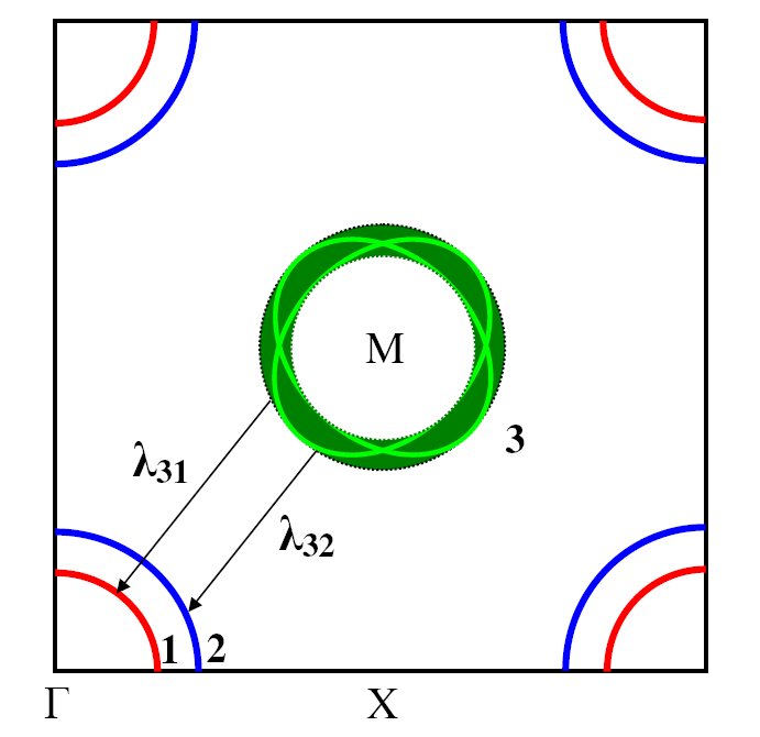
Figure 1: Schematic drawing of the multiband model used in this work. The two hole bands (1 and 2) are centered around the $\Gamma$ point, while the equivalent electron band (3) around the $M$ point of the reduced Brillouin zone.

As a starting point we can model the electronic structure of pnictides by using a three-band model (Fig.1) with two hole bands (1 and 2) and one equivalent electron band (3) Mazin_PhysC_SI . The $s$-wave order parameters of the hole bands have opposite sign with respect to that of the electron one Mazin_spm . Intraband coupling could be provided by phonons while interband coupling by antiferromagnetic spin fluctuations. In a one-band system spin fluctuations (SF) are always pair breaking but in a multiband one the interband term can contribute to increase the critical temperature. Indeed, in the multiband Eliashberg equations (EE) the SF term in the intraband channel has positive sign for the renormalization functions $Z_{i}$ and negative sign for the superconducting order parameters $\Delta_{i}$ thus leading to a strong reduction of T_c. However, if we consider negative interband contributions in the $\Delta_{i}$ equations, the final result can be an increase of the critical temperature Ummaimp .

Let us consider the generalization of the Eliashberg theory Eliashberg for multiband systems, that has already been used with success to study the MgB₂ superconductor Carbinicol . To obtain the gaps and the critical temperature within the s-wave, three-band Eliashberg equations one has to solve six coupled integral equations for the gaps $\Delta_{i}(i\omega_{n})$ and the renormalization functions $Z_{i}(i\omega_{n})$, where $i$ is a band index that ranges between $1$ and $3$ (see Fig.1) and $\omega_{n}$ are the Matsubara frequencies. For completeness we included in the equations the non-magnetic and magnetic impurity scattering rates in the Born approximation, $\Gamma^{N}_{ij}$ and $\Gamma^{M}_{ij}$:

$$\omega_{n}Z_{i}(i\omega_{n})=\omega_{n}+\sum_{j}(\Gamma^{N}_{ij}+\Gamma^{M}_{ij})N^{Z}_{j}(i\omega_{n})+$$ (1)

$$\pi T\sum_{m,j}\Lambda^{Z}_{ij}(i\omega_{n},i\omega_{m})N^{Z}_{j}(i\omega_{m})$$

$$Z_{i}(i\omega_{n})\Delta_{i}(i\omega_{n})=\sum_{j}(\Gamma^{N}_{ij}-\Gamma^{M}_{ij})N^{\Delta}_{j}(i\omega_{n})+$$ (2)

$$\pi T\sum_{m,j}[\Lambda^{\Delta}_{ij}(i\omega_{n},i\omega_{m})-\mu^{*}_{ij}(\omega_{c})]\theta(\omega_{c}-|\omega_{m}|)N^{\Delta}_{j}(i\omega_{m})$$

where $\Lambda^{Z}_{ij}(i\omega_{n},i\omega_{m})=\Lambda^{ph}_{ij}(i\omega_{n},i\omega_{m})+\Lambda^{sp}_{ij}(i\omega_{n},i\omega_{m})$, $\Lambda^{\Delta}_{ij}(i\omega_{n},i\omega_{m})=\Lambda^{ph}_{ij}(i\omega_{n},i\omega_{m})-\Lambda^{sp}_{ij}(i\omega_{n},i\omega_{m})$. $\theta$ is the Heaviside function and $\omega_{c}$ is a cut-off energy. In particular, $\Lambda^{ph,sp}_{ij}(i\omega_{n},i\omega_{m})=\int_{0}^{+\infty}d\Omega\alpha^{2}_{ij}F^{ph,sp}(\Omega)/[(\omega_{n}-\omega_{m})^{2}+\Omega^{2}]$, where $ph$ means “phonon”  and $sp$ “spin fluctuations”. Finally, $N^{\Delta}_{j}(i\omega_{m})=\Delta_{j}(i\omega_{m})/{\sqrt{\omega^{2}_{m}+\Delta^{2}_{j}(i\omega_{m})}}$ and $N^{Z}_{j}(i\omega_{m})=\omega_{m}/{\sqrt{\omega^{2}_{m}+\Delta^{2}_{j}(i\omega_{m})}}$.

In principle the solution of the three-band EE shown in eqs.1 and 2 requires a huge number of input parameters: i) nine electron-phonon spectral functions, $\alpha^{2}_{ij}F^{ph}(\Omega)$; ii) nine electron-SF spectral functions, $\alpha^{2}_{ij}F^{sp}(\Omega)$; iii) nine elements of the Coulomb pseudopotential matrix, $\mu^{*}_{ij}(\omega_{\rm c})$; iv) nine non-magnetic ($\Gamma^{N}_{ij}$) and nine paramagnetic ($\Gamma^{M}_{ij}$) impurity scattering rates.
It is obvious that a practical solution of these equations requires a drastic reduction in the number of free parameters of the model. On the other hand, from the work of Mazin et al. Mazin_PhysC_SI we know that: i) $\lambda^{ph}_{ii}>>\lambda^{ph}_{ij}\approx 0$ i.e. phonons mainly provide intraband coupling but the total electron-phonon coupling constant $\Sigma_{i}\lambda^{ph}_{ii}$ should be very small Boeri_PhysC_SI , ii) $\lambda^{sp}_{ij}>>\lambda^{sp}_{ii}\approx 0$, i.e. SF mainly provide interband coupling. We include these features in the most simple three-band model by posing: $\lambda^{ph}_{ii}=\lambda^{ph}_{ij}=0$, $\lambda^{sp}_{ii}=0$ and $\mu^{*}_{ii}(\omega_{\rm c})=\mu^{*}_{ij}(\omega_{\rm c})=0$. In addition, we set $\Gamma^{N}_{ij}=\Gamma^{M}_{ij}=0$ in eqs. (1) and (2).

Under these approximations, the electron-boson coupling-constant matrix is then Mazin_PhysC_SI :

$$\left(\begin{array}[]{ccc}0&0&\lambda_{31}\nu_{1}\\ 0&0&\lambda_{32}\nu_{2}\\ \lambda_{31}&\lambda_{32}&0\\ \end{array}\right)$$

where $\nu_{1}=N_{1}(0)/N_{3}(0)$, $\nu_{2}=N_{2}(0)/N_{3}(0)$ and $N_{i}(0)$ is the normal density of states at the Fermi level for the $i$-band ($i=1,2,3$ according to Fig.1).

We initially solved the EE on the imaginary axis to calculate the critical temperature and, by means of the technique of the Padè approximants, to obtain the low-temperature value of the gaps. In presence of a strong coupling interaction or of impurities, however, the value of $\Delta_{i}(i\omega_{n=0})$ obtained by solving the imaginary-axis EE can be very different from the value of $\Delta_{i}$ obtained from the real-axis EE Ummastrong . Therefore, in order to determine the exact temperature dependence of the gaps, we then solved the three-band EE in the real-axis formulation.

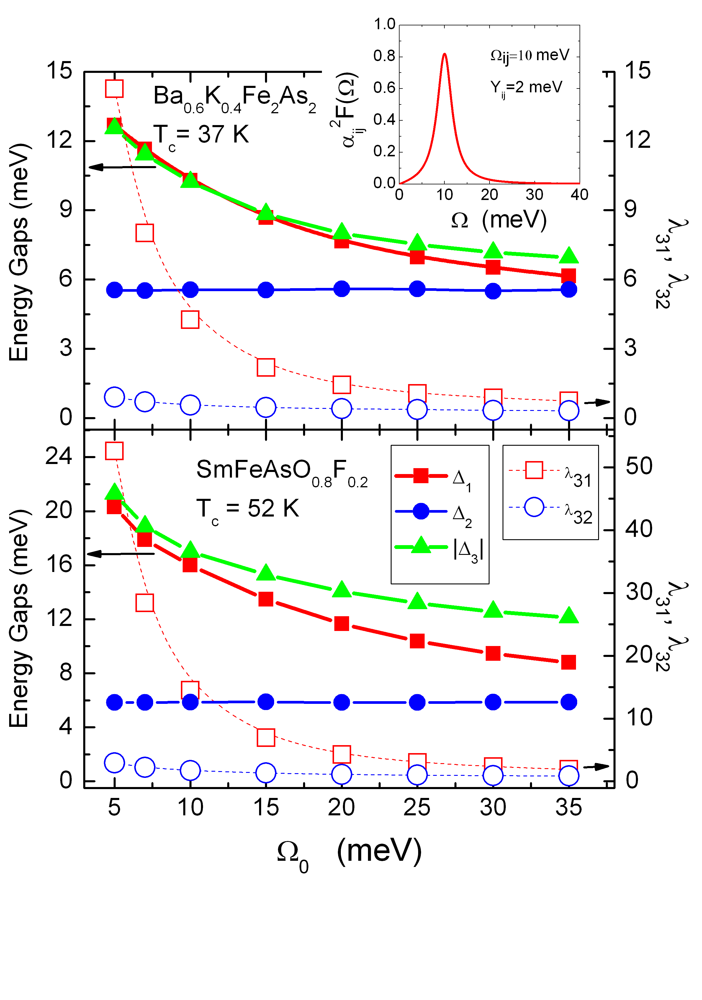
Figure 2: Full symbols, left axis: Calculated gap values at $T$=2 K for Ba_0.6K_0.4Fe₂As₂ (upper panel) and SmFeAsO_0.8F_0.2 (lower panel) as function of typical boson energy $\Omega_{0}$. Open symbols, right axis: Electron-boson coupling constants, $\lambda_{31}$ and $\lambda_{32}$ as function of $\Omega_{0}$. The inset shows the spectral function used in this model in the case $\Omega_{ij}=10$ meV.

We tried to reproduce the critical temperature and the gap values in two representative cases: i) the 122 compound Ba_0.6K_0.4Fe₂As₂ with $T_{c}=37$ K where ARPES measurements gave $\Delta_{1}(0)\approx 12.1$ meV, $\Delta_{2}(0)\approx 5.5$ meV and $\Delta_{3}(0)\approx 12.8$ meV Ding_ARPES_BaKFeAs ; ii) the 1111 compound SmFeAsO_0.8F_0.2 with $T_{c}=52$ K where from point-contact spectroscopy measurements we obtained $\Delta_{1}(0)=18\pm 3$ meV and $\Delta_{2}(0)=6.15\pm 0.45$ meV Daghero_Sm .

Inelastic neutron-scattering experiments suggest that the typical boson energy possibly responsible for superconductivity ranges roughly between 10 and 30 meV neutroni . In our numerical simulations we used spectral functions with Lorentzian shape, i.e. $\alpha^{2}_{ij}F(\Omega)=C_{ij}[L(\Omega+\Omega_{ij},Y_{ij})-L(\Omega-\Omega_{ij},Y_{ij})]$ where $L(\Omega\pm\Omega_{ij},Y_{ij})=[(\Omega\pm\Omega_{ij})^{2}+(Y_{ij})^{2}]^{-1}$, $C_{ij}$ are the normalization constants necessary to obtain the proper values of $\lambda_{ij}$, while $\Omega_{ij}$ and $Y_{ij}$ are the peak energies and half-widths, respectively. In all our calculations we always set $\Omega_{ij}=\Omega_{0}$, with $\Omega_{0}$ ranging between 5 and 35 meV and $Y_{ij}=2$ meV. The cut-off energy is $\omega_{c}=12\cdot\Omega_{0}$ and the maximum quasiparticle energy is $\omega_{max}=16\cdot\Omega_{0}$.

In the 122 case ($T_{c}=37$ K) we know that $\nu_{1}=1$ and $\nu_{2}=2$ Mazin_PhysC_SI while in the 1111 case ($T_{c}=52$ K) we have $\nu_{1}=0.4$ and $\nu_{2}=0.5$ Mazin4 . Once the energy of the boson peak, $\Omega_{0}$ is set, only two free parameters are left in the model: $\lambda_{31}$ and $\lambda_{32}$.

By properly selecting the values of these parameters it is relatively easy to obtain the experimental values of the critical temperature and of the small gap. It is more difficult to reproduce the values of the large gaps of band 1 and 3 since, due to the high $2\Delta_{1,3}/k_{B}T_{c}$ ratio (of the order of 8-9), high values of the coupling constants and small boson energies are required. Fig.2 shows the values of the calculated gaps (full symbols, left axis) as function of the boson peak energy, $\Omega_{0}$. The corresponding values of $\lambda_{31}$ and $\lambda_{32}$, chosen in order to reproduce the values of T_c and of the small gap, $\Delta_{2}$, are also shown in the figure (open symbols, right axis). In both materials, only when $\Omega_{0}\leq 10$ meV the value of the large gaps correspond to the experimental data. Indeed, when $\Omega_{0}$ increases, the values of $\Delta_{1}$ and $\Delta_{3}$ strongly decrease. As a consequence, a rather small energy of the boson peak together with a very strong coupling (particularly in the 3-1 channel) is needed in order to obtain the experimental $T_{c}$ and the correct gap values. In this regard, it is worth noticing that the absolute values of the large gaps cannot be reproduced in a interband-only, two-band Eliashberg model dolghi3 as well as within a three-band BCS model. In the latter case it is only possible to obtain a ratio of the gaps close to the experimental one Kuchinskii ; Benfatto .

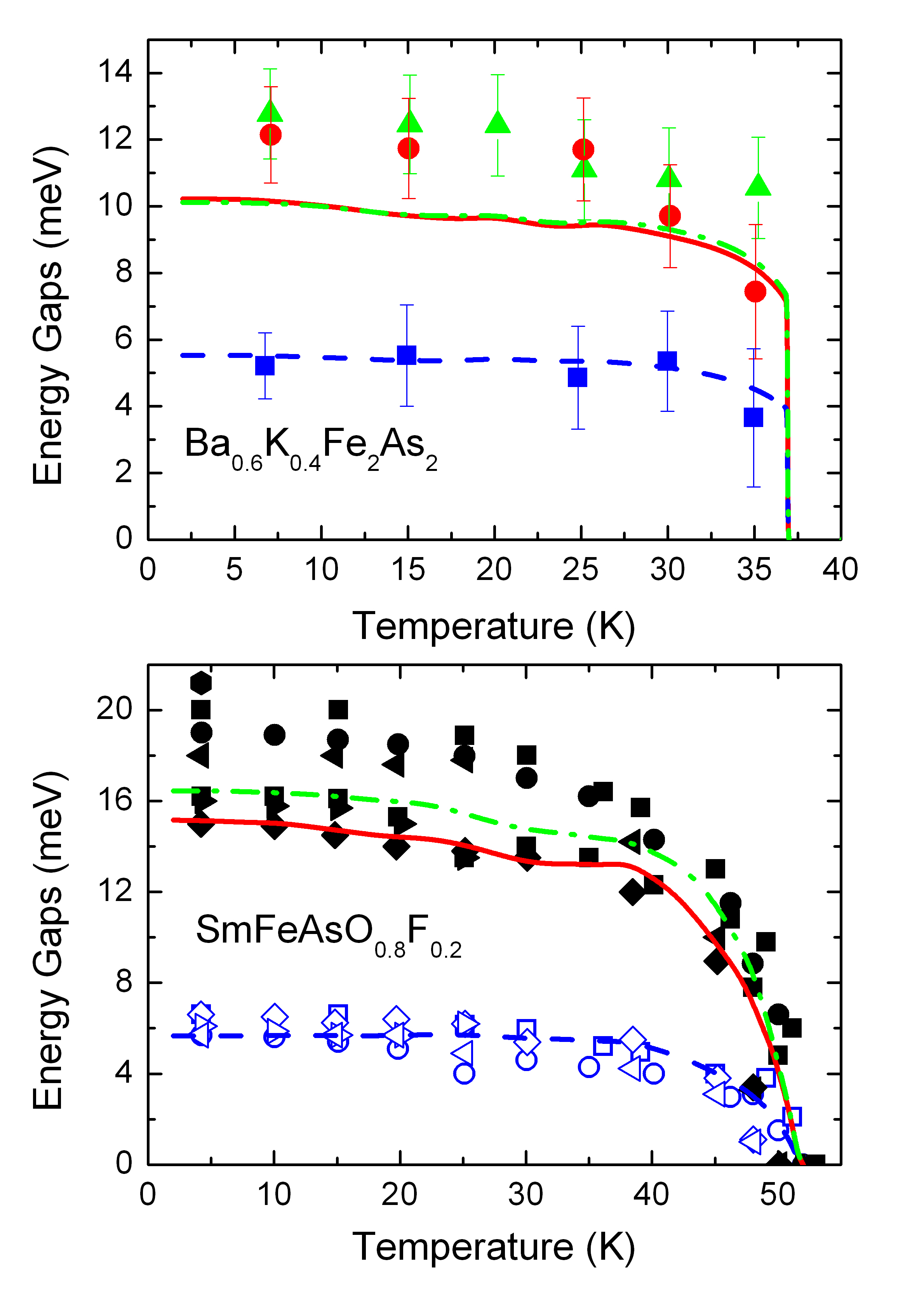
Figure 3: Calculated temperature dependence of the gaps for Ba_0.6K_0.4Fe₂As₂ ($T_{c}=37$ K, upper panel) and for SmFeAsO_0.8F_0.2 ($T_{c}=52$ K, lower panel): $\Delta_{1}(T)$ (red solid line), $\Delta_{2}(T)$ (blue dashed line) and $\Delta_{3}(T)$ (green dash-dot line). Symbols are experimental data from ref. Ding_ARPES_BaKFeAs (upper panel) and ref. Daghero_Sm (lower panel).

$\lambda_{31}=3.866$	$\lambda_{32}=0.471$	$\mu^{*}_{ij}=0$, $\lambda_{ii}=0.4$
$\Delta_{1}=10.30$ meV	$\Delta_{2}=5.62$ meV	$|\Delta_{3}|=10.24$ meV

Table 1: The effect of a small contribution of intraband coupling, $\lambda_{ii}=0.4$ for the case of Ba_0.6K_0.4Fe₂As₂ at $T=2$ K.

Another important result of the model is the temperature dependence of the gaps. Figure 3 shows this dependence for the experimental gaps (symbols) together with the theoretical $\Delta_{i}(T)$ curves obtained by the three-band Eliashberg model (lines) for Ba_0.6K_0.4Fe₂As₂ (upper panel) and SmFeAsO_0.8F_0.2 (lower panel). The parameters used for the 122 compound are $\Omega_{0}=10$ meV, $\lambda_{31}=4.267$ and $\lambda_{32}=0.569$; for the 1111 compound we used $\Omega_{0}=10$ mev, $\lambda_{31}=14.520$ and $\lambda_{32}=1.708$. The experimental temperature dependence of the gaps shown in the upper panel is rather unusual with the gaps slightly decreasing with increasing temperature until they suddenly drop close to $T_{c}$. The theory reproduces very well this behavior, which is possible only in a very strong coupling regime Ummastrong . The different temperature dependence observed in the lower panel of Fig. 3 results from a complex non-linear dependence of $\Delta_{i}$ vs. $T$ curves on $\lambda_{31}$. Further details will be given in a forthcoming paper.

We also tested the effect into the model of a small intraband coupling (possibly of phonon origin). In the case of Ba_0.6K_0.4Fe₂As₂ we used $\lambda_{ii}=0.4$ since we know indeed that this coupling cannot be very high Boeri_PhysC_SI . It might be thought that this term can sensibly contribute to increase the gap values but, as can be seen in Table 1, this is not the case: the gap values only show a slight increase (of the order of 1%).

$\lambda_{31}=2.730$	$\lambda_{32}=0.758$	$\mu^{*}_{ij}=0.1$, $\lambda_{ii}=0.4$
$\Delta_{1}=7.49$ meV	$\Delta_{2}=5.72$ meV	$|\Delta_{3}|=7.98$ meV

Table 2: The effect of the Coulomb interaction, $\mu^{*}_{ij}$ for the case shown in Table 1.

The effect of Coulomb interaction was also investigated for the case shown in Table 1 where a weak intraband coupling is included. We chose $\mu^{*}_{ij}=0.1$ and, as expected, we found that the intraband Coulomb pseudopotential has a negligible effect while the interband one Ummaimp strongly contributes to raise $T_{c}$ and reduces in a considerable way the value of $\lambda_{31}$: in this case, as shown in Table 2, it is only possible to obtain the correct value of the small gap. As a consequence, this result seems to exclude a strong interband Coulomb interaction in these compounds.

Finally we have also examined, for SmFeAsO_0.8F_0.2, the case of a spectral function with two peaks at energies $\Omega_{1}$ and $\Omega_{2}$. In the upper panel of Fig. 4 the two boson energies are $\Omega_{1}=10$ meV and $\Omega_{2}=20$ meV, while in the lower panel we have $\Omega_{1}=10$ meV and $\Omega_{2}=30$ meV. The gap values (left axis) and the coupling constants, $\lambda_{31}$ and $\lambda_{32}$ (right axis) are plotted as a function of the weight of the low-energy peak, w_p. As somehow expected, when the weight of this peak is larger, (w_p = 0.75) the gaps $\Delta_{1}$ and $\Delta_{3}$ are larger and close to the experimental ones but the coupling constants, $\lambda_{31}$ and $\lambda_{32}$ strongly increase.

In conclusion, we have shown that the newly discovered iron pnictides very likely represent a case of dominant negative interband-channel pairing superconductivity where an electron-boson coupling, such as the electron-SF one, can became a fundamental ingredient to increase $T_{c}$ in a multiband strong-coupling picture. In particular, the present results prove that a simple three-band model in strong-coupling regime can reproduce in a quantitative way the experimental $T_{c}$ and the energy gaps of the pnictide superconductors with only two free parameters, $\lambda_{31}$ and $\lambda_{32}$, provided that the typical energies of the spectral functions are of the order of 10 meV and the coupling constants are very high ($\lambda_{31}>4$).

We thank I.I. Mazin and E. Cappelluti for useful discussions.

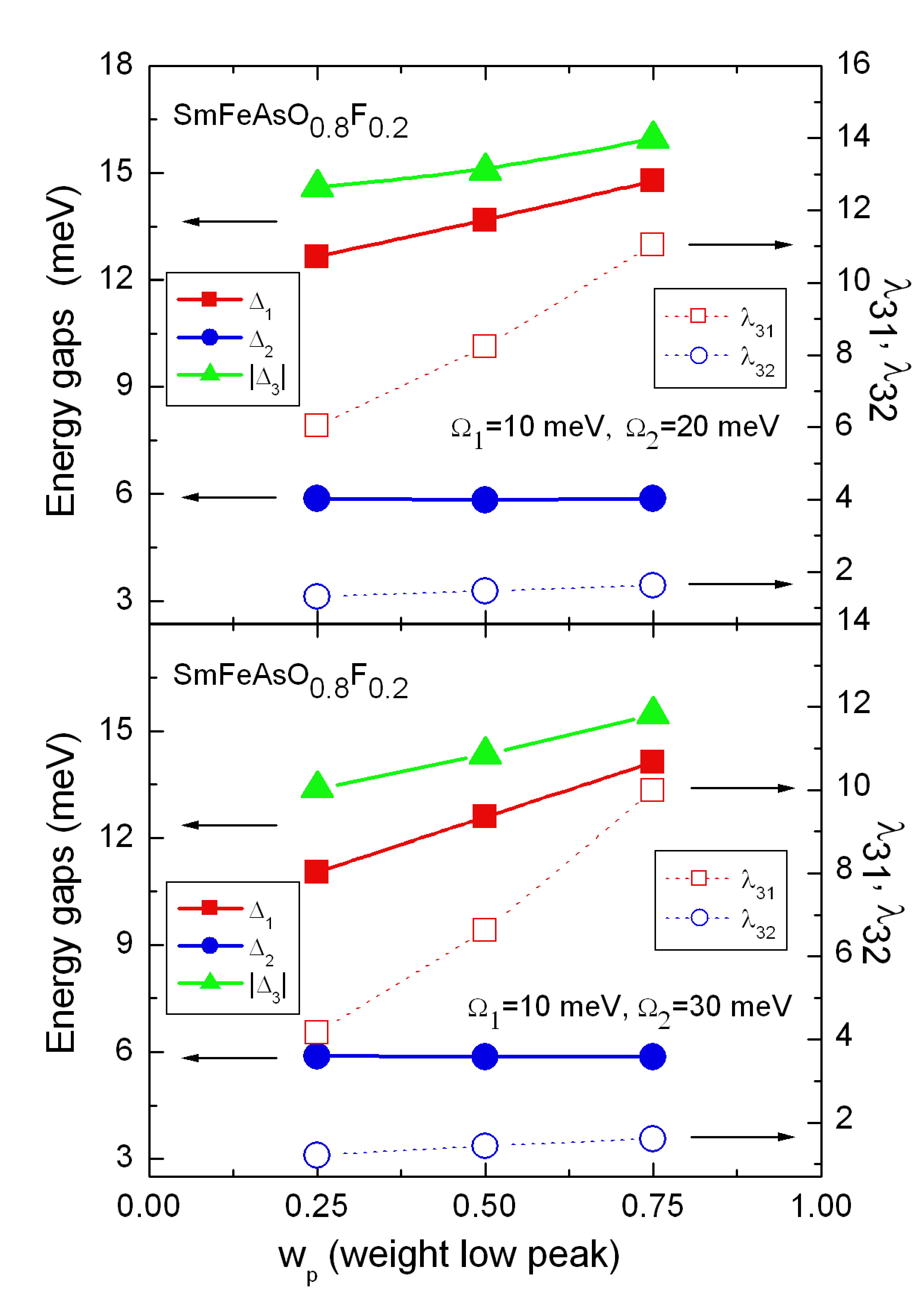
Figure 4: The calculated gaps and electron-boson coupling constants $\lambda_{31}$ and $\lambda_{32}$ in the 1111 case as function of the weight $w_{p}$ of the low-energy peak $\Omega_{1}$. $\Omega_{2}=20$ meV (upper panel) and 30 meV (lower panel).

References

- (1) Y. Kamihara, et al., J. Am. Chem. Soc. 130, 3296-3297 (2008).
- (2) Z.A. Ren, et al., Chin. Phys. Lett. 25, 2215 (2008).
- (3) M.Rotter, et al., Phys.Rev.Lett. 101, 107006 (2008).
- (4) Clarina de la Cruz, et al., Nature, 453, 899 (2008).
- (5) L. Boeri, O.V. Dolgov and A.A. Golubov, Phys. Rev. Lett. 101, 026403 (2008); L. Boeri et al., to appear in Physica C Special Issue on Pnictides, arXiv:0902.0288 (2009).
- (6) I.I. Mazin et al., Phys. Rev. Lett. 101, 057003 (2008).
- (7) Physica C, Special Issue on Pnictides (2009), in press.
- (8) I.I. Mazin and J. Schmalian, to appear in Physica C Special Issue on Pnictides, arXiv:0901.4790 (2009).
- (9) L. Benfatto et al., Phys. Rev. B 78, 140502(R) (2008).
- (10) E.Z. Kuchinskii and M.V. Sadovskii, arXiv:0901.0164 (2009).
- (11) G.M. Eliashberg, Sov. Phys. JETP 3, 696 (1963).
- (12) H. Ding et al., Europhys. Lett., 83, 47001 (2008).
- (13) D. Daghero et al., arXiv:0812.1141v1 (2008); R.S. Gonnelli et al., to appear in Physica C Special Issue on Pnictides, arXiv:0902.3441 (2009).
- (14) G.A. Ummarino, J. Supercond. Nov. Magn. 20, 639 (2007).
- (15) E.J. Nicol, J.P. Carbotte, Phys. Rev. B 71, 054501 (2005); G.A.Ummarino, et al., Physica C 407, 121 (2004).
- (16) G.A.Ummarino and R.S. Gonnelli, Physica C 328, 189 (1999).
- (17) A. D. Christianson et al., Nature 456, 930 (2008); R. Osborn, et al., to appear in Physica C Special Issue on Pnictides, arXiv:0902.3760, (2009).
- (18) I.I. Mazin, private communication.
- (19) O.V. Dolgov, et al., Phys. Rev. B 79, 060502(R) (2009); G.A. Ummarino, to be published in J. Supercond. Nov. Magn.