Liquid Nanofilms.
A Mechanical Model for the Disjoining Pressure

Abstract

Liquids in contact with solids are submitted to intermolecular forces making liquids heterogeneous and, in a mechanical model, the stress tensor is not any more spherical as in homogeneous bulks. The aim of this article is to show that a square-gradient functional taking into account the volume liquid free energy corrected with two surface liquid density functionals is a mean field approximation allowing to study structures of very thin liquid nanofilms near plane solid walls. The model determines analytically the concept of disjoining pressure for liquid films of thicknesses of a very few number of nanometers and yields a behavior in good agreement with the shapes of experimental curves carried out by Derjaguin and his successors.

1 Introduction

The technical development of sciences allows us to observe phenomena at length scales of a very few number of nanometers. This nanomechanics infers applications in numerous fields, including medicine and biology. It reveals new behaviors, often surprising and essentially different from those that are usually observed at macroscopic and also at microscopic scales [1]. Currently simple models proposing realistic qualitative behaviors need to be developed in different fields of nanosciences even if their comparison with experimental data may be criticized at a quantitative level.
As pointed out in experiments with water, the density of liquid water is found to be changed in narrow pores [2]. The first reliable evidence of this effect was reported by V.V. Karasev, B.V. Derjaguin and E.N. Efremova in 1962 and found after by many others ([3], pages 240-244). In order to evaluate the structure of thin interlayers of water and other liquids, Green-Kelly and Derjaguin employed a method based on measuring changes in birefringence [4]; they found significant anisotropy of water interlayers.
In a recent article, the equations of motion of thin films were considered by taking into account the variation of the disjoining pressure along the layer [5]. The aim of this paper is to study, by means of a continuous mechanical model, the disjoining pressure and the behavior for very thin liquid films at the mesoscopic scale of a few number of nanometers.

Since van der Waals at the end of the nineteenth century, the fluid inhomogeneities in liquid-vapor interfaces were represented in continuous models by taking into account a volume energy depending on space density derivative [6, 7, 8, 9, 10]. Nevertheless, the corresponding square-gradient functional is unable to model repulsive force contributions and misses the dominant damped oscillatory packing structure of liquid interlayers near a substrate wall [11, 12]. Furthermore, the decay lengths are correct only close to the liquid-vapor critical point where the damped oscillatory structure is subdominant [13]. In mean field theory, weighted density-functional has been used to explicitly demonstrate the dominance of this structural contribution in van der Waals thin films and to take into account long-wavelength capillary-wave fluctuations as in papers that renormalize the square-gradient functional to include capillary wave fluctuations [14]. In contrast, fluctuations strongly damp oscillatory structure and it is mainly for this reason that van der Waals’ original prediction of a hyperbolic tangent is so close to simulations and experiments [15].
To propose an analytic expression in density-functional theory for liquid film of a very few nanometer thickness near a solid wall, we add a liquid density-functional at the solid surface and a surface density functional at the liquid-vapor interface to the square-gradient functional representing the volume free energy of the fluid. This kind of functional is well-known in the literature [16]. It was used by Cahn in a phenomenological form, in a well-known paper studying wetting near a critical point [17]. An asymptotic expression is obtained in [18] with an approximation of hard sphere molecules and London potentials for liquid-liquid and solid-liquid interactions: in this way, we took into account the power-law behavior which is dominant in a thin liquid film in contact with a solid.
The disjoining pressure $\Pi$ is a well adapted tool for a very thin liquid film of thickness $h$. In cases of Lifshitz analysis [19] and van der Waals theory, the disjoining pressure behaviors are respectively as $\Pi\sim h^{-3}$ and $\Pi\sim\exp(-h)$. None of them represents correctly experimental results for a film with a thickness ranging over a few nanometers.
Then, the gradient expansion missing the physically dominant damped oscillatory packing structure of the liquid near a substrate wall and only working up a smooth exponential decay is corrected by surface energies issued from London forces which model power-law dispersion interaction: since the only structure that the square gradient functional can yield is monotonic exponential, the surface energies take account of the eventual dominance of attractive power-law dispersion interactions. In fact power-law wings are physically present for liquid film of several nanometers and it is the reason we propose a study only for films in a range of few nanometers.

2 The density-functional

In our model, the free energy density-functional of an inhomogeneous liquid in a domain $O$ of boundary $\partial O$ is taken in the general form

$$F=\int\int\int_{O}\varepsilon\ dv+\int\int_{\partial O}\varphi\ ds,$$ (1)

where $\varepsilon$ is the specific free energy and $\varphi$ is a generic surface free energy of $\partial O$.
In our problem, we consider a horizontal plane liquid layer $(L)$ contiguous to its vapor bulk and in contact with a plane solid wall $(S)$; the z-axis is perpendicular to the solid surface $(S)$. The liquid film thickness is denoted by $h$. Far from its critical point, the liquid at level $z=h$ is situated at a distance order of two molecular diameters from the vapor bulk and the liquid-vapor interface is assimilated to a surface $(\Sigma)$ at $z=h$. Then, the free energy density-functional (1) gets the particular form

$$F=\int\int\int_{(L)}\varepsilon\ dv+\int\int_{(S)}\phi\ ds+\int\int_{(\Sigma)}\psi\ ds.$$ (2)

where $\varphi$ is shared in two parts $\phi$ and $\psi$ respectively associated with $(S)$ and $(\Sigma)$.

$\bullet\quad$ In Rel. (2), the first integral (energy of volume $(L)$) is associated with square-gradient approximation when we introduce a specific free energy of the fluid

$$\varepsilon=\varepsilon(\rho,\beta)$$

at a given temperature $\theta$ as a function of density $\rho$ and $\beta=(\mathrm{grad\,\rho)^{2}}$. Specific free energy $\varepsilon$ characterizes both fluid properties of compressibility and molecular capillarity of liquid-vapor interfaces. In accordance with gas kinetic theory [20], scalar $\lambda=2\rho\,\varepsilon_{,\beta}(\rho,\beta)$ (where $\varepsilon_{,\beta}$ denotes the partial derivative with respect to $\beta$) is assumed to be constant at a given temperature and

$$\rho\,\varepsilon=\rho\,\alpha(\rho)+\frac{\lambda}{2}\,(\text{grad\ }\rho)^{2},$$ (3)

where the term $({\lambda}/{2})\,(\mathrm{grad\ \rho)^{2}}$ is added to the volume free energy $\rho\,\alpha(\rho)$ of a compressible homogeneous fluid. We denote the pressure term associated with specific free energy $\alpha(\rho)$ by

$$P(\rho)=\rho^{2}\alpha^{\,\prime}(\rho).$$ (4)

$\bullet\quad$ In Rel. (2), the second integral (energy of surface $(\Sigma)$) is defined through a model of molecular interactions between the fluid and the solid wall. In fact, near a solid wall, the London potentials of liquid-liquid and liquid-solid interactions are

$$\left\{\begin{array}[]{c}\displaystyle\;\;\;\;\;\;\varphi_{ll}=-\frac{c_{ll}}{r^{6}}\;,\text{ \ when\ }r>\sigma_{l}\;\;\text{and }\;\ \varphi_{ll}=\infty\text{ \ when \ }r\leq\sigma_{l}\,,\\ \displaystyle\;\;\;\;\;\;\varphi_{ls}=-\frac{c_{ls}}{r^{6}}\;,\text{ \ when\ }r>\delta\;\;\text{and }\;\ \varphi_{ls}=\infty\text{ \ when \ }r\leq\delta\;,\end{array}\right.$$

where $c_{ll}$ and $c_{ls}$ are two positive constants, $\sigma_{l}$ and $\sigma_{s}$ denote liquid (fluid) and solid molecular diameters, $\delta=\frac{1}{2}(\sigma_{l}+\sigma_{s})$ is the minimal distance between centers of liquid and solid molecules [21]. In the theory of additive and non-retarded molecular interactions, coefficients $c_{ll}$ and $c_{ls}$ are connected with Hamaker constants $A_{ll}$ and $A_{ls}$ through the relations $A_{ll}=\pi^{2}c_{ll}\rho_{l}^{2}$ and $A_{ls}=\pi^{2}c_{ls}\rho_{l}\rho_{s}$, where $\rho_{l}$ and $\rho_{s}$ respectively denote liquid bulk and solid densities [22]. Forces between liquid and solid have short range and can be simply described by adding a special energy at the surface. This is not the entire interfacial energy: another contribution comes from the distortions in the liquid density profile near the wall [18, 23]. Finally, for a plane solid wall (at a molecular scale), this surface free energy is obtained in the form

$$\phi(\rho)=-\gamma_{1}\rho+\frac{1}{2}\,\gamma_{2}\,\rho^{2}.$$ (5)

Here $\rho$ denotes the liquid density value at the wall. The constants $\gamma_{1}$, $\gamma_{2}$ are positive and given by the relations $\displaystyle\gamma_{1}=\frac{\pi c_{ls}}{12\delta^{2}m_{l}m_{s}}\rho_{s}$, $\displaystyle\gamma_{2}=\frac{\pi c_{ll}}{12\delta^{2}m_{l}^{2}}$ , where $m_{l}$ et $m_{s}$ respectively denote the masses of liquid (fluid) and solid molecules [18]. Moreover, we have $\displaystyle\lambda=\frac{2\pi c_{ll}}{3\sigma_{l}\,m_{l}^{2}}$ .
$\bullet\quad$ In Rel. (2), let us consider the third integral. The conditions in the vapor bulk are $\displaystyle\mathrm{grad}\,\rho=0$ and $\Delta\rho=0$ with $\Delta$ denoting the Laplace operator. Far from the critical point, a way to compute the total free energy of the complete liquid-vapor layer is to add the energy of the liquid layer $(L)$ located between $z=0$ and $z=h$ (first integral of Rel. (2)), the surface energy of the solid wall $(S)$ at $z=0$ (second integral of Rel. (2)), the energy of the liquid-vapor interface of a few Angström thickness assimilated to a surface $(\Sigma)$ at $z=h$ and the energy of the vapor layer located between $z=h$ and $z=+\infty$ [24]. The liquid at level $z=h$ is situated at a distance order of two molecular diameters from the vapor bulk and the vapor has a negligible density with respect to the liquid density [25]. In our model, these two last energies can be expressed by writing a unique energy $\psi$ per unit surface located on the mathematical surface $(\Sigma)$ at $z=h$ : by a calculation like in [18], we can write $\psi$ in a form analogous to expression (5) and also expressed in [23] in the form $\psi(\rho)=-\gamma_{5}\rho+\frac{1}{2}\,\gamma_{4}\,\rho^{2}$; but with a wall corresponding to a negligible density, $\gamma_{5}\simeq 0$ and the surface free energy $\psi$ is reduced to

$$\psi(\rho)=\frac{\gamma_{4}}{2}\ \rho^{2},$$ (6)

where $\rho$ is the liquid density at level $z=h$ and $\gamma_{4}$ is associated with a distance of the order of the fluid molecular diameter (when $\sigma_{l}\simeq\delta$, then $\gamma_{4}\simeq\gamma_{2}$). Consequently, due to the small vapor density, the surface free energy $\psi$ is the same as the one of a liquid in contact with a vacuum and expressed by the third integral of Rel. (2).

Such a form of density functional restricted to the first two integrals was primary expressed by Cahn; Cahn’s study used a graphic representation where energy integrals were presented as different areas in an energy-density plane [17]. Analytical computations were also tested in [24] but without taking account of a complete volume free energy in form (3).
With our previous functional approximation, we obtain the equations of equilibrium (or motion) and boundary conditions for a thin liquid film damping a solid wall. We can compute the liquid layer thickness. The normal stress vector acting on the wall remains constant through the layer and corresponds to the gas-vapor bulk pressure which is usually the atmospheric pressure.
We obtain analytical results expressing the profile of density of very thin layer at a mesoscopic scale. We deduce an analytic expression of the disjoining pressure computed for different solid materials in contact with nanometer scale liquid layers. For all I know, such results have not been obtained in the literature by using both a continuous mechanical model and a differential equation system.
It is wondering to observe that the density-functional theory expressed by a simple model correcting van der Waals’ one with surface density-functionals at the wall and the interface, enables to obtain a representation of the disjoining pressure for very thin films which fits in with experiments by Derjaguin and others. This result is obtained without too complex weighted density-functionals and without taking account of quantum effects corresponding to an Angström length scale. So, this kind of functional may be a good tool to analytically study liquids in contact with solids at a very small nanoscale range.

3 Equation of motion and boundary conditions

In case of equilibrium, functional $F$ is minimal with respect to the vector fields of virtual displacement classically defined (as in [26]) and yields the equation of equilibrium of the inhomogeneous liquid and the boundary conditions between liquid, vapor and solid wall. In case of motions we simply add the inertial forces and the dissipative stresses in the equation of equilibrium (to refer to the well-known explicit calculations, see for example [5, 27, 28]).

3.1 Equation of motion

The equation of motion is

$$\rho\ \mathbf{\Gamma}=\text{div}\left(\mathbf{\sigma}+\mathbf{\sigma}_{v}\right)-\rho\;\text{grad }\Omega,$$ (7)

where $\mathbf{\Gamma}$ is the acceleration vector, $\Omega$ the body force potential, $\mathbf{\sigma}$ the stress tensor generalization and $\mathbf{\ \sigma}_{v}$ the viscous stress tensor,

$$\mathbf{\ \sigma=}-p\,\mathbf{1}-\lambda\;\text{grad\ }\rho\ \otimes\ \text{grad }\rho,$$

where $p=\rho^{2}\varepsilon_{,\rho}-\rho\text{ div{\ }}(\lambda\text{ grad }\rho)$ is different from the pressure term $P$ defined in (4).
For a horizontal layer, in an orthogonal system of coordinates such that the third coordinate $z$ is the vertical direction, all physical quantities in the layer depend only on $z$ and the stress tensor $\mathbf{\sigma}$ of the thin film gets the form

$$\mathbf{\sigma}=\left[\begin{array}[]{ccc}a_{1}&0&0\\ 0&a_{2}&0\\ 0&0&a_{3}\end{array}\right],\quad\mathrm{with}\quad\left\{\begin{array}[]{lll}a_{1}&=&a_{2}=-p,\quad\displaystyle p=P(\rho)-\frac{\lambda}{2}\left(\frac{d\rho}{dz}\right)^{2}-\lambda\,\rho\,\frac{d^{2}\rho}{dz^{2}}\,,\\ a_{3}&=&\displaystyle{-p-\lambda\left(\frac{d\rho}{dz}\right)^{2}.}\end{array}\right.$$

Let us consider a thin film of liquid at equilibrium (gravity forces are neglected). The equation of equilibrium is

$$\text{div }\mathbf{\sigma=0}\,.$$ (8)

Equation (8) yields a constant value for the eigenvalue $a_{3}$,

$$p+{\lambda}\left(\frac{d\rho}{dz}\right)^{2}=P_{v_{b}}\text{,}$$

or

$$P+\,\frac{\lambda}{2}\left(\frac{d\rho}{dz}\right)^{2}-\,\lambda\rho\,\frac{d^{2}\rho}{dz^{2}}=P_{v_{b}}\text{,}$$

where $P_{v_{b}}$ denotes the pressure $P(\rho_{v_{b}})$ in the vapor bulk, where $\rho_{v_{b}}$ is the density of the vapor mother bulk bounding the liquid layer. Eigenvalues $a_{1},a_{2}$ are not constant and depend on the distance $z$ to the solid wall [3]. At equilibrium, general Eq. (7) is equivalent to

$$\text{grad}\left(\,\mu\left(\rho\right)-\lambda\Delta\rho\,\right)=0\mathrm{,}$$ (9)

where $\mu$ is the chemical potential at temperature $\theta$ defined to an unknown additive constant [5, 27]. The chemical potential is a function of $P$ (and $\theta$) but can be also expressed as a function of $\rho$ (and $\theta$). At temperature $\theta$, we choose as reference chemical potential $\mu_{o}=\mu_{o}(\rho)$, null for the bulks of densities $\rho_{l}$ and $\rho_{v}$ of phase equilibrium. Due to Maxwell rule, the volume free energy associated with $\mu_{o}$ is $g_{o}(\rho)-P_{o}$ where $P_{o}=P(\rho_{l})=$ $P(\rho_{v})$ is the bulk pressure and $g_{o}(\rho)=\int_{\rho_{v}}^{\rho}\mu_{o}(\rho)\,d\rho\$ is null for the liquid and vapor bulks of phase equilibrium. The pressure $P$ is

$$P(\rho)=\rho\,\mu_{o}(\rho)-g_{o}(\rho)\ +P_{o}.$$ (10)

Thanks to Eq. (9), we obtain in all the fluid and not only in the liquid layer,

$$\mu_{o}(\rho)-\lambda\Delta\rho=\mu_{{o}}(\rho_{b}),$$

where $\mu_{{o}}(\rho_{b})$ is the chemical potential value of a liquid mother bulk of density $\rho_{b}$ such that $\mu_{{o}}(\rho_{b})=\mu_{{o}}(\rho_{v_{b}})$. We must emphasis that $P(\rho_{b})$ and $P(\rho_{v_{b}})$ are unequal as for drop or bubble bulk pressures. The density $\rho_{b}$ is not a fluid density in the layer but the density in the liquid bulk from which the layer can extend (this is why Derjaguin used the term mother liquid [3], page 32).
In the liquid layer $(L)$,

$$\lambda\,\frac{d^{2}\rho}{dz^{2}}=\mu_{b}(\rho),\quad\mathrm{with}\quad\mu_{b}(\rho)=\mu_{o}(\rho)-\mu_{o}(\rho_{b}).$$ (11)

3.2 Boundary conditions

Condition at the solid wall $(S)$ associated with the free surface energy (5) yields [28]

$$\lambda\left(\frac{d\rho}{dn}\right)_{|_{S}}+\phi^{\prime}(\rho)_{|_{S}}\ =0,$$ (12)

where $n$ is the external normal direction to the fluid. Equation (12) yields

$$\lambda\left(\frac{d\rho}{dz}\right)_{|_{z=0}}=-\gamma_{1}+\gamma_{2\ }\rho_{|_{z=0}}.$$ (13)

The sign of $-\gamma_{1}+\gamma_{2\ }\rho_{|_{z=0}}$ determines the wettability of the fluid on the wall: the fluid damps the solid wall when $\gamma_{1}-\gamma_{2}\rho_{|_{z=0}}>0$ and does not damp the solid wall when $\gamma_{1}-\gamma_{2}\rho_{|_{z=0}}<0$ [28, 29].

Condition at the liquid-vapor interface $(\Sigma)$ associated with the free surface energy (6) yields

$$\lambda\left(\frac{d\rho}{dz}\right)_{|_{z=h}}=-\gamma_{4}\ \rho_{|_{z=h}}\,.$$ (14)

Equation (14) defines a film thickness by introducing a reference point inside the liquid-vapor interface bordering the liquid layer with a convenient density at $z=h$ [24].
We notice that to study the stress tensor in the layer, we must also add to conditions (13,14) on density, the classical surface conditions on the stress vector associated with the total stress tensor $\mathbf{\sigma+\sigma}_{v}$ [28].

4 The disjoining pressure for horizontal liquid films

We consider fluids and solids at a given temperature $\theta$. The hydrostatic pressure in a thin liquid layer located between a solid wall and a vapor bulk differs from the pressure in the contiguous liquid phase. At equilibrium, the additional pressure in the layer is called the disjoining pressure [3].

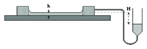
Figure 1: Diagram of the technique for determining the disjoining pressure isotherms of wetting films on a solid substrate: a circular wetting film is formed on a flat substrate to which a microporous filter with a cylindrical hole is clamped. A pipe connects the filter filled with the liquid to a reservoir containing the liquid mother bulk that can be moved by a micrometric device. The disjoining pressure is equal to $\Pi=(\rho_{b}-\rho_{{v_{b}}})\,gH$ (From Ref. [3], page 332).

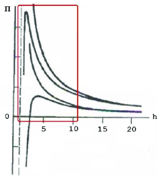
Figure 2: Experimental curves of the disjoining pressure (issued from Ref. [31]): the h-axis unit is the nanometer; the $\Pi$-axis unit is about some atmospheres. The rectangle area corresponds to a domain where the curves of the disjoining pressure (which depends on the quality of the wall) do not have a behavior as $\,h^{-3}$ like in classical theory of thin films [19]. This experimental behavior corresponds to nanofilms of a very few number of nanometers. This behavior is similar to the one obtained from our model of functional which takes into account both wall and liquid-vapor interface effects.

Clearly, the disjoining pressure could be measured by applying an external pressure to keep the layer in equilibrium. The measure of the disjoining pressure is either the additional pressure on the surface or the drop in the pressure within the mother bulks that produce the layer. In both cases, the forces arising during the thinning of a film of uniform thickness $h$ produce the disjoining pressure $\Pi(h)$ of the layer with the surrounding phases; the disjoining pressure is equal to the difference between the pressure $P_{{v_{b}}}$ on the interfacial surface (which is the pressure of the vapor mother bulk of density $\rho_{v_{b}}$) and the pressure $P_{b}$ in the liquid mother bulk (density $\rho_{b}$) from which the layer extends:

$$\Pi(h)=P_{{v_{b}}}-P_{b}\,.$$

The most classical apparatus to measure the disjoining pressure is due to Sheludko [30] and is described on Fig. (1). The film is so thin that the gravity effect is neglected across the layer. Experimental curves of the disjoining pressure were first obtained by Derjaguin. The behavior of the disjoining pressure for a nanofilm in [31] seems strongly different from the one obtained for thin liquid film in [19] (see Fig. 2).
If $g_{b}(\rho)=g_{o}(\rho)-g_{o}(\rho_{b})-\mu_{o}(\rho_{b})(\rho-\rho_{b})$ denotes the primitive of $\mu_{b}(\rho)$, null for $\rho_{b}$, we get from Eq. (10)

$$\Pi(\rho_{b})=-g_{b}(\rho_{v_{b}}),$$ (15)

and an integration of Eq. (11) yields

$$\frac{\lambda}{2}\,\left(\frac{d\rho}{dz}\right)^{2}=g_{b}(\rho)+\Pi(\rho_{b}).$$ (16)

The reference chemical potential linearized near $\rho_{l}$ (respectively $\rho_{v}$) is $\ \mu_{o}(\rho)=\displaystyle\frac{c_{l}^{2}}{\rho_{l}}(\rho-\rho_{l})\$ $\left(\emph{respectively}\ \mu_{o}(\rho)=\displaystyle\frac{c_{v}^{2}}{\rho_{v}}(\rho-\rho_{v})\right)$ where $c_{l}$ (respectively $c_{v}$) is the isothermal sound velocity in liquid bulk $\rho_{l}$ (respectively vapor bulk $\rho_{v}$) at temperature $\theta$ [32]. In the liquid and vapor parts of the liquid-vapor film, Eq. (11) yields

$$\lambda\frac{d^{2}\rho}{dz^{2}}=\frac{c_{l}^{2}}{\rho_{l}}(\rho-\rho_{b})\quad\mathrm{(liquid)}\quad\mathrm{and}\quad\lambda\frac{d^{2}\rho}{dz^{2}}=\frac{c_{v}^{2}}{\rho_{v}}(\rho-\rho_{v_{b}})\quad\mathrm{(vapor)}.$$

The values of $\mu_{o}(\rho)$ are equal for the mother densities $\rho_{v_{b}}$ and $\rho_{{b}}$,

$$\frac{c_{l}^{2}}{\rho_{l}}(\rho_{b}-\rho_{l})=\mu_{o}(\rho_{b})=\mu_{o}(\rho_{v_{b}})=\frac{c_{v}^{2}}{\rho_{v}}(\rho_{v_{b}}-\rho_{v}),\ \ \mathrm{and\ consequently,}$$

$$\rho_{v_{b}}=\rho_{v}\left(1+\frac{c_{l}^{2}}{c_{v}^{2}}\frac{(\rho_{b}-\rho_{l})}{\rho_{l}}\right).$$

In the liquid and vapor parts of the complete liquid-vapor layer we get the first expansion of the free energy, null when $\rho=\rho_{l}$ and $\rho=\rho_{v}$ respectively,

$$g_{o}(\rho)=\frac{c_{l}^{2}}{2\rho_{l}}(\rho-\rho_{l})^{2}\ \ \ \mathrm{(liquid)}\quad\mathrm{and}\quad g_{o}(\rho)=\frac{c_{v}^{2}}{2\rho_{v}}(\rho-\rho_{v})^{2}\ \ \ \mathrm{(vapor)}.$$

From definition of $g_{b}(\rho)$ and Eq. (15) we deduce the disjoining pressure

$$\Pi(\rho_{b})=\frac{c_{l}^{2}}{2\rho_{l}}(\rho_{l}-\rho_{b})\left[\rho_{l}+\rho_{b}-\rho_{v}\left(2+\frac{c_{l}^{2}}{c_{v}^{2}}\frac{(\rho_{b}-\rho_{l})}{\rho_{l}}\right)\right].$$ (17)

Far from the critical point, due to $\ \displaystyle\rho_{v}\left(2+\frac{c_{l}^{2}}{c_{v}^{2}}\frac{(\rho_{b}-\rho_{l})}{\rho_{l}}\right)\ll\rho_{l}+\rho_{b}$, we get $\displaystyle\ \Pi(\rho_{b})\approx\frac{c_{l}^{2}}{2\rho_{l}}(\rho_{l}^{2}-\rho_{b}^{2}).$ Now, we consider a film of thickness $h$; the density profile in the liquid part of the liquid-vapor film is solution of the differential equation,

$$\lambda\frac{d^{2}\rho}{dz^{2}}=\frac{c_{l}^{2}}{\rho_{l}}(\rho-\rho_{b})$$ (18)

$$\quad\mathrm{with}\quad\displaystyle\lambda\frac{d\rho}{dz}_{\left|{}_{z=0}\right.}=-\gamma_{1}+\gamma_{2\ }\rho_{\left|{}_{z=0}\right.}\quad\mathrm{and}\quad\displaystyle\lambda\frac{d\rho}{dz}_{\left|{}_{z=h}\right.}=-\gamma_{4}\ \rho_{\left|{}_{z=h}\right.}.$$

With defining $\tau$ such that $\displaystyle\tau={c_{l}}/\sqrt{\lambda\rho_{l}}\ ,$ where $d=1/\tau$ is a reference length and $\gamma_{3}=\lambda\tau$, the solution of Eq. (18) is

$$\rho=\rho_{b}+\rho_{1}\,e^{-\tau z}+\rho_{2}\,e^{\tau z},$$ (19)

where the boundary conditions at $z=0$ and $z=h$ yield the values of $\rho_{1}$ and $\rho_{2}$ satisfying

$$\left\{\begin{array}[]{c}(\gamma_{2}+\gamma_{3})\rho_{1}+(\gamma_{2}-\gamma_{3})\rho_{2}=\gamma_{1}-\gamma_{2}\rho_{b},\\ \quad\quad-e^{-h\tau}(\gamma_{3}-\gamma_{4})\rho_{1}+e^{h\tau}(\gamma_{3}+\gamma_{4})\rho_{2}=-\gamma_{4}\rho_{b}\,.\end{array}\right.\$$

The liquid density profile is a consequence of Eq. (19) when $z$ $\in\left[0,h\right]$,

$$\rho = \rho_{b}+\frac{(\gamma_{1}-\gamma_{2}\rho_{b})(\gamma_{3}+\gamma_{4})e^{h\tau}+(\gamma_{2}-\gamma_{3})\gamma_{4}\rho_{b}}{(\gamma_{2}+\gamma_{3})(\gamma_{3}+\gamma_{4})e^{h\tau}+(\gamma_{3}-\gamma_{4})(\gamma_{2}-\gamma_{3})e^{-h\tau}}\ e^{-\tau z}+$$ (20)

$$\frac{-(\gamma_{2}+\gamma_{3})\gamma_{4}\rho_{b}+(\gamma_{1}-\gamma_{2}\rho_{b})(\gamma_{3}-\gamma_{4})e^{-h\tau}}{(\gamma_{2}+\gamma_{3})(\gamma_{3}+\gamma_{4})e^{h\tau}+(\gamma_{3}-\gamma_{4})(\gamma_{2}-\gamma_{3})e^{-h\tau}}\ e^{\tau z}.$$

Equations (16,19) together with $g_{b}(\rho)=(c_{l}^{2}/2\,\rho_{l})(\rho-\rho_{b})^{2}$ for the liquid part of the layer yield

$$\Pi(\rho_{b})=-\frac{2\,c_{l}^{2}}{\rho_{l}}\,\rho_{1}\,\rho_{2}.$$ (21)

The disjoining pressure is an invariant through the liquid film and its value is function of both $\rho_{b}$ and $h$,

$$\Pi(\rho_{b}) = \frac{2c_{l}^{2}}{\rho_{l}}\left[(\gamma_{1}-\gamma_{2}\rho_{b})(\gamma_{3}+\gamma_{4})e^{h\tau}+(\gamma_{2}-\gamma_{3})\gamma_{4}\rho_{b}\right]\times$$ (22)

$$\frac{\left[(\gamma_{2}+\gamma_{3})\gamma_{4}\rho_{b}-(\gamma_{1}-\gamma_{2}\rho_{b})(\gamma_{3}-\gamma_{4})e^{-h\tau}\right]}{\left[(\gamma_{2}+\gamma_{3})(\gamma_{3}+\gamma_{4})e^{h\tau}+(\gamma_{3}-\gamma_{4})(\gamma_{2}-\gamma_{3})e^{-h\tau}\right]^{2}}.$$

By identification of expressions (17) and (22), we get a relation between $h$ and $\rho_{b}$. Consequently, we get a relation between the disjoining pressure $\Pi(\rho_{b})$ and the thickness $h$ of the liquid film. For the sake of simplicity, we denote the disjoining pressure as a function of $h$ at temperature $\theta$ by $\Pi=\Pi(h)$.
In experiments, for liquid in equilibrium with bubbles - even with a bubble diameter of a few number of nanometers - we have $\rho_{b}\simeq\rho_{l}$ [33]. Consequently, the disjoining pressure is expressed as a function of $h$ in the approximative form

$$\Pi(h) = \frac{2\,c_{l}^{2}}{\rho_{l}}\left[(\gamma_{1}-\gamma_{2}\rho_{l})(\gamma_{3}+\gamma_{4})e^{h\tau}+(\gamma_{2}-\gamma_{3})\gamma_{4}\rho_{l}\right]\times$$

$$\frac{\left[(\gamma_{2}+\gamma_{3})\gamma_{4}\rho_{l}-(\gamma_{1}-\gamma_{2}\rho_{l})(\gamma_{3}-\gamma_{4})e^{-h\tau}\right]}{\left[(\gamma_{2}+\gamma_{3})(\gamma_{3}+\gamma_{4})e^{h\tau}+(\gamma_{3}-\gamma_{4})(\gamma_{2}-\gamma_{3})e^{-h\tau}\right]^{2}}.$$

Let us notice an important property of the mixture of a fluid far under its critical point and a perfect gas, where the total pressure is the sum of the partial pressures of the components [32]: at equilibrium, the partial pressure of the perfect gas is constant through the liquid-vapor-gas layer where the perfect gas is dissolved in the liquid. The disjoining pressure of the mixture is the same as for a single fluid and calculations and results are identical to those previously obtained.

5 A comparison of the model with experiments

Our aim is not to propose an exhaustive study of the disjoining pressure for all physicochemical conditions associated with different fluids bounded by different walls, but to point out an example such that previous modeling appropriately fits with experimental data. At $\theta=20{{}^{\circ}}$ Celsius, we successively consider water wetting walls (a wall of silicon is the reference material) and water not wetting a wall.

Physical constants $c_{ll}$ $\sigma_{l}$ $m_{l}$ $\rho_{l}$ $c_{l}$ Water $1.4\times 10^{-58}$ $2.8\times 10^{-8}$ $2.99\times 10^{-23}$ $0.998$ $1.478\times 10^{5}$ Physical constants $c_{ls}$ $\sigma_{s}$ $m_{s}$ $\rho_{s}$ $\delta$ Silicon $1.4\times 10^{-58}$ $2.7\times 10^{-8}$ $4.65\times 10^{-23}$ $2.33$ $2.75\times 10^{-8}$ Deduced constants $\lambda$ $\gamma_{1}$ $\gamma_{2}=\gamma_{4}$ $\gamma_{3}$ $d$ Results (water-silicon) $1.17\times 10^{-5}$ $81.2$ $54.2$ $506$ $2.31\times 10^{-8}$

Table 1: The physical values associated with water and silicon are obtained in references [21, 34] and expressed in c.g.s. units (centimeter, gramme, second). No information is available for water-silicon interactions; we assume that $c_{ll}=c_{ls}$. The deduced constants are obtained from physical values by means of formulae obtained in sections 2-4.

Due to Eq. (20), Fig. 3 represents water liquid density profiles in the nanolayer. We verify the consistency of the model:
$\bullet$ The density gradient is large at a few nanometer range from the solid wall and consequently in this domain, the liquid is inhomogeneous,
$\bullet$ The boundary condition (14) is well adapted to our model of functional and determines the position where the phase transition between liquid and vapor occurs: condition (14) yields a density value of the fluid corresponding to an intermediate density which can be associated with a dividing surface separating liquid and vapor in the liquid-vapor interface. Due to the film instability, we will see further down that graph (b) in Fig. 3 is unphysical.

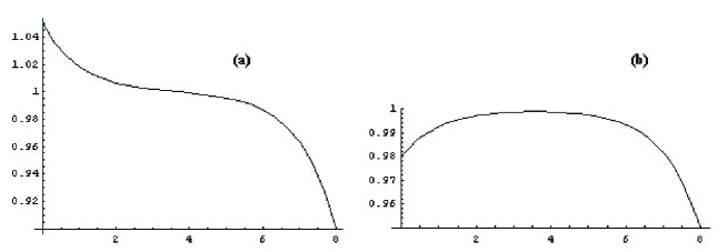
Figure 3: Graphs of liquid density profiles in a nanofilm. Results are given in two cases: Graph (a) corresponds to the case of a liquid damping a solid wall ($\gamma_{1}-\gamma_{2}\rho_{l}<0$); wetting data are associated with liquid water on silicon (cf. graph (b) in Fig. 4). Graph (b) corresponds to the unphysical case of non-wetting liquid ($\gamma_{1}-\gamma_{2}\rho_{l}>0$); non-wetting data are associated with liquid water and a wall such that $\gamma_{1}=30$, all the other deduced constants $\lambda,\gamma_{2},\gamma_{3},\gamma_{4}$ being unchanged (cf. graph (d) in Fig. 4). The unit of the $x-$axis is $\delta=2.75\times 10^{-8}$ cm (2.75 Angström), the unit of the $y-$axis is the liquid water density at 20^∘Celsius (approximatively $1$ g/cm³).

We have drawn disjoining pressure profiles deduced from analytical expressions given in section 4; the graphs relate to Rel. (22).
Graphs are associated with several cases when water damps the solid wall (at the wall, the water density is closely $\rho_{l}$ and $\gamma_{1}-\gamma_{2}\rho_{l}>0$) and a case when water does not damp the solid wall ($\gamma_{1}-\gamma_{2}\rho_{l}<0$).

Values of $\gamma_{1}$ $110$ $81.2$ $58$ $30$ Corresponding graphs in Fig. 4 (a) (b) (c) (d)

Table 2: The numerical data $\lambda,\gamma_{2},\gamma_{3},\gamma_{4}$ corresponding to liquid water are unchanged. They have the values presented in Table 1. Only the values of $\gamma_{1}$ (in c.g.s. units) depending on the behavior of the solid walls are different following graphs (a), (b), (c), (d) drawn in Fig. 4.

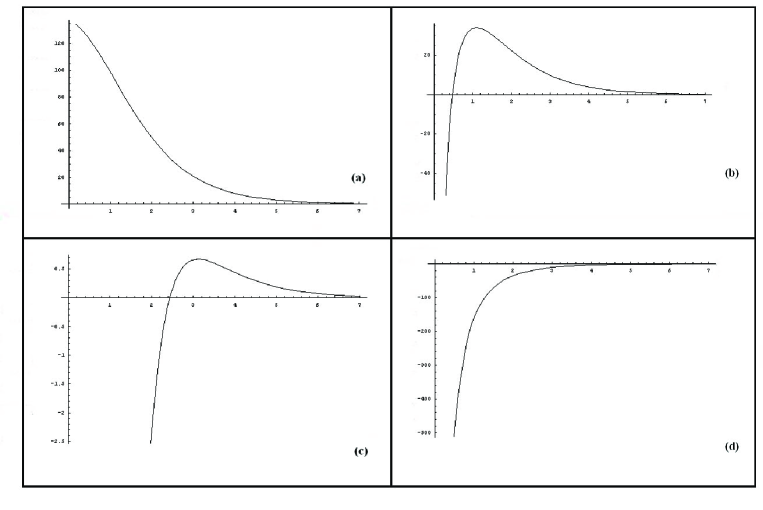
Figure 4: Several graphs represent the disjoining pressure for liquid water at $20{{}^{\circ}}$ C in contact with different plane solid walls: graphs (a), (b), (c) correspond to water damping the wall; graph (d) corresponds to an unphysical case of water not damping the wall. The unit of the $x-$axis is $\delta$, the unit of the $y-$axis is $10^{6}\ Barye$ (one atmosphere).

According to different physical values, graphs (a), (b) and (c) of Fig. (4) represent the disjoining pressure profiles for water in contact with a plane solid wall at $20{{}^{\circ}}$ Celsius.
Graph (b) corresponds to a silicon solid wall. Graphs (a) and (c) respectively correspond to water wetting more strongly the wall than a silicon wall and water wetting less strongly the wall than a silicon wall.
In [5], we studied the stability of nanofilm. In accordance with results in [3], Graph (a) is associated with a stable nanolayer for any liquid film thickness because for all $\displaystyle{\ h,\ \partial\Pi(h,\theta)}/{\partial h}<0$. In graphs (b) and (c), values of $h$ for which the liquid nanolayer is stable correspond to a domain where $\displaystyle{\ \partial\Pi(h,\theta)}/{\partial h}<0$, corresponding to $h$ values greater than a particular value $h_{s}$ depending on $\gamma_{1}$.
Graph (d) differs from previous ones as that liquid water does not damp the solid wall. The graph corresponds to an unstable nanolayer and does not exist physically. In the non-wetting case, liquid nanolayers are unstable and they are associated with compression instead of suction in experiments by Sheludko [30].
We notice that graphs (a), (b), (c) in Fig. 4, experimental graph in Fig. 2 and graphs in experimental literature (as in [3, 31]) exhibit quite similar behaviors.

6 Conclusion

We have studied liquid nanofilms in contact with plane solid walls. For layer thicknesses of some nanometers, the theoretical graphs of the disjoining pressure correctly draw the behavior of experiments by Derjaguin and others [3, 30]. The proposed analytical method is different from Lifschitz one in which layers were considered with uniform density liquids [19]. In our model corresponding to thin liquid nanofilms, liquids are considered as inhomogeneous near the solid walls. The density distribution in liquid nanofilms depends on the physicochemical characteristics of walls: when the liquid damps the wall, we have an excess of fluid density at the wall and the fluid is denser at the wall than in the liquid bulk; the contrary happens when the liquid does not damp the wall.
These analytical results and the liquid density profiles are in accordance with experimental works by Derjaguin and others [3, 4, 11].

References

- [1] B. Bhushan, Springer Handbook of Nanotechnology, Springer, Berlin, 2004.
- [2] B.V. Derjaguin, V.V. Karasev, E.N. Khromova, Thermal expansion of water in fine pores, J. Colloid Interface Sci. 109 (1986) 586 - 587.
- [3] B.V. Derjaguin, N.V. Chuarev, V.M. Muller, Surfaces Forces, Plenum Press, New York (1987).
- [4] D. Green-Kelly, B.V. Derjaguin, in Research in Surfaces Forces, vol. 2, Consultants Bureau, New York (1966) p. 117.
- [5] H. Gouin, S. Gavrilyuk, Dynamics of liquid nanofilms, Int. J. Eng. Sci. 46 (2008) 1195 - 1202.
- [6] J.E. Dunn, R. Fosdick, M. Slemrod, Eds., Shock induced transitions and phase structures, The IMA Volumes in Mathematics and its Applications 52, 1993.
- [7] P. Seppecher, Moving contact lines in the Cahn-Hilliard theory, Int. J. Eng. Sci 34 (1996) 977 - 992.
- [8] B. Widom, What do we know that van der Waals did not know?, Physica A 263 (1999) 500 - 515.
- [9] B. Kazmierczak, K. Piechór, Parametric dependence of phase boundary solution to model kinetic equations, ZAMP 53 (2002) 539 - 568.
- [10] A. Onuki, Dynamic van der Waals theory, Phys. Rev. E 75 (2007) 036304.
- [11] A.A. Chernov, L.V. Mikheev, Wetting of solid surfaces by a structured simple liquid: effect of fluctuations, Phys. Rev. Lett, 60 (1988) 2488 - 2491.
- [12] V.C. Weiss, Theoretical description of the adsorption and the wetting behavior of alkanes on water, J. Chem. Phys. 125 (2006) 084718.
- [13] R. Evans, The nature of liquid-vapour interface and other topics in the statistical mechanics of non-uniform classical fluids, Adv. Phys. 28 (1979) 143 - 200.
- [14] M.E. Fisher, A.J. Jin, Effective potentials, constraints, and critical wetting theory, Phys. Rev. B, 44 (1991) 1430 - 1433.
- [15] J.S. Rowlinson, B. Widom, Molecular Theory of Capillarity, Clarendon Press, Oxford, 1984.
- [16] H. Nakanishi, M.E. Fisher, Multicriticality of wetting, prewetting, and surface transitions, Phys. Rev. Lett. 49 (1982) 1565 - 1568.
- [17] J.W. Cahn, Critical point wetting, J. Chem. Phys. 66 (1977) 3667 - 3672.
- [18] H. Gouin, Energy of interaction between solid surfaces and liquids, J. Phys. Chem. B 102 (1998) 1212 - 1218.
- [19] I.E. Dzyaloshinsky, E.M. Lifshitz, L.P. Pitaevsky, The general theory of van der Waals forces, Adv. Phys. 10 (1961) 165 - 209.
- [20] Y. Rocard, Thermodynamique, Masson, Paris, 1952.
- [21] J. Israelachvili, Intermolecular Forces, Academic Press, New York, 1992.
- [22] H.C. Hamaker, The London-van der Waals attraction between spherical particles, Physica 4, (1937) 1058 - 1072.
- [23] P.G. de Gennes, Wetting: statics and dynamics, Rev. Mod. Phys. 57, (1985), 827 - 863.
- [24] S. Gavrilyuk, I. Akhatov, Model of a nanofilm on a solid substrate based on the van der Waals concept of capillarity, Physical Review E 73 (2006) 021604.
- [25] L.M. Pismen, Y. Pomeau, Disjoining potential and spreading of thin liquid layers in the diffuse-interface model coupled to hydrodynamics, Phys. Rev. E 62 (2000) 2480 - 2492.
- [26] J. Serrin, Mathematical principles of classical fluid mechanics, in: S. Flügge (Ed.), Encyclopedia of Physics VIII/1, Springer, Berlin, 1960.
- [27] H. Gouin, Utilization of the second gradient theory in continuum mechanics to study the motion and thermodynamics of liquid-vapor interfaces, Physicochemical Hydrodynamics, B Physics 174 (1987) 667 - 682.
- [28] H. Gouin, W. Kosiński, Boundary conditions for a capillary fluid in contact with a wall, Arch. Mech. 50 (1998), 907 - 916.
- [29] H. Gouin, S. Gavrilyuk, Wetting problem for multi-component fluid mixtures, Physica A 268 (1999) 291 - 308.
- [30] A. Sheludko, Thin liquid films, Adv. Colloid Interface Sci. 1 (1967) 391 - 464.
- [31] B.V. Derjaguin, B.V. Chuarev, Wetting Films, Nauka, Moscow (1984) in Russian.
- [32] H. Gouin, L. Espanet, Bubble number in a caviting flow, Comptes Rendus Acad. Sci. Paris 328 IIb (2000) 151 - 157.
- [33] F. dell’Isola, H. Gouin, G. Rotoli, Nucleation of spherical shell-like interfaces by the second gradient theory: numerical simulations, Eur. J. Mech, B/Fluids 15 (1996) 545 - 568.
- [34] Handbook of Chemistry and Physics, 65th Edition, CRC Press, Boca Raton, 1984/1985.