The Pt isotopes: comparing the Interacting Boson Model with Configuration Mixing and the Extended Consistent-Q formalism

Abstract

The role of intruder configurations in the description of energy spectra and $B(E2)$ values in the Pt region is analyzed. In particular, we study the differences between Interacting Boson Model calculations with or without the inclusion of intruder states in the even Pt nuclei ^172-194Pt. As a result, it shows that for the description of a subset of the existing experimental data, i.e., energy spectra and absolute $B(E2)$ values up to an excitation energy of about $1.5$ MeV, both approaches seem to be equally valid. We explain these similarities between both model spaces through an appropriate mapping. We point out the need for a more extensive comparison, encompassing a data set as broad (and complete) as possible to confront with both theoretical approaches in order to test the detailed structure of the nuclear wave functions.

PACS: 21.10.-k, 21.60.-n, 21.60.Fw.

Keywords: Pt isotopes, shape coexistence, intruder states, energy fits.

1 Introduction

The appearance of shape coexistence in nuclei has attracted a lot of attention in recent decades [1, 2, 3] and compelling evidence has been obtained, in particular, at and very near to proton or neutron closed shells. The Pb region takes a prominent position because in addition to specific shell-model excitations established close to the $N=126$ neutron shell closure, collective excitations have been observed for the neutron-deficient nuclei [4]. The review paper of Julin et al. [3] gives an extensive overview of the rich variety in nuclear excitation modes for both the Pb, Hg, Pt and, Po, Rn nuclei. Since the publication of that paper, however, many experiments have been performed highlighting properties of excited band structures and lifetimes for the Pb nuclei [5, 6, 7, 8, 9, 10, 11, 12, 13] and nearby nuclei, also illuminating the underlying mechanisms that are at the origin of the formation of collective excitations in the neutron-deficient nuclei near to the $Z=82$ proton closed shell.

This mass region has been studied theoretically in an extensive way. Early calculations using a deformed Woods-Saxon potential in order to explore the nuclear energy surfaces as a function of the quadrupole deformation variables [14, 15, 16, 17] showed a consistent picture pointing out the presence of oblate and prolate energy minima. More recently, mean-field calculations going beyond the static part, including dynamical effects using the Generator Coordinate Method (GCM) [18], either starting from Skyrme functionals [13, 19, 20, 21], or using the Gogny D1S parametrization [22, 23, 24, 25, 26] have put the former calculations on firm ground and have also given rise to detailed information of the collective bands observed in neutron-deficient nuclei around the $Z=82$ closed proton shell. Here, we should also mention attempts to study shape transitions in the Os and Pt nuclei within the relativistic mean field (RMF) approach [27].

¿From a microscopic shell-model approach, the hope to treat on equal footing the large open neutron shell from $N=126$ down to and beyond the mid-shell $N=104$ region, with valence protons in the Pt, Hg, Po, and Rn nuclei, and even including proton multi-particle multi-hole (mp-nh) excitations across the $Z=82$ shell closure, is far beyond present computational possibilities. The truncation of the model space, however, by concentrating on nucleon pair modes (mainly $0^{+}$ and $2^{+}$ coupled pairs, to be treated as bosons within the Interacting Boson Approximation (IBM) [28]), has made the calculations feasible, even including pair excitations across the $Z=82$ shell closure [29] in the Pb region. More in particular, the Pb nuclei have been extensively studied giving rise to bands with varying collectivity depending on the nature of the excitations treated in the model space [11, 30, 31, 32, 33, 34, 35, 36, 37].

In view of the fact that near the mid-shell point of the valence neutron major shell $82-126$ ($N=104$) clear-cut examples (see the discussion before) of coexisting collective bands have been observed in both the Pb ($Z=82$) and Hg ($Z=80$) isotopes, it is of the utmost importance to study the propagation of these coexisting structures as one gradually moves away from the $Z=82$ proton closed shell. Therefore, detailed studies for both the Pt, Os,… isotopes ($Z=78,76$,…) and the Po, Rn,… isotopes ($Z=84,86$,…) are of major importance in order to explore the evolution from coexisting spherical and deformed structures at the closed shell towards the onset of normal, open-shell deformation. In order to gain insight into this transition, one should, in particular, study those observables that are sensitive to specific mp-nh excitations such as the appearance of distinct collective bands making use, in particular, of Coulomb excitation with radioactive beams, $\alpha$-decay hindrance factors, isotopic shifts, E0 decay properties, g-factors. Moreover, data on low-lying excited states in the adjacent odd-proton mass Au, Tl, Bi,… isotopes as well as in the odd-neutron mass Pt, Hg, Pb, Po, Rn isotopes should allow to explore the importance of particular single-particle excitations in this mass region. The Pt nuclei form a most important set of isotopes in order to study the above question.

In the present paper, we reanalyze the Pt nuclei, motivated by the above questions and recent IBM calculations [38, 39] without explicitly including intruder excitations into the model space, considering the 4 proton holes and the number of valence neutrons with the boson model approximation. Before, it has been suggested by Wood [40, 41] that proton 6h-2p configurations must be considered, besides the regular proton 4h configurations, in order to describe the experimental data in the Pt and adjacent nuclei, in particular the sudden lowering of the first excited $0^{+}_{2}$ down to mass number $A=186$ associated with a specific change in the excitation energy for the first excited $2^{+}_{1}$ state in the same mass interval. Thus, it becomes clear that the Pt nuclei form a most important series of isotopes in order to study the above question. More specifically, within the IBM configuration-mixing approach [29] (IBM-CM for short), calculations have been carried out for the Pt nuclei by Harder et al. [42] and by King et al. [43] describing the low-lying excited states in the ^168-196Pt nuclei. In the latter studies, also $g(2^{+}_{1})$ factors and isotopic shifts were calculated and shown to be in good agreement with the known data [44, 45]. However, no $B(E2)$ values, which constitute an important test, were calculated.

We should mention that the even-even Pt around mass number $A\approx 190$ have been studied before in the framework of the proton-neutron interacting boson model by Bijker et al. [46]. They calculated a large number of observables such as the energy spectra, various ratios of reduced $E2$ transition probabilities, absolute $B(E2)$ values and quadrupole moments, two-nucleon transfer reaction intensities, isotopic and isomeric shifts and E0 transition rates. In view of the fact that this study dates back to 1980, an extensive set of new data have become available since. This warrants an in-depth study of the Pt nuclei, spanning the region from the heavier Pt nuclei (around $A\approx 196,198$) into the lightest Pt nuclei near A $\approx$ 172.

In the present study, we show that for the excited states below an excitation energy of $E_{x}\approx 1.5$ MeV, the IBM calculations with or without including explicitly particle-hole excitations reproduce equally well the excitation energies and absolute $B(E2)$ values of known states in the mass region $172\leq A\leq 194$. How then can we interpret a possible equivalence of the energies, and the $B(E2)$ values for a limited number of states, below $1.5$ MeV between both calculations? This excitation energy approximately marks the start of a region in which a unique comparison between a specific experimental level and a particular level in the IBM calculations becomes difficult to be made. First of all, we point out that even though the Hilbert spaces of both models are largely different, due to the limited number of states below $1.5$ MeV, it is not possible to discriminate between the models considering only excitation energies and $B(E2)$ values. Secondly, we point out that the difference in the Hamiltonians can result from a renormalization of the interaction. We also show that, moving towards higher-lying levels, clear differences appear between the model spaces. Moreover, we explore theoretical possibilities to understand the fact that excitation energies and electromagnetic quadrupole properties ($B(E2)$ values and quadrupole moments) exhibit a very strong ressemblance, although originating from highly different wave functions. In a forthcoming paper, we shall present the results of a comparison covering an as complete as possible data set (encompassing also $\alpha$-decay hindrance factors, $g(2^{+}_{1})$ factors, isotopic shifts, E0 decay properties, and also properties of the energy spectra of adjacent odd-mass Pt and Au nuclei) with the two theoretical approaches, i.e., considering a reduced model space versus an enlarged model space including particle-hole excitations, within the Interacting Boson Model context.

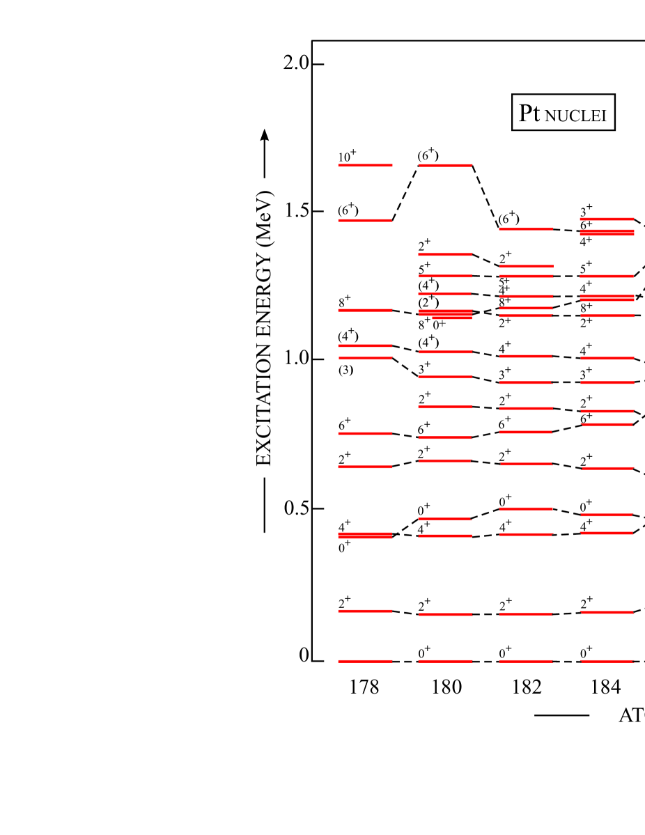
Figure 1: Energy level systematics for Pt isotopes. Only levels up to $E_{x}\sim$ 1.5 MeV are shown.

2 The experimental data in the even-even Pt nuclei

The even-even Pt nuclei, in particular the region of neutron-deficient isotopes situated around and even beyond $N=104$ neutron number ($A=182$), spanning the mass interval $172\leq A\leq 194$, have been extensively studied over the last decades. Information was taken from the appropriate Nuclear Data Sheets covering the above Pt mass region for $A=172$ [47], $A=174$ [48], $A=176$ [49], $A=178$ [50], $A=180$ [51], $A=182$ [52], $A=184$ [53], $A=186$ [54], $A=188$ [55], $A=190$ [56], $A=192$ [57] and, $A=194$ [58]. Moreover, we also incorporate data on those even-even Pt nuclei that have been published (see below) since the latest updates of the corresponding Nuclear Data Sheets.

The very light Pt nuclei with $A=168,170$ were studied by King et al. [43] using $\alpha$-decay recoil tagging gamma spectroscopy. In the case of ¹⁷⁰Pt, a ground-state band up to spin $(8^{+})$ was established. Cederwall et al. [59] obtained yrast bands for both ^171,172Pt up to spin $(25/2^{+})$ and $(8^{+})$, respectively. Seweryniak et al. [60] also studied the ^170,171,172Pt nuclei and in the case of $A=172$ could extend the yrast band structure up to spin $(14^{+})$, using recoil decay tagging. More recently, Joss et al. [61] studied the neutron-deficient ^169-173Pt nuclei obtaining more detailed information on the yrast bands for mass $A=170$ and $A=172$, and obtaining first information on side bands. Extra information on ¹⁷⁴Pt [62] and ¹⁷⁸Pt [63] has been obtained making use of the Gammasphere array, in particular, extending the yrast band up to spins $(26^{+})$ and $(24^{+})$, respectively. The yrast band in ¹⁷⁸Pt was extended by Soramel et al. [64] up to spin $(18^{+})$ using fusion-evaporation reactions. Popescu et al. [65], have studied the high-spin states (up to spin $26^{+}$) as well as the band structures in ¹⁸²Pt. A very detailed study was performed by Davidson et al. [66] via $\beta^{+}/EC$ decay using a gamma array to obtain both, yrast and non-yrast structures covering the ^176-182Pt nuclei. In particular, the data for $A=178$ and $A=182$ extend the information compiled in the corresponding Nuclear Data Sheets [50] and [52], respectively. In ¹⁸⁰Pt, lifetime measurements have been performed that allow to extract the $B(E2;4^{+}_{1}\rightarrow 2^{+}_{1})$ value. The experiment of De Voigt et al. [67] results in a value of 140$\pm$30 W.u. A more recent experiment by Williams et al. [68] has resulted in a much larger $B(E2)$ value of 260$\pm$32 W.u. thus giving rise to non-overlapping data. The mass $A=184$ Pt nucleus was studied by Xu et al. [69] in great detail, making use of the $\beta$ decay of ¹⁸⁴Au. Using both conversion electron and $\gamma$-ray spectroscopy as well as $\gamma$-ray angular distribution measurements on low-temperature oriented (LTNO) ¹⁸⁴Au nuclei, E0 $\rho^{2}$ values could be extracted demonstrating coexisting K=0 and K=2 bands. The high-spin states in ¹⁹²Pt nucleus have been studied quite recently by Oktem et al. [70], going up to spin $(20^{+})$, and by McCutchan et al. [71] studying low-spin states in ¹⁹²Pt populated in $\beta^{+}$/EC decay of ¹⁹²Au(1^-). Coulomb excitation experiments on ¹⁹⁴Pt by Wu et al. [72] have resulted in an extensive set of reduced E2 matrix elements for the ground-band, the K=2 band (encompassing both transition and diagonal matrix elements) as well as for E2 transitions decaying from the $0^{+}_{2,4}$ states.

The experimental energy systematics for the Pt nuclei, including the region of interest which is mainly situated around the neutron $N=104$ mid-shell number, is shown in Fig. 1 and spans the interval $178\leq A\leq 198$. The systematics is limited to levels with an excitation energy up to $E_{x}\approx 1.5$ MeV (a limited number of higher-spin states are given beyond this cut-off) and will serve as a “basis” to compare with the calculations described in section 3. This figure is based on the information available in the appropriate Nuclear Data Sheets, enlarged or improved including the more recent papers discussing these particular even-even Pt nuclei. Figure 1 is characterized by a sudden drop of the first excited $0^{+}_{2}$ state, down to mass $A=186$, remaining essentially constant for lower mass numbers (down to mass $A=178$). The energy spectrum remains remarkably constant in the mass interval $178\leq A\leq 186$, contrasting with a different structure that shows a number of up sloping levels with increasing mass number $A$ beyond mass $A=186$.

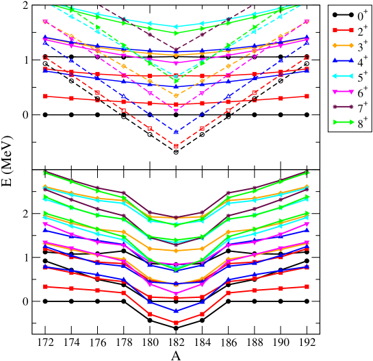
Figure 2: Excitation energies resulting from an IBM-CM Hamiltonian, using the parameters taken from Harder et al. [42]. Full lines with closed symbols correspond to the regular states, while dashed lines with open symbols correspond to the intruder states. Upper panel: calculation without the mixing term, relative to the first regular $0^{+}$ configuration. Lower panel: calculation including the mixing term with a strength equal to $50$ keV, relative to the $0^{+}$ state with the highest percentage of the regular N-boson subspace.

3 Comparing the Interacting Boson Model with configuration mixing and the extended Consistent-Q formalism

3.1 The formalism

In the present study we compare calculations carried out within the context of the IBM, incorporating 2p-2h excitations across the $Z=82$ proton closed shell into the model space (also called IBM-configuration mixing, or IBM-CM as a shorthand notation), with recent studies using the standard IBM in which excitations across the $Z=82$ core are not included explicitly.

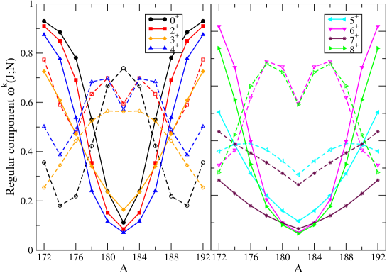
Figure 3: The regular configuration content, expressed by the weight $w^{k}(J,N)$ (see text), for the two lowest-lying states $(k=1,2)$ (full lines with closed symbols are used for the first state while dashed lines with open symbols are used for the second state) for each of the angular momenta $0^{+},2^{+},3^{+},4^{+},5^{+},6^{+},7^{+},8^{+}$, corresponding to the lower panel of Fig. 2.

The IBM-CM allows the simultaneous treatment and mixing of several boson configurations which correspond to different particle–hole (p–h) shell excitations [29]. On the basis of intruder spin symmetry [33, 73], no distinction is made between particle and hole bosons. Hence, the model space which includes the regular proton 4h configurations and a number of valence neutrons outside of the $N=82$ closed shell (corresponding to the standard IBM treatment for the Pt even-even nuclei) as well as the proton 6h-2p configurations and the same number of valence neutrons corresponds to a $[N]\oplus[N+2]$ boson space ($N$, being the number of active protons, counting both, proton holes and particles, plus the number of valence neutrons outside the $N=126$ or the $N=82$ closed shell (depending on the nearest closed shell), divided by $2$ as the boson number). Consequently, the Hamiltonian for two-configuration mixing can be written as

$$\hat{H}=\hat{P}^{{\dagger}}_{N}\hat{H}^{N}_{\rm ecqf}\hat{P}_{N}+\hat{P}^{{\dagger}}_{N+2}\left(\hat{H}^{N+2}_{\rm ecqf}+\Delta^{N+2}\right)\hat{P}_{N+2}\ +\hat{V}_{\rm mix}^{N,N+2}~{},$$ (1)

where $\hat{P}_{N}$ and $\hat{P}_{N+2}$ are projection operators onto the $[N]$ and the $[N+2]$ boson spaces, respectively, $\hat{V}_{\rm mix}^{N,N+2}$ describes the mixing between the $[N]$ and the $[N+2]$ boson subspaces, and

$$\hat{H}^{i}_{\rm ecqf}=\varepsilon_{i}\hat{n}_{d}+\kappa^{\prime}_{i}\hat{L}\cdot\hat{L}+\kappa_{i}\hat{Q}(\chi_{i})\cdot\hat{Q}(\chi_{i}),$$ (2)

is the extended consistent-Q Hamiltonian (ECQF) [74] with $i=N,N+2$, $\hat{n}_{d}$ the $d$ boson number operator,

$$\hat{L}_{\mu}=[d^{\dagger}\times\tilde{d}]^{(1)}_{\mu},$$ (3)

the angular momentum operator, and

$$\hat{Q}_{\mu}(\chi_{i})=[s^{\dagger}\times\tilde{d}+d^{\dagger}\times s]^{(2)}_{\mu}+\chi_{i}[d^{\dagger}\times\tilde{d}]^{(2)}_{\mu}~{},$$ (4)

the quadrupole operator. We are not considering the most general IBM Hamiltonian in each Hilbert space, [N] and [N+2], but we are restricting ourselves to an ECQF formalism [74, 75] in each subspace. This approach has been shown to be a rather good approximation in many calculations.

The parameter $\Delta^{N+2}$ can be associated with the energy needed to excite two particles across the $Z=82$ shell gap, corrected for the pairing interaction gain and including monopole effects [30, 76]. The operator $\hat{V}_{\rm mix}^{N,N+2}$ describes the mixing between the $N$ and the $N+2$ configurations and is defined as

$$\hat{V}_{\rm mix}^{N,N+2}=w_{0}^{N,N+2}(s^{\dagger}\times s^{\dagger}+s\times s)+w_{2}^{N,N+2}(d^{\dagger}\times d^{\dagger}+\tilde{d}\times\tilde{d})^{(0)}.$$ (5)

The wave function in the IBM-CM can then be described as follows

$$\Psi(k,JM) = \sum_{i}a^{k}_{i}(J;N)\psi((sd)^{N}_{i};JM)$$ (6)

$$+ \ \sum_{j}b^{k}_{j}(J;N+2)\psi((sd)^{N+2}_{j};JM)~{}.$$

The $E2$ transition operator for two-configuration mixing is subsequently defined as

$$\hat{T}(E2)_{\mu}=\sum_{i=N,N+2}e_{i}\hat{P}_{i}^{\dagger}\hat{Q}_{\mu}(\chi_{i})\hat{P}_{i}~{},$$ (7)

where the $e_{i}$ ($i=N,N+2$) are the effective boson charges and $\hat{Q}_{\mu}(\chi_{i})$ is the quadrupole operator defined in Eq. (4).

The starting point of the present IBM-CM mixing analysis is the work by Harder et al. [42], in which a schematic IBM mixing calculation with a fixed Hamiltonian along the whole chain of the Pt nuclei was carried out. The parameters used in that calculation are presented in Table 1.

	$\varepsilon_{i}$	$\kappa^{\prime}_{i}$	$\kappa_{i}$	$\chi_{i}$	$e_{i}$
$N$	540	0	-27	0.25	0.16
$N+2$	0	10	-22	-0.45	0.13

Table 1: Hamiltonian and $\hat{T}(E2)$ parameters from Harder et al. [42]. All the quantities are given in keV, except for $\chi_{i}$ which are dimensionless and for the effective charges, $e_{i}$, which are given in e$\cdot$b. The remaining parameters of the Hamiltonian are: $\Delta^{N+2}=1400$ keV and $w_{0}^{N,N+2}=w_{2}^{N,N+2}=50$ keV.

Although these calculations were able to reproduce the evolution of the structure of the low-lying states in a qualitative way, they do not allow for a reproduction of the finer details. Besides, $B(E2)$ values have not been calculated in that study. In Fig. 2, we represent the major results from [42], in particular the excitation energies, first without the mixing term and relative to the first regular $0^{+}$ state (upper panel) in which the behavior of the regular and intruder states stands out clearly, and secondly, including a mixing term equal to $50$ keV (lower panel). In the lower panel of the figure, the energies are given relative to the $0^{+}$ state with the highest percentage of the regular N-boson subspace. In Fig. 3 we represent that part of the wave function contained within the N-boson subspace, defined as the sum of the squared amplitudes, or weight $w^{k}(J,N)\equiv\sum_{i}\mid a^{k}_{i}(J;N)\mid^{2}$, of the two lowest-lying states $(k=1,2)$ for the most important angular momentum values that show up in the low-energy spectrum corresponding to the lower panel of Fig. 2.

Several features are highlighted by inspection of Figs. 2 and 3. First of all, one observes a rapid change in the structure of the states, with the lowest states resulting as mainly regular at the beginning (end) of the shell, while the intruder character becomes dominant at the mid-shell, $A=182~{}(N=104)$ region. The first state for each $L$ is mainly regular at the beginning (end) of the shell, while mainly intruder at the mid-shell. For the second state the situation is rather the opposite. It is mainly an intruder state at the beginning (end) of the shell, while regular at the mid-shell region. In the case of the $5^{+}$ and $7^{+}$ states, they behave over the whole mass-range as intruder states, with a minimal content of the regular component at the mid-shell. Secondly, the energy spectra are symmetric with respect to the mid-shell point at $N=104$ with an unrealistic kink appearing at the mid-shell position, while the real data do not exhibit such a pronounced behavior. As a conclusion, it turns out that one would need a strong mixing term in order to approximately reproduce the experimental data. Finally, it becomes clear that the parameters from [42] should be fine tuned in order to reproduce the experimental data (excitation energy and $B(E2)$ values) quantitatively.

An alternative method to analyze this mass region was proposed recently by McCutchan et al. [38], in which the Pt nuclei were treated as consisting of just four proton holes and a number of valence neutrons, moving outside of the $Z=82$, $N=82$ doubly-closed shell. Thus, proton excitations across the $Z=82$ closed shell were not taken into account explicitly. In this single-space approach, considering $N$ bosons, McCutchan et al. used the ECQF [74, 75] with the Hamiltonian [77]

$$\hat{H}(\zeta)=c((1-\zeta)\hat{n}_{d}-\frac{\zeta}{4N}\hat{Q}(\chi).\hat{Q}(\chi))~{},$$ (8)

where the quadrupole operator is given by Eq. (4). The parameter $c$ is a general energy scaling factor, $N$ is the number of s and d bosons and $\zeta$ and $\chi$ are two structural parameters, describing the spherical-deformed transition and the prolate-oblate transition, respectively. Note that this Hamiltonian can also be rewritten using the parameters $\varepsilon_{d}$ and $\kappa$ (see equation (2)).

In the present case, one considers a limited number of basis states, i.e., only the components with $N$ bosons. This basis spans the smaller model space and the corresponding model wave function can be expressed as

$$\Psi^{\prime}(k,JM)=\sum_{l}a^{\prime k}_{l}(J;N)\psi((sd)^{N}_{l};JM)~{}.$$ (9)

In section 3.2 we present the methods used in order to determine the parameters appearing in the IBM-CM Hamiltonian as well as in the $\hat{T}(E2)$ operator. We discuss the resulting energy spectra and the $B(E2)$ reduced transition probabilities, and carry out a detailed comparison with both, the experimental data and with the ECQF calculations [38].

3.2 The fitting procedure: energy spectra and absolute $B(E2)$ reduced transition probabilities

Here, we present the way in which the parameters of the Hamiltonian (1), (2), and (5) and the effective charges in the $\hat{T}(E2)$ transition operator (7) have been determined.

In order to compare with the calculations carried out by McCutchan et al. [38], who studied besides the yrast levels, a number of non-yrast levels and the corresponding $B(E2)$ values, we have to carry out a more detailed calculation within the IBM-CM approach, going beyond the more schematic study carried out by Harder et al. [42].

We concentrate on the range ¹⁷²Pt to ¹⁹⁴Pt thereby covering a major part of the neutron $N=82-126$ shell. This interval also corresponds to the same set of isotopes analyzed in references [38] and [42].

In the fitting procedure carried out here, we try to obtain the best possible agreement with the experimental data including both the excitation energies and the $B(E2)$ reduced transition probabilities. Using the expression of the IBM-CM Hamiltonian, as given in equation (1), and of the $E2$ operator, as given in Eq. (7), in the most general case thirteen parameters show up. We impose a constraint of using parameters that change smoothly in passing from isotope to isotope. For the regular Hamiltonian, we have constrained one of the parameters, i.e., $\chi_{N}=0$, while for the intruder Hamiltonian we have fixed the relative d-boson energy to the value $\varepsilon_{N+2}=0$. These constraints follow from a number of test calculations that were carried out in which no substantial improvement in the value of $\chi^{2}$ (see Eq. (10)) was obtained if we allowed $\varepsilon_{N+2}\neq 0$ or $\chi_{N}\neq 0$. Note that the constraint $\varepsilon_{N+2}=0$ is also supported by [42]. On the other hand, we have kept the value that describes the energy needed to create an extra particle-hole pair ($2$ extra bosons) constant, i.e., $\Delta^{N+2}=1400$ keV, and have also put the constraint of keeping the mixing strengths constant, i.e., $w_{0}^{N,N+2}=w_{2}^{N,N+2}=50$ keV for all the Pt isotopes. Those parameter values have been shown to be quite appropriate in this part of the nuclear mass region [42, 43], although the choice of the mixing strength remains somewhat arbitrary [42]. We also have to determine for each isotope the effective charges of the $E2$ operator. This finally leads to eight parameters to be varied in each nucleus.

The $\chi^{2}$ test is used in the fitting procedure in order to extract the optimal solution. The $\chi^{2}$ function is defined in the standard way as

$$\chi^{2}=\frac{1}{N_{data}-N_{par}}\sum_{i=1}^{N_{data}}\frac{(X_{i}(data)-X_{i}(IBM))^{2}}{\sigma_{i}^{2}},$$ (10)

where $N_{data}$ is the number of experimental data, $N_{par}$ is the number of parameters used in the IBM fit, $X_{i}(data)$ describes the experimental excitation energy of a given experimental energy level (or an experimental $B(E2)$ value), $X_{i}(IBM)$ denotes the corresponding calculated IBM-CM value, and $\sigma_{i}$ is an error assigned to each $X_{i}(data)$ point.

The $\chi^{2}$ function is defined as a sum over all data points including excitation energies as well as absolute $B(E2)$ values. The minimization is carried out using $\varepsilon_{N}$, $\kappa^{\prime}_{N}$, $\kappa_{N}$, $\kappa^{\prime}_{N+2}$, $\kappa_{N+2}$, $\chi_{N+2}$, $e_{N}$ and $e_{N+2}$ as free parameters, having fixed $\chi_{N}=0$, $\varepsilon_{N+2}=0$, $\Delta^{N+2}=1400$ keV and $w_{0}^{N,N+2}=w_{2}^{N,N+2}=50$ keV as described before. We minimize the $\chi^{2}$ function for each isotope separately using the package MINUIT [78] which allows to minimize any multi-variable function. In some of the lighter Pt isotopes, due to the small number of experimental data, the values of some of the free parameters could not be fixed unambiguously using the above fitting procedure.

As input values, we have used the excitation energies of the levels presented in Table 2. In this table we also give the corresponding $\sigma$ values. We stress that the $\sigma$ values do not correspond to experimental error bars, but they are related with the expected accuracy of the IBM-CM calculation to reproduce a particular experimental data point. Thus, they act as a guide so that a given calculated level converges towards the corresponding experimental level. The $\sigma$ ($0.1$ keV) value for the $2_{1}^{+}$ state guarantees the exact reproduction of this experimental most important excitation energy, i.e., the whole energy spectrum is normalized to this experimental energy. As in reference [38], the states $4_{1}^{+},0_{2}^{+}$ and $2_{2}^{+}$ are considered as the most important ones to be reproduced ($\sigma=1$ keV). The group of states $4_{2}^{+},4_{3}^{+},6_{1}^{+},8_{1}^{+}$ and $3_{1}^{+}$ ($\sigma=10$ keV) and $2_{3}^{+}$ ($\sigma=100$ keV) should also be well reproduced by the calculation to guarantee a correct moment of inertia for the yrast band and the structure of the pseudo-$\gamma$ and $0_{2}^{+}$ bands. In the case of the $E2$ transition rates, we have used the available experimental data involving the states presented in Table 2, restricted to those E2 transitions for which absolute $B(E2)$ values are known. Additionally we have taken a value of $\sigma$ corresponding to $10\%$ of these $B(E2)$ values. In view of the large number of relative $B(E2)$ values, we have derived optimal effective charges using the same fitting scheme as before, but now keeping the parameters in the IBM-CM Hamiltonian fixed. Here, we include the relative $B(E2)$ values and for these data we have used a relative error of a 20%. The experimental data that we have used are taken from the Nuclear Data Sheets (NDS), Adopted Values references [47, 48, 49, 50, 51, 52, 53, 54, 55, 56, 57, 58], unless the latest issue was published more than 10 years ago. Therefore, for the mass number $A=182,184$ and $192$, the experimental data were taken from [66, 79, 71], respectively.

Precision (keV)	States
$\sigma=0.1$	$2_{1}^{+}$
$\sigma=1$	$4_{1}^{+},0_{2}^{+},2_{2}^{+}$
$\sigma=10$	$4_{2}^{+},4_{3}^{+},6_{1}^{+},8_{1}^{+},3_{1}^{+}$
$\sigma=100$	$2_{3}^{+}$

Table 2: Energy levels, characterized by $J^{\pi}_{i}$, included in the energy fit, if known, and the assigned $\sigma$ values in keV.

The fitting procedure, outlined before, has resulted in the values of the parameters for the IBM-CM Hamiltonian, as given in Table 3. Note that some of the Hamiltonian parameters, especially for ¹⁷²Pt and ¹⁷⁴Pt, remain arbitrary due to the lack of experimental data. In the case of ¹⁷²Pt and ¹⁷⁴Pt the value of the effective charges cannot be determined because not a single $B(E2)$ value is known. In the case of ¹⁸²Pt the absolute value of the effective charges cannot be determined because any absolute $B(E2)$ value is known. Therefore, the given values are dimensionless.

Nucleus	$\varepsilon_{N}$	$\kappa^{\prime}_{N}$	$\kappa_{N}$	$\kappa^{\prime}_{N+2}$	$\kappa_{N+2}$	$\chi_{N+2}$	$e_{N}$	$e_{N+2}$
172Pt	725.0	0.00	-39.47	0.00	-22.87	-0.38	-	-
174Pt	701.2	0.00	-31.60	0.00	-21.82	-0.30	-	-
176Pt	683.4	1.04	-37.62	5.24	-23.56	-0.75	1.86	1.63
178Pt	753.8	-2.31	-37.45	5.27	-25.17	-0.55	3.21	1.52
180Pt	999.3	-15.14	-37.34	6.57	-25.14	-0.32	1.29	1.94
182Pt	939.9	-6.70	-35.39	7.03	-23.50	-0.31	1	1.1
184Pt	750.6	1.47	-32.66	6.64	-23.89	-0.34	1.14	1.71
186Pt	675.3	3.17	-30.50	7.29	-24.23	-0.32	1.44	1.67
188Pt	483.2	4.94	-37.38	6.67	-31.47	-0.11	1.66	1.66
190Pt	338.7	19.33	-34.62	0.83	-32.51	0.00	1.50	1.50
192Pt	314.9	12.01	-45.32	-8.82	-38.84	0.00	1.68	1.77
194Pt	370.9	6.67	-38.26	6.52	-31.02	0.00	1.97	0.25

Table 3: Hamiltonian and $\hat{T}(E2)$ parameters resulting from the present study. All quantities have the dimension of energy (given in units of keV), except $\chi_{N+2}$ which is dimensionless and $e_{N}$ and $e_{N+2}$ which are given in units $\sqrt{\mbox{W.u.}}$, except for ¹⁸²Pt which are dimensionless (see text). The remaining parameters of the Hamiltonian, i.e., $\chi_{N}$ and $\varepsilon_{N+2}$

are equal to zero, except $\Delta^{N+2}=1400$ keV and $w_{0}^{N,N+2}=w_{2}^{N,N+2}=50$ keV.

In the ECQF fit carried out by McCutchan et al. [38], the parameters they obtained are given in Table 4 [80]. We present the values of $\zeta$ and $\chi$ and also the corresponding values of $\varepsilon$ and $\kappa$ obtained after normalizing $E(2_{1}^{+})$ to the experimental value. McCutchan et al. used the ratios $E(4_{1}^{+})/E(2_{1}^{+})$, $E(2_{\gamma}^{+})/E(2_{1}^{+})$ and $E(0_{2}^{+})/E(2_{1}^{+})$ as well as some $B(E2)$ ratios, if known, such as $B(E2;2^{+}_{2}\rightarrow 0^{+}_{1})/B(E2;2^{+}_{2}\rightarrow 2^{+}_{1})$ and $B(E2;2^{+}_{3}\rightarrow 0^{+}_{1})/B(E2;2^{+}_{3}\rightarrow 2^{+}_{1})$, in order to determine the Hamiltonian parameters as given in equation (8). The value of the effective charge of the $\hat{T}(E2)$ operator was fixed to reproduce $B(E2;2_{1}^{+}\rightarrow 0_{1}^{+})$ except for ¹⁷⁸Pt where $B(E2;4_{1}^{+}\rightarrow 2_{1}^{+})$ has been used. The ECQF fit essentially consists of four free parameters to be varied in each nucleus, separately, which is clearly less than in the IBM-CM calculations.

Nucleus	$\zeta$	$\varepsilon$	$\kappa$	$\chi$	$e$
172Pt	0.49	856.9	-25.7	-1.20	-
174Pt	0.51	811.6	-23.5	-1.10	-
176Pt	0.47	480.8	-10.7	-1.10	2.22
178Pt	0.55	472.5	-13.1	-1.00	2.09
180Pt	0.57	480.9	-13.3	-0.90	2.17
182Pt	0.57	516.3	-13.2	-0.87	-
184Pt	0.57	480.0	-13.3	-0.84	1.90
186Pt	0.59	497.0	-16.3	-0.70	1.88
188Pt	0.64	537.2	-23.9	-0.30	1.91
190Pt	0.66	526.6	-28.4	-0.20	1.70
192Pt	0.72	481.6	-38.7	-0.10	1.82
194Pt	0.74	431.3	-43.8	-0.10	1.86

Table 4: ECQF Hamiltonian parameters and $\hat{T}(E2)$ effective charge [38, 80]. All the quantities have the dimension of energy (units of keV), except $\zeta$ and $\chi$ which are dimensionless, and $e$ given in units $\sqrt{\mbox{W.u.}}$ Note that $\zeta$ is not an independent variable, but depends on $\varepsilon$ and $\kappa$.

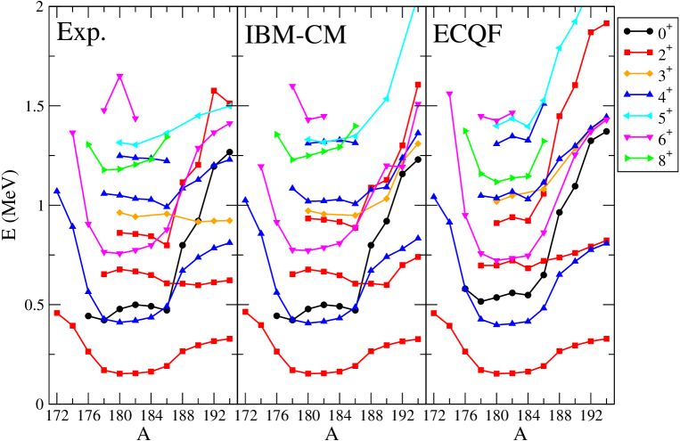
Figure 4: Experimental excitation energies (up to $E_{x}\approx 1.5$ MeV) and theoretical results obtained from the IBM-CM and ECQF calculations [38].

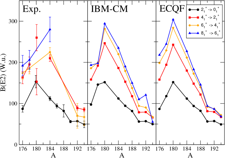
Figure 5: Comparison of a set of absolute $B(E2)$ reduced transition probabilities in the ground band, given in W.u. The left panel corresponds to known experimental data, the central panel to the theoretical IBM-CM results and the right panel to the theoretical ECQF results.

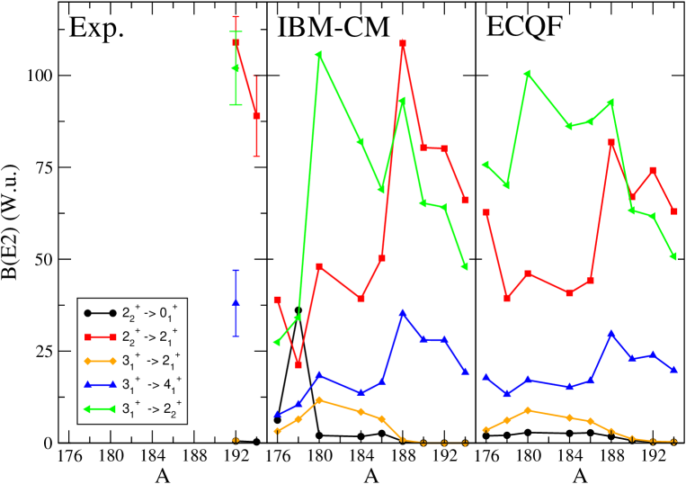
Figure 6: Comparison of a set of absolute $B(E2)$ reduced transition probabilities, given in W.u. The left panel corresponds to experimental data, the central panel to the IBM-CM results and the right panel to the ECQF results.

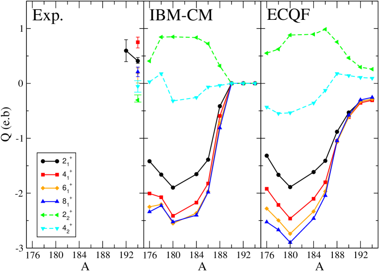
Figure 7: Comparison of the quadrupole moments for the ground band and the $2^{+}_{2},4^{+}_{2}$ states, given in units e$\cdot$b. The left panel corresponds to experimental data, the central panel to the IBM-CM results and the right panel to the ECQF results.

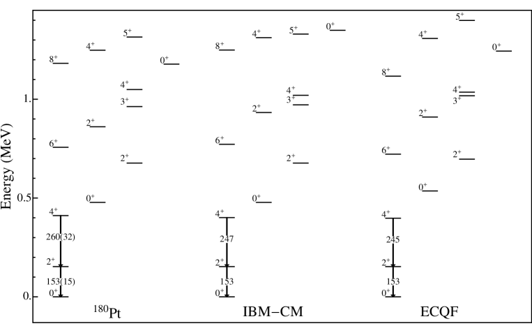
Figure 8: Detailed comparison, including excitation energies and absolute $B(E2)$ values, if known, between experimental data, IBM-CM and ECQF for ¹⁸⁰Pt.

3.3 Comparing the IBM-CM and ECQF: energy spectra and electric quadrupole properties

In the present subsection, we compare the energy spectra as obtained from the IBM-CM and from the ECQF with the experimental energy spectra, for the limited data set (with excitation energy $E_{x}$ less than $\approx$ 1.5 MeV), so as to be able to carry out a detailed comparison between both model calculations, as well as between each of the calculations and the experimental data (see Fig. 4). It becomes clear, by inspecting these results, that both approaches seem equally good in describing the experimental energies up to an excitation energy $E_{x}\approx 1.5$ MeV, although, in general, the IBM-CM calculation provides certain improvements with respect to the ECQF results. A striking result is that the experimental energy spectra in ^178-186Pt are virtually identical, pointing towards a common underlying collective structure.

A more detailed test of the content of the resulting wave functions comes from the $B(E2)$ reduced transition probabilities and from the electric quadrupole moments. The trends for a number of important E2 transitions and for electric quadrupole moments are presented in Figs. 5, 6, and 7. In Fig. 5, we show the absolute $B(E2)$ values for the yrast band. First of all, one observes close similarities between both theoretical approaches and good agreement with the experimental data (we show the two non-overlapping $B(E2;4^{+}_{1}\rightarrow 2^{+}_{1})$ experimental values for ¹⁸⁰Pt). In particular, the increase in the $B(E2)$ values with increasing angular momentum $J$, as well as a saturation near the higher spin $J=8$ value is well reproduced. Moreover, when moving from the lighter isotopes up to the mid-shell region a steady increase in the $B(E2)$ values shows up, followed by a rather smooth decrease when moving towards the heavier Pt isotopes. In Fig. 6, a number of interband $B(E2)$ values are plotted. Here, some clear differences between IBM-CM and ECQF show up, especially for the $B(E2;2^{+}_{2}\rightarrow 0^{+}_{1})$, $B(E2;2^{+}_{2}\rightarrow 2^{+}_{1})$ and $B(E2;3^{+}_{1}\rightarrow 2^{+}_{2})$ values in the lighter Pt isotopes. Progressing towards the heavier isotopes, both approaches provide overall similar results. In comparing with the scarce available experimental data (only known for the heavier Pt isotopes), the agreement is satisfactory. In Fig. 7, the quadrupole moments of some yrast and quasi-$\gamma$ band states are given. In general, both theoretical approaches show the same variation with angular momentum $J$ and mass number $A$. Unfortunately, there exist very few data to test this behavior: experimental quadrupole moments are only known for the heavier ^192,194Pt isotopes [72, 81]. In the lighter isotopes, a negative value of quadrupole moment for the yrast band state results, which is increasing and approaches an almost vanishing value for the heavier Pt isotopes. For the non-yrast $2^{+}_{2}$, a positive quadrupole moment results, which is decreasing in approaching the heavier isotopes. Both theoretical models result again in a similar behavior. For the non-yrast $4^{+}_{2}$ state, the ECQF results in a more smooth variation, changing sign between $A=186$ and $A=188$, as compared with the IBM-CM results. Both descriptions tend towards a much reduced quadrupole moment in the heavier isotopes. The main differences between both approaches is that, in general, the ECQF generates a larger range for the quadrupole moments (larger negative quadrupole moments for the yrast band and $4^{+}_{2}$ state) along the whole chain of isotopes and, the quadrupole moments for the heavier isotopes become zero for the IBM-CM (for all $J$ values) while different from zero but having opposite signs with respect to the experimental data in the ECQF. This effect is a consequence of the differences in the values of $\chi$ that were used in the IBM-CM (with $\chi_{N}$ and $\chi_{N+2}$=0) and ECQF, respectively.

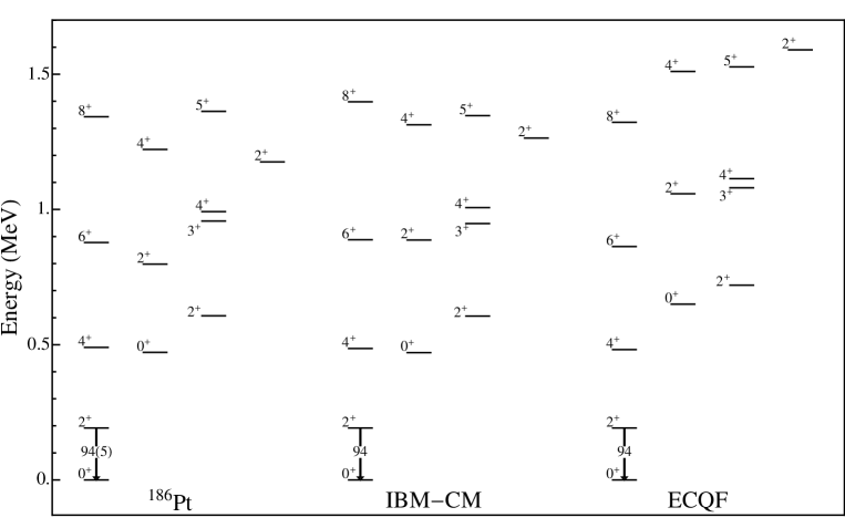
Figure 9: Detailed comparison, including excitation energies and absolute $B(E2)$ values, if known, between experimental data, IBM-CM and ECQF for ¹⁸⁶Pt.

In Tables 5 and 6 and in Tables 7, 8, 9, and 10, in appendix A, we compare the experimental $B(E2)$ values and the electric quadrupole moments with the IBM-CM and ECQF theoretical results, respectively. For the absolute $B(E2)$ values (Table 5) we observe an overall similarity between both approaches and a reasonably good agreement with the experimental data. In the case of ¹⁷⁸Pt, the ECQF $B(E2)$ values along the yrast band are between $15-20\%$ larger compared to the IBM-CM results and the data. In ¹⁸⁰Pt, ¹⁸⁴Pt, ¹⁹²Pt, and ¹⁹⁴Pt both theoretical approaches provide strongly similar values and good agreement with the experimental data. However, in ¹⁹⁴Pt, the $E2$ transitions decaying from the $0^{+}_{2}$ state into the $2^{+}_{1,2}$ states show significant differences between the ECQF and IBM-CM approach, as well as for the $0^{+}_{4}$ to $2^{+}_{1}$ E2 transition. This may point towards a slightly better description of the structure of the excited $0^{+}_{2}$ and $0^{+}_{4}$ states within the IBM-CM description. However, both the ECQF and IBM-CM deviate strongly from the experimental value for the $0^{+}_{4}$ to $2^{+}_{2}$ E2 transition. Thus, it may also turn out that some of the improvements of the IBM-CM over the ECQF could be related to the use of two effective charges instead of one. Experiments to extract E0 transition rates decaying from these $0^{+}$ states are therefore very important. The relative $B(E2)$ values are presented in Tables 7, 8, 9, and 10 in the appendix A in view of the extensive character of that table. There, we give all data used in order to extract these relative values starting from the intensities of $\gamma$-transitions, specifying the decay of specific levels. Regarding the quadrupole moments (Table 6), where experimental data are only available for ^192-194Pt, the IBM-CM predicts a vanishing quadrupole moments for all spin $J$ states. The ECQF predicts finite quadrupole moments but with a sign opposite to the experimental one. The analysis of the data indicates that the ¹⁹⁴Pt nucleus corresponds to an oblate but quite $\gamma$-soft structure  [72]. The IBM-CM predicts these nuclei as $\gamma$-unstable nuclei, while the ECQF describes them as prolate nuclei. These data should allow for an improved description and constrain the parameters in better way.

Isotope	Transition	Experiment	IBM-CM	ECQF
176Pt	$2_{1}^{+}\rightarrow 0_{1}^{+}$	87(8)	87	87
	$4_{1}^{+}\rightarrow 2_{1}^{+}$	163(15)	144	159
	$6_{1}^{+}\rightarrow 4_{1}^{+}$	174(16)	183	199
	$8_{1}^{+}\rightarrow 6_{1}^{+}$	192(25)	192	219
178Pt	$4_{1}^{+}\rightarrow 2_{1}^{+}$	195(18)	195	195
	$6_{1}^{+}\rightarrow 4_{1}^{+}$	186(14)	199	230
	$8_{1}^{+}\rightarrow 6_{1}^{+}$	206(23)	195	246
180Pt	$2_{1}^{+}\rightarrow 0_{1}^{+}$	153(15)	153	153
	$4_{1}^{+}\rightarrow 2_{1}^{+}$	260(32)	247	245
		140(30)
184Pt	$2_{1}^{+}\rightarrow 0_{1}^{+}$	112(5)	112	112
	$4_{1}^{+}\rightarrow 2_{1}^{+}$	210(8)	186	180
	$6_{1}^{+}\rightarrow 4_{1}^{+}$	225(11)	220	212
	$8_{1}^{+}\rightarrow 6_{1}^{+}$	280(30)	235	227
	$10_{1}^{+}\rightarrow 8_{1}^{+}$	300(50)	239	231
186Pt	$2_{1}^{+}\rightarrow 0_{1}^{+}$	94(5)	94	94
188Pt	$2_{1}^{+}\rightarrow 0_{1}^{+}$	82(15)	82	82
190Pt	$2_{1}^{+}\rightarrow 0_{1}^{+}$	56(3)	56	56
192Pt	$2_{1}^{+}\rightarrow 0_{1}^{+}$	57.1(12)	57	57
	$2_{2}^{+}\rightarrow 0_{1}^{+}$	0.54(4)	0.0	0.28
	$2_{2}^{+}\rightarrow 2_{1}^{+}$	109(7)	80	74
	$3_{1}^{+}\rightarrow 4_{1}^{+}$	38(9)	28	28
	$3_{1}^{+}\rightarrow 2_{2}^{+}$	102(10)	64	61
	$3_{1}^{+}\rightarrow 2_{1}^{+}$	0.68(7)	0.0	0.44
	$4_{1}^{+}\rightarrow 2_{1}^{+}$	89(5)	79	79
	$6_{1}^{+}\rightarrow 4_{1}^{+}$	70(30)	90	87
194Pt	$2_{1}^{+}\rightarrow 0_{1}^{+}$	49.2(8)	49.6	49
	$2_{2}^{+}\rightarrow 0_{1}^{+}$	0.29(4)	0.0	0.21
	$2_{2}^{+}\rightarrow 2_{1}^{+}$	89(11)	66	63
	$4_{1}^{+}\rightarrow 2_{1}^{+}$	85(5)	66	67
	$4_{2}^{+}\rightarrow 4_{1}^{+}$	14	32	33
	$4_{2}^{+}\rightarrow 2_{1}^{+}$	0.36(7)	0.0	0.0
	$4_{2}^{+}\rightarrow 2_{2}^{+}$	21(4)	35	37
	$6_{1}^{+}\rightarrow 4_{1}^{+}$	67(21)	67	72
	$0_{2}^{+}\rightarrow 2_{1}^{+}$	0.63(14)	0.91	4.5
	$0_{2}^{+}\rightarrow 2_{2}^{+}$	8.4(19)	9.2	39
	$0_{4}^{+}\rightarrow 2_{1}^{+}$	14.1(12)	14	0.02
	$0_{4}^{+}\rightarrow 2_{2}^{+}$	14.3(14)	0.0	0.0

Table 5: Comparisons of the experimental absolute $B(E2)$ values (given in units of W.u.) with the IBM-CM Hamiltonian and the ECQF results [38]. Data are taken from the Nuclear Data Sheets [47, 48, 49, 50, 51, 52, 53, 54, 55, 56, 57, 58], complemented with references presented in section 2.

Isotope	State	Experiment	IBM-CM	ECQF
192Pt	$2_{1}^{+}$	0.6(2)a	0	-0.327
194Pt	$2_{1}^{+}$	0.409$(^{+62}_{-43})^{b}$	0	-0.288
	$4_{1}^{+}$	0.751$(^{+92}_{-105})^{b}$	0	-0.308
	$6_{1}^{+}$	0.195$(^{+85}_{-188})^{b}$	0	-0.284
	$8_{1}^{+}$	[-0.06,0.28]b	0	-0.26
	$2_{2}^{+}$	-0.303$(^{+93}_{-37})^{b}$	0	0.259
	$4_{2}^{+}$	-0.06(11)b	0	0.09

Table 6: Comparison of the experimental quadrupole moments (given in e$\cdot$b.) with the IBM-CM Hamiltonian and the ECQF results [38]. Data are taken from [81] (a) and [72] (b).

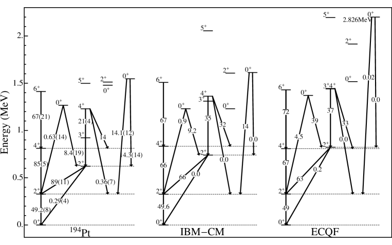
Figure 10: Detailed comparison, including excitation energies and absolute $B(E2)$ values, if known, between experimental data, IBM-CM and ECQF for ¹⁹⁴Pt.

We now present in Figs. 8, 9, and 10 the energy spectra (up to $E_{x}\approx 1.5$ MeV) in order to emphasize differences and similarities between the two theoretical approaches.

In the case of ¹⁸⁰Pt (Fig. 8), the yrast band is well described in both calculations up to the $4^{+}$ level, but slightly high in the IBM-CM while slightly low in the ECQF for the higher-spin members. The $0_{2}^{+}$ band is correctly described in both approaches, although the band head is better reproduced by the IBM-CM. The odd-even staggering is clearly better described by the IBM-CM.

For ¹⁸⁶Pt (see Fig. 9), the yrast band is correctly described in both approaches, IBM-CM and ECQF. The $0_{2}^{+}$ band is rather well described by the IBM-CM calculation even though the spacings in the band are too big compared with the data. Using the ECQF approximation, the $0_{2}^{+}$ band head lies slightly high compared with the experimental position and here too, the energy spacings are too big compared with the data. For the pseudo-$\gamma$ band the situation is quite similar, with a rather good IBM-CM description, i.e., band head, moment of inertia and odd-even staggering. In the ECQF calculation, the band head appears somewhat higher in excitation energy while the moment of inertia is slightly smaller than the experimental one, even though the odd-even staggering is well reproduced.

The comparison for ¹⁹⁴Pt is presented in Fig. 10. Here, we observe a good description of the yrast band, including $B(E2)$ values, for both theoretical approaches. The position of the $0_{2}^{+}$ state is correctly reproduced by both calculations. The description of the pseudo-$\gamma$ band is only qualitatively reproduced by both approaches: the band head comes out too high, the even-odd staggering is incorrect and the moment of inertia is too small. A similar observation results in the description of the $0_{3}^{+}$ band, although, in this case the band-head is better reproduced by the ECQF.

3.4 The intruder structure in the IBM-CM results

Having noticed the strong similarities in both excitation energy and $B(E2)$ reduced transition probabilities considering the particular set of levels up to $\approx$ 1.5 MeV, it is important to study in more detail the particular distribution of the configurations containing $N$ bosons (and thus also those with $N+2$ bosons) as a function of the changing mass (neutron) number passing through the Pt isotopes and for the various $J^{\pi}$ values according to the energy spectra as presented in Fig. 4. In Fig. 11, we present that part of the wave function contained within the N-boson subspace, expressed by the weight $w^{k}(J,N)$, of the two lowest-lying states $(k=1,2)$ for a given angular momentum.

Figure 11: The regular configuration content, expressed by the weight $w^{k}(J,N)$ (see text), for the two lowest-lying states $(k=1,2)$ for each $J$ value (full lines with closed symbols correspond with the first state while dashed lines with open symbols correspond with the second state) resulting from the IBM-CM calculation, as presented in Fig. 4.

The results obtained for the angular momentum $0^{+},2^{+},3^{+},4^{+}$ states (left-hand part) retain the major structure also observed in the calculations carried out by Harder et al. [42] and also shown in the left-hand part of Fig. 3, although now no longer symmetric with respect to the mid-shell point. The variation in the weight of the N-boson content also exhibits a far more complex structure between neutron (mass) number $N=110$ $(A=188)$ and $N=116$ $(A=194)$. This fact is due to the specific values for the parameters characterizing the IBM-CM Hamiltonian for these isotopes. One notices a sudden increase in the N-boson weight of the wave functions. For the higher-spin values $5^{+},6^{+},7^{+},8^{+}$, the right-hand part of Fig. 11 shows serious differences when comparing to the right-hand part of Fig. 3, in particular, for the second excited state of each of the spin values shown. Just like for the left-hand part of the Fig. 11, a rather complex structure results when passing in between neutron (mass) number $N=110$ $(A=188)$ and $N=116$ $(A=194)$.

In order to study more clearly the effects on the energy spectra, induced by the mixing term, we recalculate the spectra using the Hamiltonian parameters shown in Table 3, but now switching off the mixing term. The spectra are presented in Fig. 12 where we show the two lowest regular and the lowest intruder state for different angular momentum values. Here, we observe a rather flat behavior of the energy for the regular states. The energy of the intruder states is smoothly decreasing until the neutron mid-shell value at $N=104$, where it starts increasing again. This effect results mainly from the smooth change of the Hamiltonian parameters when passing from isotope to isotope.

A simultaneous analysis of Figs. 11 and 12, combined with the rules of a simple two-level mixing model, allows us to explain the sudden increase of the regular component for all $J^{\pi}$ values at $A=188$. In Fig. 12, the unperturbed energies, i.e., excluding the mixing term, are plotted. Here, one observes the close approach of pairs of regular and intruder states with a given angular momentum, especially in the region around $A=188$. The mixing term, coupling the regular ($N$) and intruder ($N+2$) configurations, can now result in the interchange of character between the states and therefore in the sudden increase of the regular component content of the wave function. For states with $J>4$, the effect is even more dramatic because the unperturbed energy of the intruder configuration always lies below the unperturbed energy of the regular one and as a consequence, the interchange in character with the regular configuration at the point of closest approach is enhanced. Eventually, moving towards $A=194$, the unperturbed energies of the intruder configurations are moving up and cross the energies of the regular configurations. Therefore, as shown in Fig. 11, from $A=194$ onwards, the two lowest-lying states for each $J^{\pi}$ value have become regular (N-component, mainly) states.

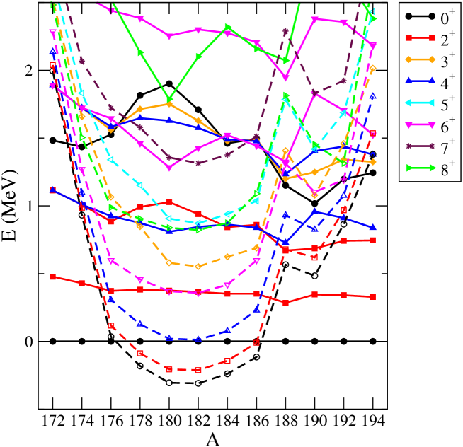
Figure 12: Energy spectra for the IBM-CM Hamiltonian presented in Table 3, switching off the mixing term. The two lowest-lying regular states and the lowest-lying intruder state for each of the angular momenta are shown (full lines with closed symbols for the regular states while dashed lines with open symbols are used for the intruder states).

Figure 13: Comparison of the energy spectra for the IBM-CM and ECQF for ¹⁸⁴Pt up to an excitation energy of $E_{x}\approx 5$ MeV.

4 Similarities and differences between the two model spaces

As was already noticed in the calculations carried out by Harder et al. [42] and in the calculations presented in section 3.2, there are a number of properties in the Pt nuclei, such as excitation energies and $B(E2)$ values for the set of levels below $\approx$ 1.5 MeV, that do not seem to be very sensitive to the use of a smaller model space as compared to the use of a much larger model space incorporating both regular and particle-hole excited intruder configurations, explicitly. This can partly be expected because precisely those observables - excitation energies, $B(E2;2^{+}_{1}\rightarrow 0^{+}_{1})$, $B(E2;2^{+}_{2}\rightarrow 0^{+}_{1})$, and $B(E2;2^{+}_{2}\rightarrow 2^{+}_{1})$ - when experimentally known, were used in the fitting procedure in both the IBM-CM and the ECQF calculations.

4.1 The energy spectra at high excitation energy: comparing the IBM-CM and ECQF

When comparing the IBM-CM calculations (which is using a model space that contains both, $N$ boson and $N+2$ boson configurations) with the ECQF calculations (which is using a model space with N bosons only), it is unavoidable that moving up in excitation energy, at some point, clear-cut differences in the density of states with given $J^{\pi}$ value should show up (the full dimension in the IBM-CM more than doubles the one of the ECQF). It is interesting to make the comparison between both. In Fig. 13, we illustrate this in the specific case of ¹⁸⁴Pt (which is typical for all nearby nuclei), which is situated in a region where a number of unperturbed configurations containing $N$ and $N+2$ bosons, respectively, appear at about the same unperturbed energy and thus start a complex crossing pattern in the IBM-CM approach. In Fig. 13, one observes that up to an excitation energy of about $2$ MeV, there are no obvious differences between the IBM-CM and the ECQF theoretical results. Above this energy, different patterns are showing up. In particular in the IBM-CM one observes a rather smooth distribution of levels, while in the ECQF the energy levels appear more separated in blocks spaced by about $0.5$ MeV. This separation in blocks accentuates when increasing the value of the angular momentum. This turns out to be an indication that one is running out of model space if one restricts to $[N]$ configurations only.

4.2 Eliminating the N+2 configurations: a mapping procedure

We point out that the very close resemblance of a part of the energy spectrum (restricting to excitation energies below $\approx$ 1.5 MeV) and corresponding $B(E2)$ values, can most probably be understood from a mapping of the larger model space, used in the IBM-CM in which configurations with both $N$ and $N+2$ components are considered, onto the smaller space, used in the ECQF formulation, in which only the $N$ boson configurations are kept. Thereby, an effective Hamiltonian acting in the smaller space is defined through the mapping of the lowest energy eigenvalues and similarly for the corresponding model transition operators. We can describe the wave functions in the IBM-CM as follows

$$\Psi(k,JM) = \sum_{i}a^{k}_{i}(J;N)\psi((sd)^{N}_{i};JM)$$ (11)

$$+ \ \sum_{j}b^{k}_{j}(J;N+2)\psi((sd)^{N+2}_{j};JM)~{}.$$

We can also consider a limited number of basis states, i.e., only the components with $N$ bosons. This basis spans the smaller model space and the corresponding model wave function can be expressed as

$$\Psi^{\prime}(k,JM)=\sum_{l}a^{\prime k}_{l}(J;N)\psi((sd)^{N}_{l};JM\rangle~{},$$ (12)

i.e., that part of the “true” wave function that lies within the small model space. If we then require that the lowest energy eigenvalues $E_{k}(JM)$, for the large space, be reproduced exactly within the much smaller model space, one can determine an effective Hamiltonian acting in the reduced model space containing only configurations with N bosons by a mapping procedure

$$\langle\Psi^{\prime}(k,JM)\mid\hat{H}^{eff.}\mid\Psi^{\prime}(k,JM)\rangle=E(k,JM)~{}.$$ (13)

Using the projection operator $\hat{\bf P}=\sum_{i\subset N}\mid(sd)^{N}_{i};JM\rangle\langle(sd)^{N}_{i};JM\mid$, which projects onto the model space containing only N-boson configurations and the operator $\hat{\bf Q}=\sum_{j\subset{N+2}}\mid(sd)^{N+2}_{j};JM\rangle\langle(sd)^{N+2}_{j};JM\mid$, projecting onto the N+2-boson model configurations, an effective Hamiltonian acting in the reduced model space can be constructed [82] as

$$\hat{H}^{eff.}=\hat{H}+\hat{H}\frac{\hat{\bf Q}}{E(k,JM)-\hat{H}^{0}}\hat{H}+....$$ (14)

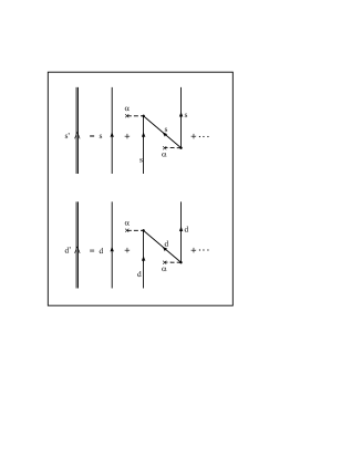
Figure 14: Schematic diagram representing the effect of eliminating the N+2 space on the single particle boson energies.

Although this formal procedure cannot easily be carried out starting from the Hamiltonian used in the IBM-CM model space to construct the effective Hamiltonian acting in the reduced model space with N bosons only, it seems possible to show numerically that the procedure will work. Indeed, the low-lying levels calculated in the IBM-CM model space up to $E_{x}\approx 1.5$ MeV match up very well with the corresponding levels using the ECQF calculation within the N-boson model space, only. Considering the lowest-order diagrams that follow from the expansion in Eq. (14), it can easily be seen that eliminating the N+2 components implies changes in both the boson single-particle energies $\varepsilon_{s}$ and $\varepsilon_{d}$ (see Fig. 14), as well as in the parameters $\kappa$, $\kappa^{\prime}$, and $\chi$ appearing in the interaction part of the Hamiltonian. Work is in progress to try to carry out the mapping for the most simple terms appearing in the IBM-CM Hamiltonian.

4.3 Observables and sensitivity to the enlarged model space

The idea of comparing truncated model spaces with much larger model spaces and the fact that a number of observables obtained in these model spaces might still turn out to be very similar when comparing to experimental data was illustrated a long time ago by Cohen, Lawson and Soper [83, 84]. By theoretically constructing a set of nuclei, called the Pseudonium nuclei ^40-48Ps, starting from a model space consisting of two degenerate $1d_{3/2}$ and $1f_{7/2}$ single-particle orbitals, containing between 4 and 12 neutrons and a given two-body interaction (a Yukawa force was used), they showed that these energy spectra interpreted as pseudo-data, could be fitted very well using a much restricted model space consisting of the $1f_{7/2}$ orbital only, now containing between 0 and 8 neutrons. It turned out that the effective interaction matrix elements, fitted to the Pseudonium nuclei, was corresponding to quite a different interaction than the force used at first in the larger model space. They moreover showed that other observables, such as $B(E2)$ values for the strongest transitions, were very similar even though the wave functions were very different. A different set of Pseudonium nuclei were constructed making use of a model space consisting of two degenerate $1p_{1/2}$ and $1d_{3/2}$ single-particle states that could contain both protons and neutrons, up to maximally 12 nucleons. Very much the same conclusion resulted when analyzing corresponding states using a model space consisting of the $1d_{3/2}$ orbital only [85]. In the latter study, it was pointed out that quadrupole moments seemed to be a better observable to probe differences, with particularly chosen transfer reactions, becoming highly sensitive to the use of different model spaces. It shows that a number of observables (excitation energies, $B(E2)$,…) are very insensitive to configuration mixing arising from the excitation of zero-coupled pairs out of the closed shell. This may turn out to be the same underlying mechanism in our present IBM-CM study.

This study of the actual wave function content and the way to test it has, more recently, been explored, e.g., in the study of the nucleus ⁴⁰Ca [86]. It turns out that the $0^{+}$ ground state only consists of 65% closed sd shell (or 0p-0h) and exhibits 29% of 2p-2h excitations out of the $2s_{1/2},1d_{3/2}$ normally filled orbitals into the $1f_{7/2},2p_{3/2},1f_{5/2},2p_{1/2}$ higher-lying orbitals, even containing up to 5% of 4p-4h excitations. This large model space is effectively needed in order to describe the higher-lying strongly deformed bands and superdeformation as experimentally observed in ⁴⁰Ca. A study of isotopic shifts in the even-even Ca nuclei, moving from $A=40$ to $A=48$ could be reproduced well by including explicitly, mp-nh excitations across the $Z=20$, $N=20$ ”closed” shell, using a slightly smaller model space than the one used before [87]. This points out that one can indeed find observables that are sensitive to the important components of the wave function and thus be able to discriminate between various approaches that give quite similar results when restricting to a subset of data, only.

Therefore, in a forthcoming paper, we shall compare the results of both, the IBM-CM and ECQF calculations with a data set that encompasses besides excitation energies and $B(E2)$ values also quadrupole moments, $g(2_{1}^{+})$ values, $\alpha$-decay hindrance factors, isotopic shifts, $\rho^{2}$ values extracted from E0 transitions, as well as results derived from properties characterizing the energy spectra and E0 transitions in the adjacent odd-mass nuclei. Transfer reactions are most probably one of the best tests to explore the detailed composition of the nuclear wave function. They have been shown to be able to detect the presence of core-excited configurations in different mass regions. Such a comparison should allow to compare the nuclear wavefunctions derived in the smaller N space with the wavefunctions containing both N and N+2 configurations (inclusion of particle-hole excitations, explicitly).

5 Conclusions

In the present study, we have analyzed certain aspects related to the role of intruder excitations in the Pt isotopes. To start with, we have presented the experimental knowledge in this mass region on energy spectra and absolute $B(E2)$ values, however restricting to an excitation energy up to $1.5$ MeV. Next, we have performed a set of IBM-CM calculations for the isotopes ^172-194Pt and compared them with previous ECQF calculations, noticing that for the subset of states below $\approx 1.5$ MeV, both descriptions are roughly comparable. However, if one extends both calculations up to 5 MeV, differences in the distribution of the theoretical levels start to show up. We have suggested that the similarities between both model spaces can be explained through an appropriate mapping with a low-energy cut-off in the excitation energy of $\approx 1.5$ MeV. This mapping may shed light on the way to extract the parameters that appear in the smaller model space (which amounts to four in the ECQF study) starting from the larger model space, containing in the present IBM-CM approach eight free parameters. We have also made reference to earlier studies by Cohen, Lawson and Soper, carried out within the context of the nuclear shell-model, where it was shown that calculated energy spectra and other observables, using a given model space and two-body interaction in the case of strong mixing, can be fitted very well using a restricted model space and an effective or renormalized interaction. They showed the insensitivity of a number of observables (such as excitation energies and $B(E2)$ values) to strong configuration mixing arising from the excitation of $0^{+}$ coupled pairs out of a closed shell. These studies stressed the need to detect (i) all states (complete spectroscopy) as well as, (ii) the importance to study specific observables in order to probe the nuclear wavefunction in greater detail.

The fact that for the neutron-deficient Pb and Hg nuclei, a fit using the smaller model space cannot be obtained (in particular the low-lying $0^{+}_{2}$ energies) [38] is particularly relevant in this respect. It shows that in the case of weak mixing between the regular low-lying configurations (N-space) and particle-hole (p-h) pair excitations across $Z=82$ closed shell (N+2,… space), the intruder states are clearly visible and exhibit a distinct energy systematics. This points out the need to consider a model space containing both regular and p-h pair configurations. However, in situations where the p-h pair excitations appear at nearly the same unperturbed energy as the regular excitations and strong mixing follows, the observed excitation energies do not show any more such a distinct separation. Still, the excitation energies and electric quadrupole properties for states below $E_{x}\approx$ 1.5 MeV are very similar using the larger and the smaller model space, excluding p-h degrees of freedom, explicitely (section 3.3 and section 3.4). This is a most interesting result, in view of the highly-different wave functions that enter the calculations and may be understood constructing the mapping referred to before. Moreover, the arguments put forward in the study of the Pseudonium nuclei by Cohen, Lawson and Soper of concealed configuration mixing of $0^{+}$ coupled pairs, are interesting in the prospect of accomplishing a mapping. Work is in progress on this important issue. Moreover, in a forthcoming paper, we shall present the results of a comparison covering an as complete as possible data set (encompassing also, e.g., $\alpha$-decay hindrance factors, $g(2^{+}_{1})$ factors, isotopic shifts, E0 decay properties, as well as properties in the spectra of neighboring odd-mass Pt and Au nuclei) with the two theoretical approaches, i.e., considering a reduced model space versus a larger model space including particle-hole excitations explicitly, within the Interacting Boson Model context. Transfer reactions may prove to be very effective in showing the detailed structure of the nuclear wave functions.

6 Acknowledgment

We thank M. Huyse, P.Van Duppen, and P.Van Isacker for continuous interest in this research topic and J.L. Wood for stimulating discussions in various stages of this work. Financial support from the “FWO-Vlaanderen” (KH and JEGR) is acknowledged. This research was also performed in the framework of the BriX network (IAP P6/23) funded by the ’InterUniversity Attraction Poles Programme - Belgian State-Belgian Science Policy’. This work has also been partially supported by the Spanish Ministerio de Ciencia e Innovación and by the European regional development fund (FEDER) under projects number FPA2006-13807-C02-02 and FPA2007-63074, by Junta de Andalucía under projects FQM318, and P07-FQM-02962 and by the Spanish Consolider-Ingenio 2010 Programme CPAN (CSD2007-00042).

Appendix A Appendix: Relative $B(E2)$ values in ^180-194Pt

Since the number of absolute $B(E2)$ values known in the ^180-194Pt nuclei is quite restricted, we also cover relative $B(E2)$ values. Extracting those relative values, one needs detailed information on the $\gamma$-ray intensities for the transitions originating from a given initial state. In order to do so, we have made use of the adopted values given in the most recent volume of the Nuclear Data Sheets (NDS), covering the mass range from $A=180$ up to $A=194$ and are taken from [51] ($A=180$), [54] ($A=186$), [55] ($A=188$), [56] ($A=190$), [57] ($A=192$) and [58] ($A=194$). In a number of cases, i.e., when the latest issue of NDS was published more than 10 years ago, we have taken data from recent literature. This was the case for $A=182$ ([52] dates from 1995), in which case the necessary data were taken from a study of Davidson et al. [66] and also for $A=184$ with the NDS dating to 1989 [53]. In the latter case, we have used the update on ¹⁸⁴Pt, kindly supplied by Baglin [79], information which will soon be published in a forthcoming issue of NDS. For $A=192$, we have, for the transitions decaying from the $2^{+}_{3}$ level, taken the data from McCutchan et.al. [71].

We have taken from these data the transition energies, intensities and corresponding errors. In the table that follows, we also give the evaluated information on multipolarities in situations where one can expect that besides $E2$ transitions, $M1$ transitions and, in situations where $J_{i}=J_{f}$, also $E0$ transitions can contribute. Thereby we follow the conventions used by the evaluators of NDS: (…) stands for very strong indications for the multipolarities given between parenthesis, [ ] stands for multipolarities deduced from information on the decay scheme, even compelling, but not measured, (Q) or Q stands for a transitions with quadrupole multipolarity, but no unambigous parity information known. In a number of cases, $\delta(E2/M1)$ mixing ratios have been measured and are given. In a number of transitions that have been taken as a reference transition to derive the relative $B(E2)$ values, but might contain $M1$ admixtures, we explicitely mention if a mixing ratio is know. In a number of situations such as the $2^{+}_{2}\rightarrow 2^{+}_{1}$ transition, the $E2$ assignment in NDS, even with the mixing ratio unknown, is made on the basis of measured conversion coefficients, excluding important $M1$ admixtures. For all nuclei considered here, we have assumed this particular transition to be $E2$, so the numbers deduced from that may carry a given “uncertainty” with them. Something quite similar occurs for the $3^{+}_{1}\rightarrow 2_{2}$ transition, which has (if present) been taken as the reference transition when deriving relative $B(E2)$ values. In a number of cases, the mixing ratio helps substantially in deciding to fix a reference transition in order to derive relative $B(E2)$ values.

Using the criteria discussed before, we have extracted the experimental relative $B(E2)$ values (with error). The expression used is given by

$$\mbox{B(E2)}=100\times\left(\frac{\mbox{I}_{\gamma}}{\mbox{I}_{\gamma}^{ref}}\right)\times\left(\frac{\mbox{E}_{\gamma}^{ref}}{\mbox{E}_{\gamma}}\right)^{5}\times\left(\frac{1+\frac{1}{\delta^{2}_{ref}}}{1+\frac{1}{\delta^{2}}}\right),$$ (15)

where ref stands for the reference transition.

The related errors are given by the expression

$$\Delta(\mbox{B(E2)})=\mbox{B(E2)}$$

$$\times\sqrt{\ \left(\frac{\Delta(\mbox{I}_{\gamma})}{\mbox{I}_{\gamma}}\right)^{2}+\left(\frac{\Delta(\mbox{I}_{\gamma}^{ref})}{\mbox{I}_{\gamma}^{ref}}\right)^{2}+4\left(\frac{\Delta(\delta)}{\delta}\right)^{2}+4\left(\frac{\Delta(\delta_{ref})}{\delta_{ref}}\right)^{2}},$$ (16)

where $\Delta()$ stands for the absolute error.

Here, the relative errors for both the reference transition, the one that is taken as the relative transition, as well as the relative errors on mixing ratios (again for the reference transition and the one that is taken as the relative transition), if the latter are available, have to be taken into account in a quadratic way. Note that we did not include the contribution from the error of the gamma energies because they are negligible.

	Transition	Eγ	Iγ	Mult.	$\delta$	Exp.	IBM-CM	ECQF
		(keV)
180Pt	$2_{2}^{+}\rightarrow 0_{2}^{+}$	199	5(2)			630(250)	84	120
	$2_{2}^{+}\rightarrow 4_{1}^{+}$	207	0.9(5)			26(15)	13	20
	$2_{2}^{+}\rightarrow 2_{1}^{+}$	524	100(2)	E0+E2	$<$-11	100	100	100
	$2_{2}^{+}\rightarrow 0_{1}^{+}$	678	35(3)			9.7(9)	4.5	6
	$2_{3}^{+}\rightarrow 2_{2}^{+}$	184	1.1(6)			$<$304	158	158
	$2_{3}^{+}\rightarrow 0_{2}^{+}$	383	14(2)			100	100	100
	$2_{3}^{+}\rightarrow 4_{1}^{+}$	451	18(2)			57(10)	44	50
	$2_{3}^{+}\rightarrow 2_{1}^{+}$	708	15(2)	E0+M1+E2	2.0${}^{+3.6}_{-1.1}$	4.0${}^{+1.7}_{-2.2}$	3.2	0.5
	$2_{3}^{+}\rightarrow 0_{1}^{+}$	861	100(2)			12.4(1.8)	13	10
	$3_{1}^{+}\rightarrow 2_{2}^{+}$	286	3.5(7)	∗	Unknown	100	100	100
	$3_{1}^{+}\rightarrow 4_{1}^{+}$	552	13(2)			$<$14	17	17
	$3_{1}^{+}\rightarrow 2_{1}^{+}$	889	100(2)	E2	$<$-13	16(3)	11	9
	$4_{2}^{+}\rightarrow 2_{2}^{+}$	372	15(4)			100	100	100
	$4_{2}^{+}\rightarrow 4_{1}^{+}$	639	100(13)			45(13)	35	25
	$4_{2}^{+}\rightarrow 2_{1}^{+}$	896	17(8)			1.4(8)	0.1	0.2
	$0_{3}^{+}\rightarrow 2_{2}^{+}$	500	13(8)			100	100	100
	$0_{3}^{+}\rightarrow 2_{1}^{+}$	1024	100(10)			21(13)	1.4	0.33
	$4_{3}^{+}\rightarrow 2_{3}^{+}$	387	70(40)			100	100	100
	$4_{3}^{+}\rightarrow 2_{2}^{+}$	572	$\approx$ 21			$\approx$4	5.1	0.5
	$4_{3}^{+}\rightarrow 4_{1}^{+}$	837	27(7)			$<$0.8	0.8	0.7
	$4_{3}^{+}\rightarrow 2_{1}^{+}$	1095	100(20)			0.8(5)	4.1	0.9
	$5_{1}^{+}\rightarrow 3_{1}^{+}$	353	19(5)			100	100	100
	$5_{1}^{+}\rightarrow 4_{1}^{+}$	905	100(9)	(M1+E2)		$<$5	4.6	3.3
182Pt	$2_{2}^{+}\rightarrow 2_{1}^{+}$	512	23.3(26)	E0+(M1)+E2∗	Unknown	100	100	100
	$2_{2}^{+}\rightarrow 0_{1}^{+}$	667	8.0(10)			9.2(15)	12	6.4
	$2_{3}^{+}\rightarrow 0_{2}^{+}$	356	2.6(7)			100	100	100
	$2_{3}^{+}\rightarrow 4_{1}^{+}$	436	3.4(3)			47(13)	25	49
	$2_{3}^{+}\rightarrow 2_{1}^{+}$	701	1.3(3)	E0+M1+E2	0.7${}^{+1.0}_{-0.3}$	0.6${}^{+1.2}_{-0.4}$	2.8	0.7
	$2_{3}^{+}\rightarrow 0_{1}^{+}$	855	15.0(5)			7.2(19)	3.2	5.3
	$3_{1}^{+}\rightarrow 4_{1}^{+}$	523	2.5(3)	[M1,E2]		$<$146	156	189
	$3_{1}^{+}\rightarrow 2_{1}^{+}$	787	13.7(19)	(M1+E2)	$>$5	100	100	100

Table 7: Comparisons of the experimental relative $B(E2)$ values with the IBM-CM Hamiltonian and the ECQF results [38]. ¿From left to right we give: isotope, transition, $\gamma$-ray energy, intensity of the transition, multipolarity, $\delta$ value, experimental relative $B(E2)$ value, IBM-CM calculation and ECQF calculation. Data are taken from [51, 54, 55, 56, 57, 58], C. Baglin [79], complemented with references [66, 71].
^∗ Pure E2 transition assumed.

	Transition	Eγ	Iγ	Mult.	$\delta$	Exp.	IBM-CM	ECQF
		(keV)
184Pt	$2_{2}^{+}\rightarrow 2_{1}^{+}$	486	100(10)	(E0)+E2+M1∗	Unknown	100	100	100
	$2_{2}^{+}\rightarrow 0_{1}^{+}$	649	50(8)			61(21)	83	87
	$2_{3}^{+}\rightarrow 2_{2}^{+}$	195	2.6(8)	(E0)+M1+E2		$<$415	122	110
	$2_{3}^{+}\rightarrow 0_{2}^{+}$	352	12.0(18)	[E2]		100	100	100
	$2_{3}^{+}\rightarrow 4_{1}^{+}$	408	12.7(19)			51 (11)	55	48
	$2_{3}^{+}\rightarrow 2_{1}^{+}$	681	13.1(20)	E0+M1+E2	-1.2${}^{+0.5}_{-3.5}$	[1.0,4.9]	0.8	0.3
	$2_{3}^{+}\rightarrow 0_{1}^{+}$	844	100(15)			10.5 (22)	10.3	3.6
	$3_{1}^{+}\rightarrow 2_{2}^{+}$	291	3.6(11)	∗	Unknown	100	100	100
	$3_{1}^{+}\rightarrow 4_{1}^{+}$	504	15.7(25)			$<$28	16	18
	$3_{1}^{+}\rightarrow 2_{1}^{+}$	777	100(10)	(M1)+E2	$>$4	19(1)	10	7.9
	$2_{4}^{+}\rightarrow 2_{2}^{+}$	524	8.5(26)	E0+M1+E2∗	Unknown	100	100	100
	$2_{4}^{+}\rightarrow 0_{2}^{+}$	681	12(3)			38(15)	0.8	59
	$2_{4}^{+}\rightarrow 0_{1}^{+}$	1172	22(7)			4.6 (20)	0.1	2.1
	$4_{2}^{+}\rightarrow 2_{2}^{+}$	379	39(6)			100	100	100
	$4_{2}^{+}\rightarrow 4_{1}^{+}$	592	100(14)	(E0)+M1+E2	$\leq$-1.2	21(5)	35	30
	$4_{3}^{+}\rightarrow 3_{1}^{+}$	294	7.7(23)			$<$62	104	30
	$4_{3}^{+}\rightarrow 2_{3}^{+}$	390	51(7)			100	100	100
	$4_{3}^{+}\rightarrow 2_{2}^{+}$	586	18(6)			4.6 (17)	8.7	0.3
	$4_{3}^{+}\rightarrow 4_{1}^{+}$	798	74(12)	E0+M1+E2	1.1(3)	2.2 (1.3)	0.4	0.5
	$4_{3}^{+}\rightarrow 2_{1}^{+}$	1071	100(14)			1.26 (25)	2.7	0.7
	$3_{2}^{+}\rightarrow 2_{4}^{+}$	297	29(8)	∗	Unknown	100	100	100
	$3_{2}^{+}\rightarrow 3_{1}^{+}$	530	$<$1.4	E0+M1+E2		$<$0.27	0	0
	$3_{2}^{+}\rightarrow 2_{3}^{+}$	626	24(7)			$<$2.0	0.03	1.7
	$3_{2}^{+}\rightarrow 2_{2}^{+}$	821	44(13)			$<$0.9	0.4	0.6
	$3_{2}^{+}\rightarrow 4_{1}^{+}$	1034	60(18)			$<$ 0.40	0.02	0.08
	$3_{2}^{+}\rightarrow 2_{1}^{+}$	1307	100(15)			$<$ 0.21	0.03	0.04

Table 8: See caption of Table 7.

	Transition	Eγ	Iγ	Mult.	$\delta$	Exp.	IBM-CM	ECQF
		(keV)
186Pt	$2_{2}^{+}\rightarrow 2_{1}^{+}$	416	100(4)	M1+E2	19${}^{+20}_{-8}$	100	100	100
	$2_{2}^{+}\rightarrow 0_{1}^{+}$	607	62(15)			9.4(23)	5	6.3
	$2_{3}^{+}\rightarrow 4_{1}^{+}$	308	7.7(6)			69(8)	38	39
	$2_{3}^{+}\rightarrow 0_{2}^{+}$	327	15.1(12)			100	100	100
	$2_{3}^{+}\rightarrow 0_{1}^{+}$	799	100(12)			7.6(11)	3.8	2.2
	$3_{1}^{+}\rightarrow 2_{2}^{+}$	349	12.4(8)	M1+E2	2.8(3)	100	100	100
	$3_{1}^{+}\rightarrow 4_{1}^{+}$	466	12.4(6)	(M1+E2)	0.42(7)	4.0(16)	24	19
					3.8(9)	25(13)	24	19
	$3_{1}^{+}\rightarrow 2_{1}^{+}$	765	100(5)	M1+E2	16${}^{+4}_{-3}$	18(4)	9.0	6.7
	$4_{2}^{+}\rightarrow 2_{2}^{+}$	384	63(5)			100	100	100
	$4_{2}^{+}\rightarrow 4_{1}^{+}$	501	100(16)	M1+E2	-0.85(9)	18(5)	37	39
	$4_{2}^{+}\rightarrow 2_{1}^{+}$	800	79(16)			3.2(7)	0.4	0.3
	$2_{4}^{+}\rightarrow 0_{2}^{+}$	704	43(5)			100	100	100
	$2_{4}^{+}\rightarrow 2_{1}^{+}$	985	100(10)	M1+E2	-0.12(6)	0.6(6)	41	49
				M1+E2	3.2(8)	40(21)	41	49
	$2_{4}^{+}\rightarrow 0_{1}^{+}$	1176	48(5)			8.6(13)	3.5	2.4
	$4_{3}^{+}\rightarrow 3_{1}^{+}$	266	19.1(18)			$<$440	115	25
	$4_{3}^{+}\rightarrow 2_{3}^{+}$	424	45(5)			100	100	100
	$4_{3}^{+}\rightarrow 4_{1}^{+}$	732	82(5)	E0+M1+E2		$<$12	2.3	0.3
	$4_{3}^{+}\rightarrow 2_{1}^{+}$	1031	100(5)			2.6(3)	1.4	0.6
	$5_{1}^{+}\rightarrow 3_{1}^{+}$	406	22(7)			100	100	100
	$5_{1}^{+}\rightarrow 4_{1}^{+}$	872	100(7)			$<$10	4.1	3.3

Table 9: See caption of Table 7.

	Transition	Eγ	Iγ	Mult.	$\delta$	Exp.	IBM-CM	ECQF
		(keV)
188Pt	$2_{2}^{+}\rightarrow 2_{1}^{+}$	340	100(4)	E2∗	Unknown	100	100	100
	$2_{2}^{+}\rightarrow 0_{1}^{+}$	605	66(3)			3.7(2)	0.5	2.2
	$0_{2}^{+}\rightarrow 2_{2}^{+}$	193	2.9(7)			100	100	100
	$0_{2}^{+}\rightarrow 2_{1}^{+}$	533	100(4)			21(5)	17	53
	$3_{1}^{+}\rightarrow 2_{2}^{+}$	331	63(3)	E2∗	Unknown	100	100	100
	$3_{1}^{+}\rightarrow 2_{1}^{+}$	671	100(4)			$<$5	0.84	3.3
	$4_{2}^{+}\rightarrow 4_{1}^{+}$	415	45(4)	M1+(E2)		$<$92	83	69
	$4_{2}^{+}\rightarrow 2_{2}^{+}$	479	100(7)			100	100	100
	$4_{2}^{+}\rightarrow 2_{1}^{+}$	820	21(2)	(Q)		1.43(17)	0.4	0.14
	$2_{3}^{+}\rightarrow 0_{2}^{+}$	316	19(2)			100	100	100
	$2_{3}^{+}\rightarrow 4_{1}^{+}$	444	22(2)			21(3)	17	24
	$2_{3}^{+}\rightarrow 2_{1}^{+}$	849	14(5)	E0+M1+E2		$<$0.5	0.3	0.07
	$2_{3}^{+}\rightarrow 0_{1}^{+}$	1115	100(4)			1.0(1)	0.1	0.8
	$2_{4}^{+}\rightarrow 2_{3}^{+}$	198	7.1(24)	∗	Unknown	100	100	100
	$2_{4}^{+}\rightarrow 3_{1}^{+}$	376	17(3)	M1+E2	1.3(3)	6(4)	39	1240
	$2_{4}^{+}\rightarrow 4_{1}^{+}$	642	22(4)			0.9(3)	0.01	1.3
	$2_{4}^{+}\rightarrow 2_{2}^{+}$	707	31(4)	E0+M1+E2		$<$0.8	0.3	16
	$2_{4}^{+}\rightarrow 2_{1}^{+}$	1047	65(7)	E0+M1+E2		$<$0.2	0.05	0.7
	$2_{4}^{+}\rightarrow 0_{1}^{+}$	1313	100(7)			0.11(4)	0.0	0.0
190Pt	$2_{2}^{+}\rightarrow 2_{1}^{+}$	302	100(3)	E2∗	Unknown	100	100	100
	$2_{2}^{+}\rightarrow 0_{1}^{+}$	598	40(3)			1.3(1)	0	1.0
	$3_{1}^{+}\rightarrow 4_{1}^{+}$	180	3.1(3)	M1+E2	3${}^{+2}_{-1}$	49${}^{+9}_{-10}$	43	36
	$3_{1}^{+}\rightarrow 2_{2}^{+}$	319	100(5)	E2∗	Unknown	100	100	100
	$3_{1}^{+}\rightarrow 2_{1}^{+}$	621	56(5)	M1+E2	1.0${}^{+2.0}_{-0.6}$	1.0${}^{+0.6}_{-0.7}$	0	1.7
	$0_{2}^{+}\rightarrow 2_{2}^{+}$	323	35(2)			100	100	100
	$0_{2}^{+}\rightarrow 2_{1}^{+}$	625	100(5)			10.5(8)	10	48
	$4_{2}^{+}\rightarrow 4_{1}^{+}$	391	30(3)	[M1,E2]		$<$140	100	79
	$4_{2}^{+}\rightarrow 2_{2}^{+}$	531	100(8)			100	100	100
	$2_{3}^{+}\rightarrow 0_{2}^{+}$	282	51(4)			100	100	100
	$2_{3}^{+}\rightarrow 3_{1}^{+}$	286	26(2)	(M1)+E2	$>$5	47(1)	0	21
	$2_{3}^{+}\rightarrow 4_{1}^{+}$	466	32(2)			5.1(5)	75	18
	$2_{3}^{+}\rightarrow 2_{2}^{+}$	605	100(2)	M1+(E2)	$<$0.4	$<$0.6	12	9.3
	$2_{3}^{+}\rightarrow 2_{1}^{+}$	907	97(2)	E0+(M1,E2)		$<$0.6	0	0.03
	$2_{3}^{+}\rightarrow 0_{1}^{+}$	1203	14(2)			0.019(3)	0.04	0.6
192Pt	$2_{3}^{+}\rightarrow 4_{1}^{+}$	655	3.3(4)			0.85(11)	64	16
	$2_{3}^{+}\rightarrow 0_{2}^{+}$	244	2.8(3)			100	100	100
	$2_{3}^{+}\rightarrow 3_{1}^{+}$	518	26.8(35)			$<$22	0	18
	$2_{3}^{+}\rightarrow 2_{2}^{+}$	827	3.4(3)			$<$0.3	9	8.4
	$2_{3}^{+}\rightarrow 2_{1}^{+}$	1123	100(4)			$<$1.7	0	0.02
	$2_{3}^{+}\rightarrow 0_{1}^{+}$	1439	4.6(5)			0.023(3)	0.1	0.7
194Pt	$3_{1}^{+}\rightarrow 4_{1}^{+}$	111	0.49(15)	[M1,E2]		$<$75	40	39
	$3_{1}^{+}\rightarrow 2_{2}^{+}$	301	100.0(10)	(M1)+E2	$>$5	100	100	100
	$3_{1}^{+}\rightarrow 2_{1}^{+}$	594	18.4(6)	(M1)+E2	$>$10	$<$0.64	0.0	0.6

Table 10: See caption of Table 7.

We have compared in Tables 7, 8, 9, and 10 the experimental relative $B(E2)$ values with the calculated values using the IBM-CM and ECQF.

A first remark concerns the comparison between the calculated values: IBM-CM and ECQF. There appears an overall agreement on the structure of very strong, intermediate strength and weak relative $B(E2)$ values, which holds for the whole region presented in the extensive table. There are a number of cases, such as in ¹⁸⁴Pt (for the decay from the $2^{+}_{4}$ and $4^{+}_{3}$ levels) and in ¹⁸⁸Pt (again decay from the $2^{+}_{4}$ level) where large deviations show up. We consider here 121 transitions.

Very much the same conclusion holds when comparing with the experimental relative $B(E2)$ values: for most of the transitions, the scale of strong, intermediate strength and weak seems to remain intact in comparing with the theoretical descriptions.

References

- [1] K. Heyde, P. Van Isacker, M. Waroquier, J.L. Wood, and R.A. Meyer, Phys. Rep. 102, 291 (1983).
- [2] J.L. Wood, K. Heyde, W. Nazarewicz, M. Huyse, and P. Van Duppen, Phys. Rep. 215, 101 (1992).
- [3] R. Julin, K. Helariutta, and M. Muikku, J. Phys. G 27, R109 (2001).
- [4] A.N. Andreyev et al., Nature 405, 430 (2000).
- [5] G.D. Dracoulis et al., Phys. Rev. C 67, 051301(R) (2003).
- [6] K. Van de Vel et al., Phys. Rev. C 68, 054311 (2003).
- [7] A. Dewald et al., Phys. Rev. C 68, 034314 (2003).
- [8] W. Reviol, C.J. Chiara, O. Pechenaya, D.G. Sarantites, P. Fallon, and A.O. Macchiavelli, Phys. Rev. C 68, 054317 (2003).
- [9] R.D. Page et al., Proc. Of the 3rd International Conference on Exotic Nuclei and Atomic Masses ENAM, Hämeenlinna, Finland, july 2001, eds. J. Äystö, P. Dendooven, A. Jokinen, and M. Leino, Springer-Verlag Berlin Heidelberg, p. 309 (2003).
- [10] G.D. Dracoulis et al., Phys. Rev. C 69, 054318 (2004).
- [11] J. Pakarinen, V. Hellemans, R. Julin, S. Juutinen, K. Heyde, P.-H. Heenen, M. Bender, I.G. Darby, S. Eeckhaut, T. Enqvist et al., Phys. Rev. C 75, 014302 (2007).
- [12] T. Grahn et al., Phys. Rev. Lett. 97, 062501 (2006).
- [13] T. Grahn et al., Nucl. Phys.A 801, 83 (2008).
- [14] F.R. May, V.V. Pashkevich, and S. Frauendorf, Phys. Lett. B 68, 113 (1977).
- [15] R. Bengtsson, T. Bengtsson, J. Dudek, G. Leander, W. Nazarewicz, and Jing-Ye Zhang, Phys. Lett. B 183, 1 (1987).
- [16] R. Bengtsson and W. Nazarewicz, Z. Phys. A 334, 269 (1989).
- [17] W. Nazarewicz, Phys. Lett. B 305, 195 (1993).
- [18] M. Bender, P.-H. Heenen, and P.-G. Reinhard, Rev. Mod. Phys. 75, 121 (2003).
- [19] T. Duguet, M. Bender, P. Bonche, and P.-H. Heenen, Phys. Lett. B 559, 201 (2003).
- [20] N.A. Smirnova, P.-H. Heenen, and G. Neyens, Phys. Lett. B 569, 151 (2003).
- [21] M. Bender, P. Bonche, T. Duguet, and P.-H. Heenen, Phys. Rev. C 69, 064303 (2004).
- [22] M. Girod, J.P. Delaroche, D. Gogny, and J.F. Berger, Phys. Rev. Lett. 62, 2452 (1989).
- [23] R.R. Chasman, J.L. Egido, and L.M. Robledo, Phys. Lett. B 513, 325 (2001).
- [24] J.L. Egido, L.M. Robledo, and R.R. Rodríguez-Guzmán, Phys. Rev. Lett. 93, 082502 (2004).
- [25] R. Rodríguez-Guzmán, J.L Egido, and L.M. Robledo, Phys. Rev. C 69, 054319 (2004).
- [26] P. Sarriguren, R. Rodríguez-Guzmán, and L.M. Robledo, Phys. Rev. C 77, 064322 (2008).
- [27] R. Fossion, D. Bonatsos, and G.A. Lalazissis, Phys. Rev. C 73, 044310 (2006).
- [28] F. Iachello and A. Arima, The Interacting Boson Model, Cambridge University Press (1987).
- [29] P.D. Duval and B.R. Barrett, Nucl. Phys. A 376, 213 (1982).
- [30] K. Heyde, J. Jolie, J. Moreau, J. Ryckebusch, M. Waroquier, P. Van Duppen, M. Huyse, and J.L. Wood, Nucl. Phys. A 466, 189 (1987).
- [31] K. Heyde, J. Schietse, and C. De Coster, Phys. Rev. C 44, 2216 (1991).
- [32] K. Heyde, P. Van Isacker, J.L. Wood, Phys. Rev. C 49, 559 (1994).
- [33] C. De Coster, K. Heyde, B. Decroix, P. Van Isacker, J. Jolie, H. Lehmann, and J.L. Wood, Nucl. Phys. A 600, 251 (1996).
- [34] A.M. Oros, K. Heyde, C. De Coster, B. Decroix, R. Wyss, B.R. Barrett and P. Navratil, Nucl. Phys. A 465, 107 (1999).
- [35] R. Fossion, K. Heyde, G. Thiamova, and P. Van Isacker, Phys. Rev. C 67, 024306 (2003).
- [36] V. Hellemans, R. Fossion, S. De Baerdemacker, and K. Heyde, Phys. Rev. C 71, 034308 (2005).
- [37] V. Hellemans, S. De Baerdemacker, and K. Heyde, Phys. Rev. C 77, 064324 (2008).
- [38] E. A. McCutchan, R.F. Casten, and N.V. Zamfir, Phys. Rev. C 71, 061301(R) (2005).
- [39] E.A. McCutchan and N.V. Zamfir, Phys. Rev. C 71, 054306 (2005) and private communication.
- [40] J.L. Wood, Proc. 4th Int. Conf. Nuclei Far From Stability, Helsingr, Denmark, eds. P.G. Hansen and O.B. Nielsen, CERN 81-09, 612 (1981).
- [41] J.L. Wood, Lasers in Nuclear Physics, eds. C.E. Bemis Jr. and H.K. Carter (Nuclear Sciences Res. Conf. Ser. vol. 3) (New-York, Harwood), 481 (1982).
- [42] M.K. Harder, K.T. Tang, and P. Van Isacker, Phys. Lett. B 405, 25 (1997).
- [43] S.L. King et al., Phys. Lett. B 433, 82 (1998).
- [44] A.E. Stuchbery, S.S. Anderssen, A.P. Byrne, P.M. Davidson, G.D. Dracoulis, and G.J. Lane, Phys. Rev. Lett. 76, 2246 (1996).
- [45] Th. Hilberath, St. Becker, G. Bollen, H.-J. Kluge, U. Krönert, G. Passler, J. Rikovska, R. Wysse, and the ISOLDE Collaboration, Z. Phys. A 342, 1 (1992).
- [46] R. Bijker, A.E.L. Dieperink, O. Scholten, and R. Spanhoff, Nucl. Phys. A 344, 107 (1980).
- [47] B. Singh, Nucl. Data Sheets 75, 199 (1995).
- [48] E. Browne and H. Junde, Nucl. Data Sheets 87, 15 (1999).
- [49] M.S. Basunia, Nucl. Data Sheets 107, 791 (2006).
- [50] E. Browne, Nucl. Data Sheets 72, 221 (1994).
- [51] S.-C. Wu and H. Hiu, Nucl. Data Sheets 100, 483 (2003).
- [52] B. Singh, Nucl. Data Sheets 74, 383 (1995).
- [53] R.B. Firestone, Nucl. Data Sheets 58, 243 (1989).
- [54] C.M. Baglin, Nucl. Data Sheets 99, 1 (2003).
- [55] B. Singh, Nucl. Data Sheets 95, 387 (2002).
- [56] B. Singh, Nucl. Data Sheets 99, 275 (2003).
- [57] C.M. Baglin, Nucl. Data Sheets 84, 717 (1998).
- [58] B. Singh, Nucl. Data Sheets 107, 1531 (2006).
- [59] B. Cederwall et al., Phys. Lett. B 443, 69 (1998).
- [60] D. Seweryniak et al., Phys. Rev. C 58, 2710 (1998).
- [61] D.T. Joss et al., Phys. Rev. C 74, 014302 (2006).
- [62] J.TM. Goon et al., Phys. Rev. C 70, 014309 (2004).
- [63] F.G. Kondev et al., Phys. Rev. C 61, 044323 (2000).
- [64] F. Soramel et al., Eur. Phys. J. A 4, 17 (1999).
- [65] D.G. Popescu et al., Phys. Rev. C 55, 1175 (1997).
- [66] P.M. Davidson, G.D. Dracoulis, T. Kibedi, A.P. Byrne, S.S. Anderssen, A.M. Baxter, B. Fabricius, G.J. Lane, and A.E. Stuchbery, Nucl. Phys. A 657, 219 (1999).
- [67] M.J.A. de Voigt, R. Kaczarowski, H.J. Riezebos, R.F. Noorman, J.C. Bacelar, M.A. Deleplanque, R.M. Diamond, F.S. Stephens, J. Sauvage, and B. Roussiére, Nucl. Phys. A 507, 472 (1990).
- [68] E. Williams, C. Plettner, E.A. McCutchan, H. Levine, N. V. Zamfir, R.B. Cakirli, R.F. Casten, H. Ai, C.W. Beausang, G. Gürdal, A. Heinz, J. Qian, D.A. Meyer, N. Pietralla, and V. Werner, Phys. Rev. C 74, 024302 (2006).
- [69] Y. Xu, K.S. Krane, M.A. Gummin, M. Jarrio, J.L. Wood, E.F. Zganjar, and H.K. Carter, Phys. Rev. Lett. 68, 3853 (1992).
- [70] Y. Oktem et al., Phys. Rev. C 67, 044315 (2007).
- [71] E.A. McCutchan, R.F. Casten, V. Werner, R. Winkler, R.B. Cakirli, G. Gürdal, X. Liang, and E. Williams, Phys. Rev. C 78, 014320 (2008).
- [72] C.Y. Wu, D. Cline, T. Czosnyka, A. Backlin, C. Baktash, R.M. Diamond, G.D. Dracoulis, L. Hasselgren, H. Kluge, B. Kotlinski, J.R. Leigh, J.O. Newton, W.R. Philips, S.H. Sie, J. Srebrny, and F.S. Stephens, Nucl. Phys. A 607, 178 (1996).
- [73] K. Heyde, C. De Coster, J. Jolie, and J.L. Wood, Phys. Rev. C46, 541 (1992).
- [74] D.D. Warner and R.F. Casten, Phys. Rev. C 28, 1798 (1983).
- [75] P.O. Lipas, P. Toivonen, and D.D. Warner, Phys. Lett. B155, 295 (1985).
- [76] K. Heyde, P. Van Isacker, R.F. Casten and J.L. Wood, Phys. Lett. B 155, 303 (1985).
- [77] V. Werner, P. von Brentano, R.F. Casten, and J. Jolie, Phys. Lett. B527, 55 (2002).
- [78] F. James, Minuit: Function Minimization and Error Analysis Reference Manual, Version 94.1, CERN, 1994.
- [79] C.M. Baglin, A=184 evaluation: 184Pt excerpt, private communication and to be published.
- [80] E.A. McCutchan, private communication.
- [81] N.J. Stone, Atomic Data and Nuclear Data Tables 90, 75 (2005).
- [82] P.J. Brussaard and P.W.M. Glaudemans, Shell-Model Applications in Nuclear Spectroscopy, North-Holland Publ. Co.,Amsterdam- New-York-Oxford (1977), ch. 16.
- [83] S. Cohen, R.D. Lawson, and J.M. Soper, Phys. Lett. 21, 306 (1966).
- [84] R.D. Lawson, Theory of the Nuclear Shell Model, Oxford Studies in Nuclear Physics, ed. P.E. Hodgson, Clarendon Press, Oxford (1980)
- [85] R.D. Lawson and J.M. Soper, Proc. of the International Nuclear Physics Conference, Gatlinburg,Tennessee, eds. R.L. Becker, C.D. Goodman, P.H. Stelson, and A. Zuker, Academic Press, New-York, pg. 511 (1967).
- [86] E. Caurier, J. Menendez, F. Nowacki, and A. Poves, Phys. Rev. C75, 054317 (2007).
- [87] E. Caurier, K. Langanke, G. Martinez-Pinedo, F. Nowacki, and P. Vogel, Phys. Lett. B522, 240 (2001).