Coupling dark energy with Standard Model states

Abstract

In this contribution one examines the coupling of dark energy to the gauge fields, to neutrinos, and to the Higgs field. In the first case, one shows how a putative evolution of the fundamental couplings of strong and weak interactions via coupling to dark energy through a generalized Bekenstein-type model may cause deviations on the statistical nuclear decay Rutherford-Soddy law. Existing bounds for the weak interaction exclude any significant deviation. For neutrinos, a perturbative approach is developed which allows for considering viable varying mass neutrino models coupled to any quintessence-type field. The generalized Chaplygin model is considered as an example. For the coupling with the Higgs field one obtains an interesting cosmological solution which includes the unification of dark energy and dark matter.

1 Introduction

The nature of the dark energy and its connection with the Standard Model (SM) states is one of the most intriguing issues related with the negative pressure component required to understand the accelerated expansion of the universe.

A putative time variation of the electromagnetic coupling on cosmological time scales from the observation of absorption spectra of quasars [1] was recently reported and has led to a revival of interest on ideas about the variation of fundamental couplings (see Ref. [2] for a review). This variation is fairly natural in unification models with extra dimensions. Moreover, if there is a variation of the electromagnetic coupling, it is rather natural to expected variations of other gauge or Yukawa couplings as well. It is therefore of great interest to confirm these observations and to propose realistic particle physics models consistent with a cosmological variation of the fundamental couplings. One starts analyzing how a putative variation of the strong and weak couplings due to coupling to dark energy may affect the nuclear decay Rutherford-Soddy law [3]. In order to do that one considers the available bounds on the variation of strong and weak couplings and a generalized version of the Bekenstein model [4].

Given that observations suggest that the variation of the electromagnetic coupling is a late event in the history of the universe it is natural to associate it to the observed late accelerated expansion of the universe [5]. This late time acceleration of the expansion can be driven by a cosmological constant (see [6] and references therein), by a scalar field with a suitable potential, quintessence [7], or by a fluid with an exotic equation of state like the generalized Chaplygin gas (GCG) [8]. For the analysis of the implications that dark energy may have on the Rutherford-Soddy law one considers the variation of the strong and weak couplings in the context of an exponential potential quintessence model and of the GCG model.

The GCG model considers an exotic perfect fluid described by the equation of state [8]

$$p=-{A\over\rho^{\alpha}_{ch}}~{},$$ (1)

where $A$ is a positive constant and $\alpha$ is a constant in the range $0\leq\alpha\leq 1$. For $\alpha=1$, the equation of state is reduced to the Chaplygin gas scenario. The covariant conservation of the energy-momentum tensor for an homogeneous and isotropic spacetime implies that

$$\rho_{ch}=\rho_{ch0}\Bigl{[}A_{s}+{(1-A_{s})\over a^{3(1+\alpha)}}\Bigr{]}^{{\textstyle{{1}\over{1+\alpha}}}}~{},$$ (2)

where $A_{s}=A/\rho_{ch0}^{(1+\alpha)}$, $\rho_{ch0}$ is the present energy density of the GCG and $a$ the scale factor of the universe. Hence, one can see that at early times the energy density behaves as matter while at late times it behaves like a cosmological constant. This dual role is at the core of the surprising properties of the GCG model. Moreover, this dependence with the scale factor indicates that the GCG model can be interpreted as an entangled admixture of dark matter and dark energy.

This model has been thoroughly studied from the observational point of view and it is shown to be compatible with the Cosmic Microwave Background Radiation (CMBR) peak location and amplitudes [9, 10], with SNe Ia data [11, 12, 13], gravitational lensing statistics [14], cosmic topology [15], gamma-ray bursts [16] and variation of the electromagnetic coupling [17]. The issue of structure formation and its difficulties [18] have been recently addressed [19]. Most recent analysis based on CMBR data indicates that $\alpha<0.25$ and $A_{s}>0.93$ [10].

One also studies the coupling of dark energy to neutrinos in the context of the so-called mass varying neutrino (MaVaN) models [20, 21, 22, 23, 24]. This possibility is particularly interesting since the coupling of neutrinos to the dark energy scalar field component may lead to a number of significant phenomenological consequences. If the neutrino mass $m_{\nu}$ is generated by the dynamical value of a cosmologically active scalar field $\phi$ it would be an evolving quantity.

Hence one considers the possibility that neutrino masses arise from an interaction with the scalar field that drives the accelerated expansion of the universe. One considers the MaVaN contribution to the energy conservation equation of the cosmic fluid as a perturbation that iteratively modifies the background fluid equation of state [24].

Dark matter is most often not considered in the formulation of MaVaN models; however, the possibility of treating dark energy and dark matter in a unified scheme naturally offers this possibility. The GCG is particularly relevant in this respect, as already mentioned, it is consistent with known observational constraints. Our analysis considers the coupling of MaVaN’s to the underlying scalar field of the GCG model. Since the neutrino contribution is perturbative, one obtains a small deviation from the stability condition characteristic of the unperturbed GCG equation of state [24].

Finally, one also considers a possible coupling between the Higgs boson and dark energy [25]. In addition to unraveling the mass generation for fermions and electroweak gauge bosons, the Higgs boson may also be a portal to new physics hitherto hidden in a SM singlet sector [26].

The most important consequences of this extension, both cosmological and phenomenological, have been analyzed. The phenomenological implications can arise in two ways: mixing of the singlet with the Higgs boson and the possibility of invisible decay of the Higgs boson into two singlet bosons [26, 27, 28, 29, 30]. A coupling of the form $\Phi H^{\dagger}H$, where $H$ is the Higgs doublet and $\Phi$ is the scalar singlet field, will generate a mixing between the physical Higgs boson and the singlet after spontaneous electroweak symmetry breaking. In addition, a quartic coupling like $\Phi\Phi H^{\dagger}H$ results in the possibility of Higgs boson decay into a pair of singlets and, in the case of a non-zero vacuum expectation value of the singlet, a mixing can also be induced. The invisible decay of the Higgs boson could be detected through the weak gauge boson fusion at the Large Hadron Collider (LHC) [31]

From the cosmological point of view, an ultra-light scalar singlet is stable enough to be a good dark matter candidate, most often referred to as phion [28, 30, 32, 33, 35, 37]. Bounds on the phion-Higgs coupling can be obtained from the constraints on the phion relic abundance.

One repeats here the analysis of Ref. [25] on the consequences of identifying the scalar singlet not only with the dark matter, but also with the dark energy field, responsible for the recent stage of accelerated expansion of the universe. It is shown that it is possible to obtain, under conditions, an unified picture of dark matter and dark energy, where dark energy is the zero-mode classical field rolling the usual quintessence potential and the dark matter candidate is the quantum excitation (particle) of the field, which is generated in the universe due to its coupling to the Higgs boson.

2 Coupling to Gauge Fields

As an example of the coupling of dark energy to gauge fields, one considers the impact that this putative coupling might have on the well established experimental fact that the nuclear decay rate of any nuclei is described by the statistical Rutherford-Soddy law:

$${dN\over dt}=-\lambda N~{}~{},$$ (3)

where $\lambda={1\over\tau_{0}}$, $\tau_{0}$ being the nuclei’s lifetime. For a constant $\lambda$, which reflects the fact that the rate of transformation of an element is constant under all conditions [38], one obtains the well known exponential decay law:

$$N(t)=N_{i}e^{-\lambda(t-t_{i})}~{}~{},$$ (4)

where $N_{i}$ is the nuclei’s number counting at $t_{i}$. This statistical law is a consequence of radiative processes of electromagnetic, strong and weak nature that take place within the nuclei. Thus, $\tau_{0}$ is related to the amplitude of the relevant decay process being therefore a function of order $\gamma$ of the coupling constant $\alpha_{g}$:

$$\tau_{0}=A\alpha_{g}^{\gamma}~{}~{},$$ (5)

with $\alpha_{S}(E)=g_{s}^{2}(E)/\hbar c$ for the strong interactions, $g_{s}$ being the strong coupling constant, $\alpha_{W}=G_{F}m_{p}^{2}c/\hbar^{3}$ the weak coupling constant, $G_{F}$ being Fermi’s constant and $m_{p}$ the proton mass. Parameter $A$ is a constant related to a specific process, suitable integration over the phase space, binding energy, quark masses, etc.

On the other hand, one expects that if dark energy couples with the whole gauge sector of the Standard Model, this coupling can be modelled by a generalization of the so-called Bekenstein model [4]

$${\cal L}_{gauge}=-{1\over 16\pi}f\left(\phi\right)F_{\mu\nu}^{a}F^{\mu\nu a}~{},$$ (6)

where $f(\phi)$ is an arbitrary function of the dark energy field, $\phi$, and $F_{\mu\nu}^{a}$ the gauge field strength. Given that the variation of the gauge couplings is presumably small (c.f. below), one expands this function to first order

$$f\left(\phi\right)={1\over\alpha_{i}}\left[1+\zeta\left({\phi-\phi_{i}\over M}\right)\right]~{},$$ (7)

where $\alpha_{i}$ is the initial value of the gauge structure constant, $\zeta$ is a constant, $\phi_{i}$ is the initial value of the quintessence field and $M$ a characteristic mass scale of the dark energy model. We point out that a model with a quadratic variation is discussed in Ref. [39]. For the linear model it follows that

$$\left[f\left(\phi\right)\right]^{-1}\simeq\alpha_{i}\left[1-\zeta\left({\phi-\phi_{i}\over M}\right)\right]~{}.$$ (8)

Thus, the gauge coupling evolution is given by

$$\ \alpha_{g}=\left[f\left(\phi\right)\right]^{-1}\simeq\alpha_{i}\left[1-\zeta\left({\phi-\phi_{i}\over M}\right)\right]~{},$$ (9)

hence, for its variation, one obtains

$${\Delta\alpha_{g}\over\alpha_{g}}=\zeta\left({\phi-\phi_{i}\over M}\right)~{}.$$ (10)

For the electromagnetic interaction one should take into account the Equivalence Principle limits, which implies [40]

$$\zeta\leq 7\times 10^{-4}~{}.$$ (11)

Of course, this bound does not apply to short range interactions. However, as will be seen, this parameter must be constrained in order to ensure that strong and weak gauge coupling do not change significantly so to ensure the experimental standing of the Rutherford-Soddy law.

In what follows one considers only strong and weak decays given that the effects of a putative variation of the electromagnetic coupling have been the subject of various studies (see e.g. Ref. [41] and references therein). Thus, for strong and weak decays, keeping quark masses unchanged and disregarding the running of the couplings, one can write for $\tau$:

$$\tau_{DE}=Af(\phi)^{-\gamma}~{}~{},$$ (12)

and since $\zeta<<1$

$$\tau_{DE}\simeq\tau_{0}\left[1-\gamma\zeta_{S,W}\left({\phi_{0}-\phi_{i}\over M}\right)\right]~{}~{},$$ (13)

depending on whether the process is driven by strong or weak interactions, where $\phi_{0}$ refers to the value of the dark energy scalar field at present. Introducing this expression into the rate of change of atoms

$${dN\over dt}\simeq-{N\over\tau_{0}}\left[1+\gamma\zeta_{S,W}\left({\phi_{0}-\phi_{i}\over M}\right)\right]~{}~{},$$ (14)

from which follows that [3]

$$N(t)\simeq N_{i}\exp\left[-\lambda(\Delta t+\gamma\zeta_{S,W}I)\right]~{}~{},$$ (15)

where

$$I=\int_{t_{i}}^{t_{0}}\left({\phi_{0}-\phi_{i}\over M}\right)dt~{}~{},$$ (16)

and $\Delta t=t_{0}-t_{i}$.

One considers now the most stringent bounds on the variation of the gauge couplings (latest bounds on the variation of the electromagnetic coupling can be found in [41] and references therein). In what concerns the strong interaction, considerations on the stability of two-nucleon systems yield the bound [2]

$$\left|{\Delta\alpha_{S}\over\alpha_{S}}\right|<4\times 10^{-2}~{}~{}.$$ (17)

On its hand, for weak interactions, considerations on the $\beta$-decay rates of ${}^{187}Re$ lead to the bound [42, 43]

$${\Delta\alpha_{W}\over\alpha_{W}}<3\times 10^{-7}~{}~{}.$$ (18)

In order to make quantitative predictions concerning the level of validity of the statistical Rutherford-Soddy decay law, one examines two observationally viable dark energy models.

For simplicity, one starts considering the exponential potential $V(\phi)=V_{o}e^{-\beta\phi/M_{P}}$, in the case that the contribution of the scalar field is dominant, there is a family of solutions [44]

$$\phi(t) = \phi_{0}+{2\over\beta}\ln(tM_{P})~{},$$ (19)

$$\qquad\phi_{0} = {2\over\beta}\ln\left({V_{o}\beta^{2}\over 2M_{P}^{4}(6-\beta^{2})}\right)~{},$$ (20)

$$\qquad\rho_{\phi} \propto {1\over a^{\beta^{2}}}\qquad a\propto t^{2/\beta^{2}}~{}~{}.$$ (21)

in terms of the scale factor of the universe. For $\beta<\sqrt{6}$, $\phi_{0}$ can always be chosen to be zero by redefining the origin of $\phi$, in which case $V_{0}={\textstyle{{2}\over{\beta^{2}}}}({\textstyle{{6}\over{\beta^{2}}}}-1)M_{P}^{4}$. The parameters of this model can be set to satisfy all phenomenological constraints (see e.g. last reference in [7]).

One also considers the GCG model. Following Refs. [12, 24], one describes the GCG through a real scalar field. One starts with the Lagrangian density

$${\cal L}={1\over 2}\dot{\phi}^{2}-V(\phi)~{},$$ (22)

where the potential for a flat, homogeneous and isotropic universe has the following form

$$V={1\over 2}A_{s}^{1\over 1+\alpha}\rho_{0}\Bigl{[}\cosh(\beta\phi)^{{\textstyle{{2}\over{\alpha+1}}}}+\cosh({\beta\phi})^{-{2\alpha\over\alpha+1}}\Bigr{]}~{},$$ (23)

where $\beta=3(\alpha+1)/2$.

For the energy density of the field one has

$$\rho_{\phi}={\textstyle{{1}\over{2}}}\dot{\phi}^{2}+V(\phi)=\Bigl{[}A+{B\over a^{3(1+\alpha)}}\Bigr{]}^{{\textstyle{{1}\over{1+\alpha}}}}=\rho_{ch}~{}.$$ (24)

The Friedmann equation can be written as

$$H^{2}={8\pi G\over 3}\rho_{\phi}$$ (25)

and thus

$$H(t)=H_{0}\Omega_{\phi}^{1/2}$$ (26)

where $\Omega_{\phi}$ can be written as

$$\Omega_{\phi}=\left[A_{s}+{(1-A_{s})\over a^{3(1+\alpha)}}\right]^{1\over 3(1+\alpha)}~{}.$$ (27)

Using Eq. (1) to obtain the pressure and integrating one obtains

$$\phi(a)=-{1\over 2\beta}\ln\left[{\sqrt{1-A_{s}(1-a^{2\beta})}-\sqrt{1-A_{s}}\over\sqrt{1-A_{s}(1-a^{2\beta})}+\sqrt{1-A_{s}}}\right]~{}.$$ (28)

The integral $I$, Eq. (16), has been computed for the quintessence model with an exponential potential (Model I) and for the GCG model (Model II) and the implications for the variation of the Rutherford-Soddy decay law for strong and weak interactions have been examined. For Model I one has set $\beta^{2}=2$ and that at present the scalar field contribution to the energy density is $70\%$ of the critical density. For Model II, one has considered the values $\alpha=0.2$, $A_{s}=0.95$, and used the relationship $1+z=1/a$ to express the integral $I$ in terms of the red-shift.

For the strong interaction decay one considers the ${}^{238}_{92}U$ nucleus for which $\tau_{0}=4.468\times 10^{9}$ years. For the weak interaction decay, oone uses data from the $\beta^{-}$ decay of the ${}^{187}Re$ for which $\tau_{0}=4.558\times 10^{9}$ years. Using bounds (17), (18), and the integration interval equal to $\tau_{0}$ we compute $\zeta_{S,W}$ and the respective relative deviation from the Rutherford-Soddy law $N/N_{RS}$ for the case of weak and strong interactions. Our results are shown in Table 1 for $\gamma=2$.

	I (yrs)	$\mid\zeta_{S}\mid$	$\mid\zeta_{W}\mid$	$\mid{N\over N_{RS}}\mid_{S}-1\mid$	$\mid{N\over N_{RS}}\mid_{W}-1\mid$
Model I	$1.22\times 10^{9}$	$7.1\times 10^{-2}$	$5.24\times 10^{-7}$	$3.8\times 10^{-2}$	$2.79\times 10^{-7}$
Model II	$1.08\times 10^{9}$	$2.27\times 10^{-1}$	$1.7\times 10^{-6}$	$1.04\times 10^{-1}$	$8.1\times 10^{-7}$

3 Coupling to Neutrinos

The existence of a cosmological neutrino background is a firm prediction of the cosmological standard model, hence any hint about this component of the universe energy density is quite relevant.

The neutrino energy density and pressure are expressed through a Fermi-Dirac distribution function without a chemical potential, $f(q)$, where $q\equiv{\textstyle{{|\mbox{\boldmath$p$}|}\over{T_{\nu 0}}}}$, and sub-index $0$ denotes present values. Assuming a flat Friedman-Robertson-Walker cosmology with $a_{0}=1$, one has

$$\rho_{\nu}(a,\phi) = {T^{4}_{\nu 0}\over\pi^{2}\,a^{4}}\int_{{}_{0}}^{{}^{\infty}}{dq\,q^{2}\,\left(q^{2}+{{m^{2}(\phi)\,a^{2}}\over{T^{2}_{\nu 0}}}\right)^{1/2}f(q)},$$ (29)

$$p_{\nu}(a,\phi) = {T^{4}_{\nu 0}\over 3\pi^{2}\,a^{4}}\int_{{}_{0}}^{{}^{\infty}}{dq\,q^{4}\,\left(q^{2}+{{m^{2}(\phi)\,a^{2}}\over{T^{2}_{\nu 0}}}\right)^{1/2}f(q)}.~{}~{}~{}~{}$$

By observing that

$$m_{\nu}(\phi){\partial\rho_{\nu}(a,\phi)\over\partial m_{\nu}(\phi)}=\left(\rho_{\nu}(a,\phi)-3p_{\nu}(a,\phi)\right),$$ (30)

and from Eq. (3), one obtains the energy-momentum conservation for the neutrino fluid

$$\dot{\rho}_{\nu}(a,\phi)+3H(\rho_{\nu}(a,\phi)+p_{\nu}(a,\phi))=\dot{\phi}{dm_{\nu}(\phi)\over d\phi}{\partial\rho_{\nu}(a,\phi)\over\partial m_{\nu}(\phi)},$$ (31)

where $H=\dot{a}/{a}$ is the expansion rate of the universe and the dot denotes differentiation with respect to cosmic time.

The coupling between cosmological neutrinos and the scalar field as specified in Eq. (30) is restricted to times when neutrinos are non-relativistic (NR), i. e. ${\textstyle{{\partial\rho_{\nu}(a,\phi)}\over{\partial m_{\nu}(\phi)}}}\simeq n_{\nu}(a)\propto{a^{-3}}$ [21, 23, 45]. On the other hand, as long as neutrinos are relativistic ($T_{\nu}(a)=T_{\nu 0}/a>>m_{\nu}(\phi(a))$), the decoupled fluids evolve adiabatically since the strength of the coupling is suppressed by the relativistic increase of pressure ($\rho_{\nu}\sim 3p_{\nu}$).

Treating the system of NR neutrinos and the scalar field as a single unified fluid (UF) which adiabatically expands with energy density $\rho_{UF}=\rho_{\nu}+\rho_{\phi}$ and pressure $p_{UF}=p_{\nu}+p_{\phi}$ leads to

$$\dot{\rho}_{UF}+3H(\rho_{UF}+p_{UF})=0~{}~{}\Rightarrow~{}~{}\dot{\rho}_{\phi}+3H(\rho_{\phi}+p_{\phi})=-\dot{\phi}{dm_{\nu}\over d\phi}{\partial\rho_{\nu}\over\partial m_{\nu}},$$ (32)

where the last step is derived from the substitution of Eq. (31) into Eq. (32).

It is well known that the relative contribution of the energy densities components of the universe with respect to the one of the dark energy is on its own a problem. The assumptions proposed in Ref. [21] and subsequently developed elsewhere [23, 45, 46, 48] introduce a stationary condition (SC) which allows circumventing the coincidence problem for cosmological neutrinos, by imposing that the dark energy is always diluted at the same rate as the neutrino fluid, that is,

$${dV(\phi)\over d{\phi}}=-{dm_{\nu}\over d\phi}{\partial\rho_{\nu}\over\partial m_{\nu}}.$$ (33)

This condition introduces a constraint on the neutrino mass since it promotes it into a dynamical quantity, as indicated in Eq. (32). In this context, the main feature of the scenario of Ref. [21] is that, in what concerns to dark sector, it is equivalent to a cosmological constant-like equation of state and an energy density that is as a function of the neutrino mass [24].

At our approach, the effect of the coupling of the neutrino fluid to the scalar field fluid is quantified by a linear perturbation $\epsilon\phi$ ($|\epsilon|<<1$) such that $\phi\rightarrow\varphi\approx(1+\epsilon)\phi$. It then follows a novel equation for energy conservation

$$\ddot{\varphi}+3H\dot{\varphi}+{dV({\varphi})\over d{\varphi}}=-{dm_{\nu}\over d\varphi}{\partial\rho_{\nu}\over\partial m_{\nu}}.$$ (34)

After some straightforward manipulation one obtains for the value of the coefficient of the perturbation [24, 26]

$$\epsilon\simeq{-{dm_{\nu}\over d\phi}{\partial\rho_{\nu}\over\partial m_{\nu}}\over\left[\phi^{2}{d\over d{\phi}}\left({1\over\phi}{dV(\phi)\over d{\phi}}\right)\right]},$$ (35)

for which the condition $|\epsilon|<<1$ is required. Upon fulfilling all known phenomenological requirements, the above result allows for addressing a wide class of scalar field potentials and related equations of state for various candidates for the dark sector (dark energy and dark matter), which through the SC would be incompatible with realistic neutrino mass generation models.

In order to verify under which conditions Eq. (33) agrees with the proposed perturbative approach for a given background equation of state, the coefficient of the linear perturbation should be given by

$$\epsilon\simeq{{dV(\phi)\over d\phi}\over\left[\phi^{2}{d\over d{\phi}}\left({1\over\phi}{dV(\phi)\over d{\phi}}\right)\right]}~{}~{}~{}~{}(|\epsilon|<<1).$$ (36)

This means that one must search for a neutrino mass dependence on the scale factor for which the above condition is satisfied. Thus, once one sets the equation of state for the dark sector, there will be a period at late times for which the SC and the perturbative approach match. In particular, this feature can be reproduced by the GCG equation of state.

Given a potential, the explicit dependence of $m_{\phi}$ on the scale factor can be immediately obtained from Eq. (33). Furthermore, it is necessary to determine for which values of the scale factor the neutrino-scalar field coupling becomes important. For convenience one sets the value of $a=a_{NR}$ for which $\rho_{\nu,NR}=\rho_{\nu,UR}$ holds, usually established by the condition of $m_{\nu}\mathrel{\hbox to0.0pt{\lower 4.0pt\hbox{\hskip 1.0pt$\sim$}\hss}\raise 1.0pt\hbox{$>$}}T_{\nu}$, that parameterizes the transition between the NR and the ultra-relativistic (UR) regime. In fact, this takes place when

$$m_{\nu}(a)=m_{0}(\phi_{0}/\phi(a))^{n}=\chi{T_{\nu,0}\over a}$$ (37)

where $\chi$ is a numerical factor estimated to be about $\chi\simeq 94$ considering that $\rho_{\nu}/\rho_{\mbox{\tiny Crit}}=m_{0}\,[eV]/(94\,h^{2}\,[eV])$, where $h$ is the value of the Hubble constant in terms of $100\,km\,s^{-1}\,Mpc^{-1}$. Such a correspondence between $a_{NR}$ and $m_{0}$ is illustrated in the Fig. 1 for the case of $\alpha=1/2$.

Figure 1: Present-day values of the neutrino mass $m_{0}$ and the corresponding values of $a_{NR}$ for which the transition between the NR and UR regimes takes place in the GCG scenario with $\alpha=1/2$ and variable $A_{s}$. The increasing graylevel corresponds to increasing values of $m_{0}$, for the boundary values $m_{0}=0.05\,eV,\,0.1\,eV,\,0.5\,eV,\,1\,eV,\,5\,eV$, respectively.

Considering the whole set of parameters that characterize the background fluid, one notices that it is rather difficult to see that the maximal value assumed by the $\epsilon$ parameter corresponds to its present-day value.

One observes that the interval of parameters $A_{s}$, $m_{0}$ and eventually $\alpha$, for which our approximation can be applied ($\epsilon<1$), is valid for $a>a_{NR}$ and severally constrained by the condition $a_{NR}\mathrel{\hbox to0.0pt{\lower 4.0pt\hbox{\hskip 1.0pt$\sim$}\hss}\raise 1.0pt\hbox{$<$}}1$. For values of $A_{s}$ ($0.7\mathrel{\hbox to0.0pt{\lower 4.0pt\hbox{\hskip 1.0pt$\sim$}\hss}\raise 1.0pt\hbox{$<$}}A_{s}\mathrel{\hbox to0.0pt{\lower 4.0pt\hbox{\hskip 1.0pt$\sim$}\hss}\raise 1.0pt\hbox{$<$}}1)$ [9, 13] one finds that $0.1<\epsilon\mathrel{\hbox to0.0pt{\lower 4.0pt\hbox{\hskip 1.0pt$\sim$}\hss}\raise 1.0pt\hbox{$<$}}1$. Just under quite special circumstances the usual SC and the perturbative contribution of MaVaN’s match. In the original MaVaN scenario [21], the SC corresponds to the adiabatic solution ($H^{2}\ll\mbox{d}^{2}V/\mbox{d}\phi^{2}$) of the scalar field equation of motion. In this case, the kinetic energy terms of the scalar field can be safely neglected. The consistency of our perturbative scenario with the stationary condition can be achieved only when the kinetic energy contribution is not relevant at late times.

For $A_{s}=0$, the GCG behaves always as matter, whereas for $A_{s}=1$, it behaves always as a cosmological constant. Consequently, it is natural that the relevance of the kinetic energy term at present times is suppressed when the parameter $A_{s}$ gets close to unity, which further ensures the agreement between the perturbative approach and the SC analysis.

Fig. 2 illustrates the results for an increasing neutrino mass with the scale factor for a set of phenomenologically consistent parameters in the context of the GCG model. Interestingly, for $m_{0}=0.5\,eV$, a fairly typical value, one can see that stable MaVaN perturbations correspond to a well defined effective squared speed of sound,

$$c_{s}^{2}\simeq{dp_{\phi}\over d(\rho_{\phi}+\rho_{\nu})}>0.$$ (38)

The greater the $m_{0}$ values, the more important are the corrections to the squared speed of sound, up to the limit where the perturbative approach breaks down.

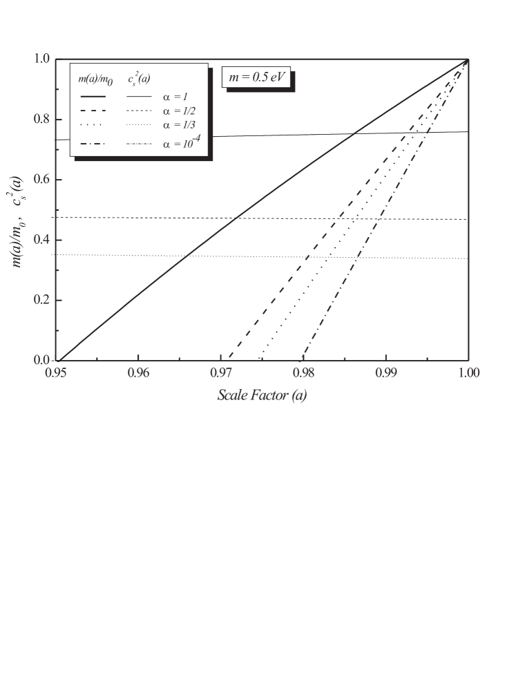
Figure 2: Model independent perturbative modification on squared speed of sound $c^{2}_{s}$ as a function of the scale factor for the neutrino-GCG coupled fluid in comparison with the adiabatic GCG fluid for $A_{s}=0.7$ with $\alpha=1,1/2,\,1/3,\,10^{-4}$, for a present-day value of neutrino mass, $m_{0}=0.5\,eV$.

However, one finds that as far as the perturbative approach is concerned, our model does not run into stability problems in the NR neutrino regime. In opposition, in the SC treatment, where neutrinos are just coupled to dark energy, cosmic expansion in combination with gravitational drag due to cold dark matter have a major impact on the stability of MaVaN models. Usually, for a general fluid for which the equation of state is known, the dominant behaviour on $c_{s}^{2}$ arises from the dark sector component and not by the neutrino component. For the models where the SC (cf. Eq. (33)) implies in a cosmological constant-type equation of state, $p_{\phi}=-\rho_{\phi}$, one inevitably obtains $c_{s}^{2}=-1$.

Thus, the perturbative approach is in agreement with the assumption that the coupling between neutrinos and dark energy (and/or dark matter) is weak. It is found that the stability condition related to the squared speed of sound of the coupled fluid is predominantly governed by dark energy equation of state. This is rather similar to the dynamics of the weakly coupled cosmon fields [47]. Actually, such a troublesome behaviour should have already been observed as the SC implies that $c_{s}^{2}=-1$ from the very start, and the role of recovering the stability is relegated to the neutrino contribution [48]. The loosening of the stationary constraint Eq. (33) emerges from the dynamical dependence on $\varphi$, more concretely due to a kinetic energy component [24]. The knowledge of the background fluid equation of state for the dark sector (the GCG in our example), and the criterion for the applicability of the perturbative approach, do allow to overcome the $c^{2}_{s}$ negative problem, independently from the neutrino mass dependence set by the SC.

4 Coupling to the Higgs field

In order to study the coupling of dark energy to the Higgs field one considers first the coupling of a very light scalar to the Higgs field. One examines a model where the fields are already in their minimum energy configuration (contrary to the usual quintessence models, where the fields are displaced from their minimum). As an example one adopts the minimal spontaneously broken hidden sector model of Schabinger and Wells [29] involving the usual Higgs doublet $H$ and a further singlet complex scalar field $\Phi$ with a potential

$$V(\Phi,H)=-m_{H}^{2}|H|^{2}-m_{\Phi}^{2}|\Phi|^{2}+\lambda|H|^{4}+\rho|\Phi|^{4}+\eta|H|^{2}|\Phi|^{2}.$$ (39)

The fields develop non-vanishing vacuum expectation values, $\langle|H|^{2}\rangle=v^{2}/2$ and $\langle|\Phi|^{2}\rangle=\xi^{2}/2$, and in unitary gauge, the physical fields $h=H-v/\sqrt{2}$ (the Higgs boson field) and $\phi=\Phi-\xi/\sqrt{2}$ mix through a non-diagonal mass matrix due to a non-vanishing $\eta$. The mixing angle $\omega$ between the two scalars is given by

$$\tan\omega={\eta v\xi\over(\rho\xi^{2}-\lambda v^{2})\pm\sqrt{(\rho\xi^{2}-\lambda v^{2})^{2}+\eta^{2}v^{2}\xi^{2}}}~{}.$$ (40)

In order to derive bounds on the mixing $\omega$ one considers fifth force constraints [49]. The mixing of the SM Higgs field with a light scalar induces a long range Yukawa-like interaction due to the exchange of an ultra-light singlet field with strength $g_{e}\sin\omega$ for electrons and $g_{N}\sin\omega$ for nucleons, where $g_{e}=2.9\times 10^{-6}$ is the electron Yukawa coupling and $g_{N}=2.1\times 10^{-3}$ is the nucleon Yukawa coupling [50].

Thus, a non-relativistic test body of mass $M$ placed in the gravitational field of the Earth (with mass $M_{E}$) at a distance $r$ from its center undergoes an acceleration given by:

$$a=a_{gr}+a_{\phi}~{},$$ (41)

where

$$a_{gr}={M_{E}\over M_{Pl}^{2}r^{2}}~{},$$ (42)

is the usual Newtonian acceleration, $M_{Pl}$ is the Planck mass and

$$a_{\phi}={\omega^{2}\over Mr^{2}}[g_{N}^{2}N_{N}^{E}N_{N}^{t}+g_{N}g_{e}(N_{N}^{E}N_{e}^{t}+N_{e}^{E}N_{N}^{t})+g_{e}^{2}N_{e}^{E}N_{e}^{t}]$$ (43)

is the extra acceleration due to a new force arising from $\phi$ exchange, as long as $m_{\Phi}r\ll 1$; $N_{(N,e)}^{(E,t)}$ is the number of nucleons or electrons in the Earth and in the test body.

With these definitions one finds that the difference in acceleration between two test bodies of distinct compositions is given by

$$\varepsilon=2{|a_{1}-a_{2}|\over|a_{1}+a_{2}|}={M_{Pl}\over\bar{m}}\omega^{2}g_{N}g_{e}\Delta f_{p}$$ (44)

where $\bar{m}$ is the average nucleon mass and $\Delta f_{p}$ is the difference in isotopic composition of the two test bodies:

$$\Delta f_{p}={N_{p}^{(1)}\over N_{p}^{(1)}+N_{n}^{(1)}}-{N_{p}^{(2)}\over N_{p}^{(2)}+N_{n}^{(2)}}$$ (45)

with $N_{(p,n)}$ being the number of protons or neutrons in the test body.

For typical isotopic differences of the order of $\Delta f_{p}={\cal O}(10^{-1})$ and using the experimental result $\varepsilon<{\cal O}(10^{-13})$ [51, 52] one gets an estimate for upper bound on the mixing angle

$$\omega<{\cal O}(10^{-20})~{}.$$ (46)

Hence the mixing of an ultra-light scalar singlet is severely constrained by fifth force-type experiments. However, one should point out that this is expected in the discussed model, since in the limit $\xi\ll v$ the mixing angle is given by

$$|\omega|\simeq{\eta\over 2\lambda}{\xi\over v}\simeq\eta{m_{\phi}\over m_{H}}$$ (47)

where one assumes quartic couplings of $\cal{O}$(1). In order for this limit to apply, the Compton length of the light scalar should be of the order of the Earth radius, implying in a mass of the order of $10^{-14}$ eV, to be compared with a Higgs mass of the order of $100$ GeV. This leads to $\omega\simeq\eta\times 10^{-25}$. Therefore, one concludes that there are no limits on the mixing constant $\eta$, which implies that it is possible that the Higgs may have a large invisible width into very light particles.

It is also possible that these light scalars are dark matter candidates. Since in this case there is no symmetry preventing $\phi$ decay, one must check whether in fact they can survive till present. The light scalar decays through its mixing with the Higgs boson. If $m_{\phi}<2m_{e}$, the dominant decay rate is into photons dominated by a top quark triangle ($g_{\phi\bar{t}t}=\omega g_{h\bar{t}t}$), which can be readily estimated:

$$\Gamma(\phi\rightarrow\gamma\gamma)\simeq\omega^{2}\left({\alpha\over\pi}\right)^{2}{G_{F}m_{\phi}^{3}\over 36\sqrt{2}\pi}$$ (48)

which implies that

$$\Gamma(\phi\rightarrow\gamma\gamma)^{-1}\simeq{10^{-3}\over\omega^{2}(m_{\phi}/\mbox{\footnotesize{1 eV}})^{3}}t_{U}$$ (49)

where $t_{U}\simeq 10^{17}s$ is the age of the universe. Hence, in order for the light scalar to survive till present one must require

$$\omega^{2}\left({m_{\phi}\over 1~{}eV}\right)^{3}<10^{-3}$$ (50)

which is easily satisfied for the considered case.

Hence one should consider the bounds discussed in Ref. [36], whose reasoning shows that the scalar $\phi$ cannot be a dark matter candidate. In order to do that one considers the cosmological evolution of the light scalar field. If $\eta$ is sufficiently small, the singlet field decouples early in the thermal history of the universe and is diluted by subsequent entropy production. In Ref. [34], one has considered out-of-equilibrium singlet production via inflaton decay in the context of $N=1$ supergravity inflationary models (see. e.g. [36] and references therein).

On the other hand, for certain values of the coupling $\eta$, it is possible that $\Phi$ particles are in thermal equilibrium with ordinary matter. In order to determine whether this is the case, one makes the usual comparison between the thermalization rate $\Gamma_{th}$ and the expansion rate of the universe, $H$. In Ref. [34] it was found that if $\eta>10^{-10}$ the singlets can be brought into thermal equilibrium right after the electroweak phase transition, being therefore as abundant as photons.

Since one is interested in a stable ultra-light singlet field, it is a major concern avoiding its overproduction if it decouples while relativistic. In fact, in this case, there is an analogue of Lee-Weinberg limit for neutrinos (see e.g. [53]):

$$\Omega_{\phi}h^{2}\simeq 0.08\left({m_{\phi}\over 1~{}\mbox{eV}}\right)\quad,$$ (51)

which shows that as $m_{\phi}\simeq 10^{-14}$ eV, the thermally produced ultra-light scalar $\phi$ particles cannot be a dark matter candidate, as for it is required that $\Omega_{\phi}h^{2}\simeq 0.1$. Of course, this model requires a considerable fine-tuning to generate the different scalar mass scales and it should be embedded in a more encompassing model, such as the Minimal Supersymmetric Standard Model with the addition of one singlet chiral superfield [54].

In what follows one considers the case where the Higgs is coupled to a quintessence field and pay special attention to the fact that it is not settled in its minimum. It is in this respect that a realistic dark energy candidate differs from the generic dark matter candidate modelled by a scalar $\Phi$ considered above .

The most natural potential coupling the Higgs field to the quintessence field is of the “hybrid inflation” type [55]:

$$V(\Phi,H)=U(\Phi)+\lambda\left(|H|^{2}-{v^{2}\over 2}\right)^{2}+\lambda_{1}\Phi^{2}|H|^{2}$$ (52)

where $U(\Phi)$ is the usual quintessential-type potential which can, for instance, be of the form of an exponential or an inverse power law in the singlet field [56, 57]. The second term is the SM Higgs potential and the last term gives rise to Higgs-quintessence coupling, where $\lambda_{1}$ is a dimensionless coupling constant.

Working in the unitary gauge and denoting $\tilde{h}$ as the Higgs field, one can expand the fields around their classical, homogeneous vacuum configurations:

$$\Phi(\vec{x},t)=\phi_{c}(t)+\varphi(\vec{x},t);\;\;\tilde{h}(\vec{x},t)={1\over\sqrt{2}}(\tilde{h}_{c}(t)+h(\vec{x},t))$$ (53)

with $\langle\Phi(\vec{x},t)\rangle=\phi_{c}(t)$, $\langle\tilde{h}(\vec{x},t)\rangle=\tilde{h}_{c}(t)/\sqrt{2}$ and the physical fields have zero vacuum expectation values, $\langle\varphi(\vec{x},t)\rangle=\langle h(\vec{x},t))\rangle=0$.

The classical field configurations obey the equations of motion:

$$\ddot{\phi}_{c}+3H\dot{\phi}_{c}+\left.{dU\over d\Phi}\right|_{\Phi=\phi_{c}}+\lambda_{1}\phi_{c}\tilde{h}_{c}^{2} = 0$$

$$\ddot{\tilde{h}}_{c}+3H\dot{\tilde{h}}_{c}+\lambda(\tilde{h}_{c}^{2}-v^{2})\tilde{h}_{c}+2\lambda_{1}\phi_{c}^{2}\tilde{h}_{c} = 0.$$ (54)

Since this is a model of dynamical dark energy, the classical quintessence field has not relaxed to the minimum of its potential which causes the Higgs field to be displaced from the usual vacuum expectation value ($\tilde{h}_{c}\neq v$, where $v=246$ GeV). This results in a time-varying weak scale or $G_{F}$, for which there are very strong bounds [58, 59] (see also the bound Eq. (18)).

In order to guarantee that $\tilde{h}_{c}=v$, one considers the following ad hoc modifications to the last term of the potential Eq. (52), representing the interaction between the Higgs and quintessence fields:

$$V(\Phi,H)_{int}=\lambda_{1}\Phi^{2}(|H|-v/\sqrt{2})^{2}\;\; (A)$$

$$V(\Phi,H)_{int}=\lambda_{1}(\Phi-\phi_{c})^{2}|H|^{2}\;\; (B)$$

$$V(\Phi,H)_{int}=\lambda_{1}(\Phi-\phi_{c})^{2}(|H|-v/\sqrt{2})^{2}\;\; (C)$$ (55)

For case (A) the equations of motion become:

$$\ddot{\phi}_{c}+3H\dot{\phi}_{c}+\left.{dU\over d\Phi}\right|_{\Phi=\phi_{c}}+\lambda_{1}\phi_{c}(\tilde{h}_{c}-v)^{2} = 0$$

$$\ddot{\tilde{h}}_{c}+3H\dot{\tilde{h}}_{c}+\lambda(\tilde{h}_{c}^{2}-v^{2})\tilde{h}_{c}+\sqrt{2}\lambda_{1}\phi_{c}^{2}(\tilde{h}_{c}-v) = 0$$

and hence $\tilde{h}_{c}=v$ is a solution in which case the classical quintessence field obeys the usual equation:

$$\ddot{\phi}_{c}+3H\dot{\phi}_{c}+\left.{dU\over d\Phi}\right|_{\Phi=\phi_{c}}=0.$$ (57)

It is interesting to notice that this vacuum state for the $\Phi$ field does not arise from a mechanism of spontaneous symmetry breaking, but is instead a consequence of initial conditions for the slow roll evolution of the quintessence field. For most of the models $\phi_{c}$ evolves essentially as a logarithm of the cosmic time, so that its typical rate of change is the Hubble time:

$${\dot{\phi}_{c}\over\phi_{c}}\sim H~{}.$$ (58)

Thus, $\phi_{c}$ evolves in a quasi-stationary regime set by the Hubble scale.

The Lagrangian density for the physical fields is given by

$${\cal L}={1\over 2}\left[(\dot{\phi}_{c}+\dot{\varphi})^{2}-(\vec{\nabla}\varphi)^{2}\right]+{1\over 2}(\partial_{\mu}h)^{2}-V(\phi_{c},v,\varphi,h)$$ (59)

where

$$V(\phi_{c},v,\varphi,h) = U(\phi_{c}+\varphi)+\lambda\left({1\over 2}(h+v)^{2}-v^{2}/2\right)^{2}+$$ (60)

$${\textstyle{{1}\over{2}}}\lambda_{1}(\phi_{c}+\varphi)^{2}h^{2}.$$

Writing

$$U(\phi_{c}+\varphi)=U(\phi_{c})+U^{\prime}(\phi_{c})\varphi+{\textstyle{{1}\over{2}}}U^{\prime\prime}(\phi_{c})\varphi^{2}+{\textstyle{{1}\over{6}}}U^{\prime\prime\prime}(\phi_{c})\varphi^{3}+\cdots$$ (61)

and using the classical equation of motion to cancel the tadpole in Eq. (61) with the $\dot{\phi}_{c}\dot{\varphi}$ term in Eq. (59) one finally obtains:

$${\cal L} = \left[{\textstyle{{1}\over{2}}}\dot{\phi}_{c}^{2}-U(\phi_{c})\right]+{\textstyle{{1}\over{2}}}(\partial_{\mu}\varphi)^{2}+{\textstyle{{1}\over{2}}}(\partial_{\mu}h)^{2}-{\textstyle{{1}\over{2}}}m_{\varphi}^{2}\varphi^{2}-$$

$$\lambda(h^{2}/2+vh)^{2}-{\textstyle{{1}\over{2}}}\lambda_{1}(\phi_{c}+\varphi)^{2}h^{2}-{\textstyle{{1}\over{6}}}g\varphi^{3}+{\cal O}(\varphi^{4})$$

where $m_{\varphi}^{2}=U^{\prime\prime}(\phi_{c})$ and $g=U^{\prime\prime\prime}(\phi_{c})$.

The term in brackets in Eq. (LABEL:L2) reflects the classical zero mode contribution of the scalar field to the energy density of the universe which causes its accelerated expansion. The other terms express the behaviour of the quantum excitations (particles) in the universe. In particular, the Higgs-quintessence interaction results in a new, time-dependent contribution to the Higgs boson mass given by:

$$m_{h}^{2}=2\lambda v^{2}+\lambda_{1}\phi_{c}^{2}~{}.$$ (63)

Since in usual quintessence models $\phi_{c}={\cal O}(M_{Pl})$ one expects a very large deviation from the Standard Model value of the Higgs mass unless the coupling constant $\lambda_{1}$ is very tiny, $\lambda_{1}={\cal O}(v^{2}/M_{Pl}^{2})$ practically closing the Higgs portal. Notice, however, that unitarity in longitudinal gauge boson scattering is not violated since the relevant couplings are still small even if the Higgs boson mass is large.

In case (B) the only difference arises in the interaction term, which becomes

$${\cal L}_{int}=-{\textstyle{{1}\over{2}}}\lambda_{1}\varphi^{2}(v+h)^{2}$$ (64)

and there is no new contribution to the Higgs mass. Interestingly, in this case the coupling generates a new contribution to the mass of the quintessence particle $\varphi$:

$$m_{\varphi}^{2}=U^{\prime\prime}(\phi_{c})+\lambda_{1}v^{2}$$ (65)

that, contrary to usual quintessence models, does not have to be small, since it does not affect the evolution of $\phi_{c}(t)$ given by Eq. (57). Furthermore, since the original quintessence field is not coupled to ordinary matter and there is no mixing to the Higgs boson, there are no bounds arising from fifth force constraints. Notice that in strict terms, this choice renders an ill defined field theory as the $\varphi$ mass will vary on a cosmological scale. However, for models where the acceleration of the expansion is transient, it is possible that $U^{\prime\prime}(\phi_{c})$ vanishes around present time (see e.g. Refs. [60, 61, 62]). Under this condition, this case also introduces a trilinear coupling $\varphi^{2}h$ which, in addition to generating an invisible Higgs boson decay, can bring the quintessence particle into thermal equilibrium in the early universe. The analysis of the contribution arising from this quintessence particle to the dark matter component follows that of Ref. [33, 36, 37]. An interesting situation occurs for the natural case of $\lambda_{1}={\cal O}(0.04)$, which implies $m_{\varphi}\simeq 50$ GeV. In this case, the $\varphi$ particle can be brought into thermal equilibrium through the Higgs coupling in the early universe and, for a Higgs mass $m_{H}\simeq 140$ GeV it decouples while non-relativistic, generating the dark matter density in the observed range.

Therefore, in this unified picture, dark energy is the zero-mode classical field $\phi_{c}(t)$ rolling down the usual quintessence potential and the dark matter candidate is the quantum excitation (particle) $\varphi$, which is produced in the universe due to its coupling to the Higgs boson.

Finally, in case (C) there are no new contributions to either to the Higgs or to the quintessence particle. Only a quartic interaction $\varphi^{2}h^{2}$ is generated and the quintessence particle turns out not to be a good dark matter candidate.

5 Conclusions

In this contribution, the implications of coupling dark energy to SM fields, namely gauge fields, neutrinos and the Higgs field, are examined. One has first considered a possible coupling of dark energy to gauge fields and the impact it might have on the nuclear decay Rutherford-Soddy law. From the available bounds on the variation of the strong and weak gauge couplings it has been estimated, the deviations from the Rutherford-Soddy law. It has been considered a linear model for the variation of the couplings. One finds that the stringent bound on the variation of the weak coupling arising from ${}^{187}Re$ implies in significant constraints on any variation of the Rutherford-Soddy law for weak interactions, actually at the level $3\times 10^{-7}$ for the quintessence field with an exponential potential and at $8\times 10^{-7}$ level for the GCG model. For strong interactions, the bounds are much less stringent and are about $4\times 10^{-2}$ for the quintessence model with exponential potential and of order $10^{-1}$ for the GCG model. Stronger bounds on the deviation of the nuclear decay law for strong interactions could be obtained if variations of the strong coupling were tighter. Furthermore, it is interesting that somewhat different deviations are found for distinct dark energy models. This may be relevant to distinguish them given that most often they are degenerate with respect to the observable cosmological parameters.

In what concerns the coupling of neutrinos to dark energy, one finds that models with increasing neutrino mass with the scale factor is phenomenologically consistent in the context of the GCG model. For $m_{0}=0.5\,eV$, a fairly typical value, one can see that stable MaVaN perturbations correspond to a well defined effective squared speed of sound. The greater the $m_{0}$ values are, the more important are the corrections to the squared speed of sound, up to the limit where the perturbative approach breaks down [24].

As for the coupling of dark energy to the Higgs field, the implications of a scenario where the Higgs boson is coupled to a SM singlet field responsible for the accelerated expansion of the universe were examined. The most natural “hybrid-like” potential is disfavoured since it leads to a time-variation of the weak scale. A modification of the potential can however, give origin to the quite interesting possibility where the classical zero-mode component of the singlet field corresponds to the dark energy particle while its excitation plays the role of dark matter. In order to make this excitation consistent with the cosmological density requirement $\Omega_{\varphi}h^{2}\simeq 0.1$ one gets a coupling to the Higgs field $\lambda_{1}={\cal O}(10^{-2})$, which implies $m_{\varphi}={\cal O}(10)$ GeV. Quite interestingly, this scenario can be be scrutinized in the forthcoming generation of accelerators through the invisible decay of the Higgs boson [25].

O.B would like to thank R. Rosenfeld for collaboration on the work reported on Section 4. He would also like to thank T. Elze for setting up so successfully DICE 2008 and for creating such a nice atmosphere for discussion and fruitful exchange of ideas.

References

References

- [1] Webb J K et al. 1999, Phys. Rev. Lett. 82 884; 2001, 87 091301; Murphy M T, Webb J K, Flambaum V V and Curran S J 2003, Astrophys. Space Sci 283 577.
- [2] Uzan J P 2003, Rev. Mod. Phys. 75 403.
- [3] Bento M C and Bertolami O, arXiv:0901.1818 [astro-ph]
- [4] Bekenstein J D 1982, Phys. Rev. D 25 1527.
- [5] Perlmutter S J et al. (Supernova Cosmology Project) 1999, Ap. J. 517 565; 1998; Riess A G et al., (High-Z Supernova Search Team) 1998, Astron. J. 116 1009; Garnavich P M et al. 1998, Ap. J. 509 74; Tonry J L et al. [Supernova Search Team Collaboration] 2003, Ap. J. 594 1.
- [6] Bento M C, Bertolami O 1999, Gen. Rel. Gravitation 31 1461; Bento M C, Bertolami O, Silva P T 2001, Phys. Lett. B 498 62.
- [7] Bronstein M 1993, Phys. Zeit. Sowejt Union 3 73; Bertolami O 1986, Il Nuovo Cimento 93 B 36; 1986, Forch. Phys. 34 829; Ozer M, Taha M O 1987, Nucl. Phys. B 287 776; Ratra B, Peebles P J E 1988, Phys. Rev. D 37 3406; 1988, Ap. J. Lett. 325 117; Wetterich C 1988, Nucl. Phys. B 302 668; Caldwell R R, Dave R, Steinhardt P J 1998, Phys. Rev. Lett. 80 1582; Zlatev I, Wang L, Steinhardt P J 1999, Phys. Rev. Lett. 82 986; Uzan J P 1999, Phys. Rev. D 59 123510; Bertolami O, Martins P J 2000, Phys. Rev. D 61 064007; Fujii Y 2000, Phys. Rev. D 61 023504; Sen A A, Sen S, Sethi S 2001, Phys. Rev. D 63 107501; Bento M C, Bertolami O, Santos N C 2002, Phys. Rev. D 65 067301.
- [8] Kamenshchik A, Moshella U and Pasquier V 2001, Phys. Lett. B 511 265; Bilić N, Tupper G B and Viollier R D 2002, Phys. Lett. B 535 17; Bento M C, Bertolami O and Sen A A 2002, Phys. Rev. D 66 043507.
- [9] Bento M C, Bertolami O and Sen A A 2003, Phys. Rev. D 67 063003; 2003, Phys. Lett. B 575 172; 2003, Gen. Relativity and Gravitation 35 2063.
- [10] Barreiro T, Bertolami O and Torres P 2008, Phys. Rev. D 78 043530.
- [11] Alcaniz J S, Jain D, and Dev A 2003, Phys. Rev. D 67 043514.
- [12] Bertolami O, Sen A A, Sen S and Silva P T 2004, Mon. Not. Roy. Astron. Soc. 353 329.
- [13] Bento M C, Bertolami O, Sen A A and Santos N C 2005, Phys. Rev. D 71 063501.
- [14] Silva P T and Bertolami O 2003, Ap. J. 599 829; Dev A, Jain D, Upadhyaya D D and Alcaniz J S 2004, Astron. Astrophys. 417 847.
- [15] Bento M C, Bertolami O, Rebouças M J and Silva P T 2006, Phys. Rev. D 73 043504.
- [16] Bertolami O and Silva P T 2006, Mon. Not. Roy. Astron. Soc. 365 1149.
- [17] Bento M C, Bertolami O and Torres P 2007, Phys. Lett. B 648 14.
- [18] Sandvik H, Tegmark M, Zaldarriaga M and Waga I 2004, Phys. Rev. D 69 123524.
- [19] Bento M C, Bertolami O and Sen A A 2004, Phys. Rev. D 70 083519.
- [20] Gu P, Wang X and Zhang X 2003, Phys. Rev. D 68 087301.
- [21] Fardon R, Nelson A E and Weiner N 2004, JCAP 0410 005.
- [22] Lesgourgues J and Pastor S 2006, Phys. Rept. 429 307.
- [23] Bjaelde O E et al. 2008, JCAP 0801 026.
- [24] Bernardini A E and Bertolami O 2008, Phys. Rev. D 77 083506; 2008, Phys. Lett. B 662 97.
- [25] Bertolami O and Rosenfeld R 2008, Int. J. Mod. Phys. A 23 4817.
- [26] Patt B and Wilczek F, arXiv:hep-ph/0605188.
- [27] van der Bij J J 2006, Phys. Lett. B 636 56.
- [28] Binoth T and van der Bij J J 1997, Z. Phys. C 75 17.
- [29] Schabinger R and Wells J D 2005, Phys. Rev. D 72 093007.
- [30] Barger V, Langacker P, McCaskey M, Ramsey-Musolf M J and Shaughnessy G 2008, Phys. Rev. D 77 035005.
- [31] Eboli O J P and Zeppenfeld D 2000, Phys. Lett. B 495 147.
- [32] Silveira V and Zee A 1985, Phys. Lett. B 161 136.
- [33] McDonald J 1994, Phys. Rev. D 50 3637.
- [34] Bento M C, Bertolami O, Rosenfeld R and Teodoro L 2000, Phys. Rev. D 62 041302.
- [35] Holz D E and Zee A 2001, Phys. Lett. B 517 239.
- [36] Bento M C, Bertolami O and Rosenfeld R 2001, Phys. Lett. B 518 276.
- [37] Burgess C P, Pospelov M and ter Veldhuis T 2001, Nucl. Phys. B 619 709.
- [38] Rutherford S E, Chadwick J and Ellis C 1930, Radiations from Radioactive Substances, Cambridge University Press.
- [39] Olive K A and Pospelov M 2008, Phys. Rev. D 77 043524.
- [40] Olive K A and Pospelov M 2002, Phys. Rev. D 65 085044.
- [41] Bento M C, Bertolami O and Santos N M C 2004, Phys. Rev. D 70 107304.
- [42] Olive K A, Pospelov M, Qian Y-Z, Manhes G, Vangioni-Flam E, Coc A and Casse M 2004, Phys. Rev. D 69 027701; Y. Fujii and A. Iwamoto 2003, Phys. Rev. Lett. 91 261101.
- [43] Dent T, Stern S and Wetterich C, arXiv:0809.4628 [hep-ph].
- [44] Ferreira P G and Joyce M 1998, Phys. Rev. D 58 023508.
- [45] Peccei R D 2005, Phys. Rev. D 71 023527.
- [46] Brookfield A W, van de Bruck C, Mota D F and Tocchini-Valentini D 2006, Phys. Rev. D 73 083515.
- [47] Wetterich C 1995, Astron. Astrophys. 301 321.
- [48] Takahashi R and Tanimoto M 2006, JHEP 0605 021.
- [49] Dvali G and Zaldarriaga M 2002, Phys. Rev. Lett. 88 091303.
- [50] Cheng T P 1988, Phys. Rev. D 38 2869.
- [51] Baessler S et al. 1999, Phys. Rev. Lett. 83 3585.
- [52] Adelberger A G 2001, Class. Quant. Gravity 18 2397.
- [53] Kolb E W and Turner M S 1990, The Early Universe Addison-Wesley, Reading MA.
- [54] Balazs C, Carena M, Freitas A and Wagner C E M 2007, JHEP 06 066.
- [55] Linde A D 1994, Phys. Rev. D 49 748.
- [56] Peebles P J E and Ratra B 2003, Rev. Mod. Phys. 75 559.
- [57] Padmanabhan T 2003, Phys. Rept. 380 235.
- [58] Wetterich C 2003, JCAP 0310 002.
- [59] Uzan J P 2003, Rev. Mod. Phys. 75 403.
- [60] Albrecht A and Skordis C 2000, Phys. Rev. Lett. 84 2076.
- [61] Barrow J D, Bean R and Magueijo J 2000, Mon. Not. R. Ast. Soc. 316 L41.
- [62] Bento M C, Bertolami O and Santos N C 2002, Phys. Rev. D 65 067301.