From chiral quark models to high-energy processes

Abstract

We show the results of low-energy chiral quark models for soft matrix elements involving pions and photons. Such soft elements, upon convolution with the hard matrix elements, are relevant in various high-energy processes. We focus on quantities related to the generalized parton distributions of the pion: the parton distribution functions, the parton distribution amplitudes, and the generalized form factors. Wherever possible, the model predictions are confronted with the data or lattice simulations, where surprisingly good agreement is achieved. The QCD evolution from the low quark model scale up to the scale of the data is crucial for this agreement.

12.38.Lg, 11.30, 12.38.-t

Low-energy chiral quark models are designed to describe the the dynamics of the pion and its interactions. Their treatment at the large-$N_{c}$ level is particularly straightforward, as it requires a rather simple task of computing the one-quark-loop diagrams with insertions of pion or gauge-boson vertices. Despite numerous works [1, 2, 3, 4, 5, 6, 7, 8, 9, 10, 11, 12, 13, 14, 15, 16, 17, 18, 19, 20, 21, 22, 23, 24] on the applications of low energy chiral quark models to high-energy processes, their usefulness and predictive power is not well known to the high-energy community. It has been widely believed that because the non-perturbative structure of the pion is such a tremendously difficult problem, it is better to parametrize the matrix elements (for instance, the parton distribution function) by some suitable form. Then this form is inserted as the initial condition to the QCD evolution equations, which bring it to the relevant and experimentally accessible scales. Clearly, that way one can only relate the quantities at different scales and probe the evolution itself, but no genuine non-perturbative dynamics present in the soft matrix elements is investigated. In the case of the pion its low energy properties are expected to be dominated by the spontaneous breakdown of the chiral symmetry, a feature which is implemented in chiral quark models but is largely ignored in many high energy studies.

In our approach two basic elements are crucial: the low-energy dynamical quark model itself, as well as the QCD em evolution, moving the model predictions from the low quark model scale to higher scales, where the experimental or lattice data are available. Without an operational definition of the low energy scale $Q_{0}$ and the QCD evolution relating $Q_{0}$ to $Q$ one cannot compare the model predictions to the data at the scale $Q$. This talk is mainly based on results published recently in Refs. [25, 26].

The theoretical framework is set by the Generalized Parton Distributions (GPDs) [27, 28, 29, 30, 31, 32, 33, 34, 35]. For the case of the pion, the GPD for the non-singlet channel is defined as (we omit the gluon gauge link operators, absent in the light-cone gauge)

$$\epsilon_{3ab}\,{\cal H}^{q,I=1}(x,\zeta,t)\!=\!\!\int\frac{dz^{-}}{4\pi}e^{ixp^{+}z^{-}}\!\!\!\!\left.\langle\pi^{b}(p^{\prime})|\bar{\psi}(0)\gamma^{+}\psi(z)\,\tau_{3}|\pi^{a}(p)\rangle\right|_{z^{+}=0,z^{\perp}=0},$$

while in the singlet case

$$\delta_{ab}\,{\cal H}^{q,I=0}(x,\zeta,t)\!\!=\!\!\!\int\!\!\frac{dz^{-}}{4\pi}e^{ixp^{+}z^{-}}\!\!\!\!\left.\langle\pi^{b}(p^{\prime})|\bar{\psi}(0)\gamma^{+}\psi(z)|\pi^{a}(p)\rangle\right|_{z^{+}=0,z^{\perp}=0}$$

$$\delta_{ab}\,{\cal H}^{g}(x,\zeta,t)\!\!=\!\!\!\int\!\!\frac{dz^{-}}{4\pi p^{+}}e^{ixp^{+}z^{-}}\!\!\!\!\left.\langle\pi^{b}(p^{\prime})|F^{+\mu}(0)F^{+}_{~{}\mu}(z)|\pi^{a}(p)\rangle\right|_{z^{+}=0,z^{\perp}=0},$$

where the kinematics is set by $p^{\prime}=p+q$, $p^{2}=m_{\pi}^{2}$, $q^{2}=-2p\cdot q=t$, and $\zeta=q^{+}/p^{+}$, which denotes the momentum transfer along the light cone. GPDs provide very rich information of the structure of hadrons, which may eventually come from such exclusive processes as $ep\to ep\gamma$, $\gamma p\to pl^{+}l^{-}$, $ep\to epl^{+}l^{-}$, or from the lattice calculations.

Formal properties of GPDs are most elegantly written in the symmetric notation: $\xi=\frac{\zeta}{2-\zeta}$, $X=\frac{x-\zeta/2}{1-\zeta/2}$, with $0\leq\xi\leq 1$, $-1\leq X\leq 1$, where one finds

$$H^{I=0}(X,\xi,t)=-H^{I=0}(-X,\xi,t),\;H^{I=1}(X,\xi,t)=H^{I=1}(-X,\xi,t).$$ (3)

For $X\geq 0$ one has

$${\cal H}^{I=0,1}(X,0,0)=q^{S,NS}(X),$$ (4)

with $q(x)^{i}$ being the standard parton distribution functions (PDFs). The following sum rules hold:

$$\forall\xi: \int_{-1}^{1}\!\!\!\!\!dX\,{H}^{I=1}(X,\xi,t)=2F_{V}(t),$$

$$\int_{-1}^{1}\!\!\!\!\!dX\,X\,{H}^{I=0}(X,\xi,t)=2\theta_{2}(t)-2\xi^{2}\theta_{1}(t),$$

where $F_{V}(t)$ is the electromagnetic form factor, while $\theta_{1}(t)$ and $\theta_{2}(t)$ are the gravitational form factors [36], related, correspondingly, to the charge conservation and to the momentum sum rule in the deep inelastic scattering.

More generally, the polynomiality conditions [27], following from the Lorentz invariance, time reversal, and hermiticity, state that

$$\int_{-1}^{1}\!\!\!\!\!dX\,X^{2j}\,{H}^{I=1}(X,\xi,t)=2\sum_{i=0}^{j}A_{2j+1,2i}(t)\xi^{2i},$$

$$\int_{-1}^{1}\!\!\!\!\!dX\,X^{2j+1}\,{H}^{I=0}(X,\xi,t)=2\sum_{i=0}^{j+1}A_{2j+2,2i}(t)\xi^{2i},$$

where $A$’s are the generalized form factors (GFFs). These form factors can be also expressed as matrix elements of the form

$$\left<\pi^{+}(p^{\prime})\right|\overline{u}(0)\,\gamma^{\{\mu}\,i\raisebox{0.89996pt}{$\stackrel{{\scriptstyle\scriptstyle\leftharpoonup\rightharpoonup}}{{D}}$}\/^{\mu_{1}}i\raisebox{0.89996pt}{$\stackrel{{\scriptstyle\scriptstyle\leftharpoonup\rightharpoonup}}{{D}}$}\/^{\mu_{2}}\dots i\raisebox{0.89996pt}{$\stackrel{{\scriptstyle\scriptstyle\leftharpoonup\rightharpoonup}}{{D}}$}\/^{\mu_{n-1}\}}\,u(0)\left|\pi^{+}(p)\right>=$$

$$\;\;\;\;2P^{\{\mu}P^{\mu_{1}}\dots P^{\mu_{n-1}\}}A_{n0}(t)+$$

$$2\sum^{n}_{k=2,4,\dots}q^{\{\mu}q^{\mu_{1}}\dots q^{\mu_{k-1}}P^{\mu_{k}}\dots P^{\mu_{n-1}\}}\,2^{-k}A_{nk}(t),$$ (5)

where $P=p^{\prime}+p$, hence the GPDs may be viewed as an infinite collection of GFFs. The positivity bound [37, 38] states that

$$|H_{q}(X,\xi,t)|\leq\sqrt{q(x_{\rm in})q(x_{\rm out})},\;\;\;\;\;\xi\leq X\leq 1,$$ (6)

where $x_{\rm in}=(x+\xi)/(1+\xi)$, $x_{\rm out}=(x-\xi)/(1-\xi)$. Finally, a low-energy theorem [39]

$$H_{I=1}(2z-1,1,0)=\phi(z)$$ (7)

holds, relating the GPD to the pion distribution amplitude (DA), denoted as $\phi$.

We stress that the above-listed relations and bounds impose severe constraints on the possible form of the GPDs. All these formal requirements are naturally satisfied in our quark-model calculations [25].

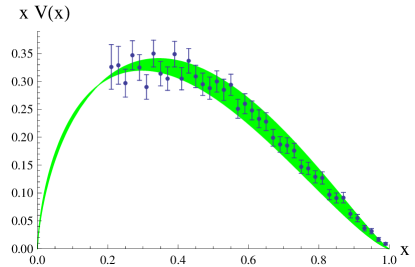
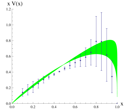
Figure 1: Left: model prediction for the valence parton distribution in the pion evolved to the scale of $Q=4$ GeV (band). The width of the band indicates the uncertainty in the initial scale $Q_{0}$, Eq. (9). The data points come from the Drell-Yan E615 experiment [40]. Right: same, evolved to the scale $Q=0.35~{}{\rm GeV}$. The data come from the transverse lattice calculations of Ref. [41]

With $\zeta=t=0$, the GPD becomes the usual PDF, cf. Eq. (4). Long ago Davidson and one of us (ERA) found that in the Nambu–Jona-Lasinio model [1] ${q(x)=1}$. This result pertains to the low-energy chiral-quark-model scale, which is a priori not known and has to be determined. At this scale the gluons have been integrated out and effective quark degrees of freedom are the only degrees of freedom. Thus, all observables are saturated by the quark contribution, in particular, the momentum sum rule. From experiment, the momentum fraction carried by the valence quarks is [42, 43]

$$\langle x\rangle_{v}=0.47(2){\rm~{}~{}at~{}~{}}Q^{2}=4~{}{\rm GeV}^{2}.$$ (8)

We evolve this value backward with the LO DGLAP equations down to the scale where quarks carry all the momentum, $\langle x\rangle_{v}=1$. This procedure, assuming the matching of the quark model results and QCD at the quark model scale, yields the quark model scale

$${Q_{0}=313_{-10}^{+20}{\rm~{}MeV}},$$ (9)

where the range reflects the uncertainty in (8).

We admit that such a low scale, where ${\alpha(Q^{2}_{0})}/({2\pi})=0.34$, makes the evolution very fast for the scales close to the initial value $Q_{0}$. This calls for improvement of the evolution. However, the NLO effects are small [9]. On the other hand, the removal of the Landau pole by means of the analytic QCD method [44, 45, 46, 47] results in a too slow evolution, incapable of reconciling the quark-model results with experimental data. Thus in our studies we employ the simplest LO DGLAP QCD evolution, baring in mind that it is good at intermediate values of $x$.

The results of our procedure for the non-singlet PDF (valence quark distribution) of the pion are shown on the left side of Fig. 1. We have evolved the quark model result (8) from the scale (9) up to the scale $Q=4$ GeV corresponding to the E615 experiment [40]. We note a very reasonable agreement for all the range where the data are available. On the right side we show the same quantity evolved to the rather low scale of $Q=350$ MeV and confronted with the transverse lattice data [41]. Again, the agreement is quite remarkable, showing the features of transverse-lattice calculation, designed to work at low-energy scales.

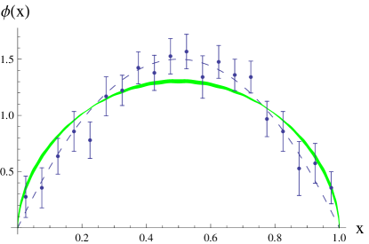
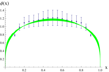
Figure 2: Left: model prediction for the pion distribution amplitude evolved to the scale $Q=2~{}{\rm GeV}$ (band) and compared to the E791 di-jet measurement [48]. The width of the band indicates the uncertainty in the initial scale $Q_{0}$, Eq. (9). The dashed line shows the asymptotic form $\phi(x,\infty)=6x(1-x)$. Right: same evolved to the scale $Q=0.5{\rm GeV}$ compared to the transverse lattice data [41].

Next, we look at the DA, related to the GPD via the sum rule (7). Here the evolution is carried out with the LO ERBL equations. The results are displayed in Fig. 2, again in fair agreement with the data, especially for the lattice case on the right-hand side. Thus the GPDs for the special kinematic cases of Eqs. (4,7) are well reproduced in chiral quark models supplied with evolution.

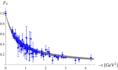
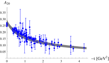
Figure 3: The electromagnetic form factor (left) and the quark part of the gravitational form factor, $A_{20}$ (right) in the Spectral Quark Model compared to the lattice data from Ref. [49]. The band around the model curve indicates the uncertainty in the quark momentum fraction and the $m_{\rho}$ parameter in the Spectral Quark Model.

In Ref. [25] we provide expressions for the full form of the GPDs in the NJL model and in the Spectral Quark Model [50]. These expressions have a non-trivial structure, in particular they do not exhibit factorization in the $t$ and $x$ variables, while satisfying all formal requirements listed above, including polynomiality. Since there is no data for the full kinematic range for the GPDs, we display the results for the generalized form factors. Interestingly, there is recent information on these objects from the full QCD on the lattice [49, 51]. The Spectral Quark Model vector form factor and the quark part of the gravitational form factor of the pion, $A_{20}$, are compared to these lattice data in Fig. 3. We note a very good agreement. In the Spectral Quark Model the expressions are particularly simple,

$$F_{V}^{\rm SQM}(t) = \frac{m_{\rho}^{2}}{m_{\rho}^{2}-t},$$ (10)

$$\ \theta_{1}^{\rm SQM}(t) = \theta^{\rm SQM}_{2}(t)=\frac{m_{\rho}^{2}}{t}\log\left(\frac{m_{\rho}^{2}}{m_{\rho}^{2}-t}\right).$$

We note the longer tail of the gravitational form factor in the momentum space, meaning a more compact distribution in the coordinate space. Explicitly, in the considered chiral quark models we find the simple relation

$$2\langle r^{2}\rangle_{\theta}=\langle r^{2}\rangle_{V}.$$ (11)

In Fig. 4 we show our predictions for the higher-order generalized form factors, evolved to the scale of 2 GeV. In Ref. [52] we have pointed out that these moments evolve in a very simple way with the LO DGLAP-ERBL evolution. One finds triangular structures, for instance in the non-singlet odd-$n$ case

$$A_{10}(t,Q)=L_{1}A_{10}(t,Q_{0}),$$

$$A_{32}(t,Q)=\frac{1}{5}(L_{1}-L_{3})A_{10}(t,Q_{0})+L_{3}A_{32}(t,Q_{0}),$$

$$A_{54}(t,Q)=\frac{1}{105}(9L_{1}-14L_{3}+5L_{5})A_{10}(t,Q_{0})$$

$$\;\;\;\;+\frac{2}{3}(L_{3}-L_{5})A_{32}(t,Q_{0})+L_{5}A_{54}(t,Q_{0}),$$

$$\dots$$

$$A_{30}(t,Q)=L_{3}A_{30}(t,Q_{0}),$$

$$A_{52}(t,Q)=\frac{2}{3}(L_{3}-L_{5})A_{30}(t,Q_{0})+L_{5}A_{52}(t,Q_{0}),$$

$$\dots$$

$$A_{50}(t,Q)=L_{5}A_{50}(t,Q_{0}),$$

$$\dots$$ (12)

where

$$L_{n}=\left(\frac{\alpha(Q^{2})}{\alpha(Q_{0}^{2})}\right)^{\gamma_{n-1}/(2\beta_{0})},$$ (13)

and $\gamma_{i}$ denotes anomalous dimensions, in the present case for the vector operator. Certainly, $L_{1}=1$, and the vector form factor, corresponding to a conserved current, does not evolve. Similarly, the gravitational form factors do not evolve. The higher-order form factors, however, do change due to evolution. Similar structures of equations to (12) appear for the even $n$, as well as for the singlet case [52]. At the moment, there is no data to compare to for the higher-order form factors, but our predictions of Fig. 4 can be tested in future lattice studies.

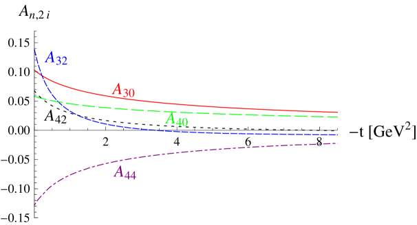
Figure 4: (Predictions for the higher-order generalized form factors $A_{3,2i}$ and $A_{4,2i}$ of the pion from the Spectral Quark Model evolved to the scale $Q=2$ GeV.

However, already at present there exists useful information at $t=0$. Below we compare our model values of the higher-order form factors at $t=0$ to the lattice data provided in Sec. 7 of Ref. [49]. With the short-hand notation $\langle x^{n}\rangle=A_{n+1,0}(0)$ one finds that at the lattice scale of $Q=2$ GeV

$$\langle x\rangle=0.271\pm 0.016,$$ (14)

$$\langle x^{2}\rangle=0.128\pm 0.018,$$

$$\langle x^{3}\rangle=0.074\pm 0.027.\;\;\;(\rm lattice)$$

while in the chiral quark models we get, after the LO DGLAP evolution to the lattice scale,

$$\langle x\rangle=0.28\pm 0.02,$$ (15)

$$\langle x^{2}\rangle=0.10\pm 0.02,$$

$$\langle x^{3}\rangle=0.06\pm 0.01.\;\;\;(\rm chiral~{}quark~{}models)$$

The model error bars come from the uncertainty of the scale $Q_{0}$ in Eq. (9). As we can see, the agreement falls within the error bars.

To briefly summarize the results presented in this talk, we state that the chiral quark models supplied with the QCD evolution work well for a wide variety of quantities related to the GPDs of the pion. Thus they may provide valuable insight into the non-perturbative dynamics behind the soft matrix elements. Further details can be found in Refs. [25, 26].

Since at this meeting we are remembering Professor Jan Kwieciński, I wish to end my contribution by showing one of the last photos of our dear teacher and friend sitting happily among his colleagues. The picture was taken on the occasion of handling to Jan the issue of Acta Physica Polonica B [53] (placed at the corner of the table) dedicated to him in honor of his 65th birthday. The event took part in the Institute of Nuclear Physics in June 2003, just two and a half months before his premature passing away. We all miss you, Jan!

Supported in part by the Polish Ministry of Science and Higher Education, grants N202 034 32/0918 and N202 249235, Spanish DGI and FEDER funds with grant FIS2008-01143/FIS, Junta de Andalucía grant FQM225-05, and the EU Integrated Infrastructure Initiative Hadron Physics Project, contract RII3-CT-2004-506078.

Figure 5: 12 June 2003, left to right: Mariusz Sadzikowski, Wojciech Florkowski, Michał Praszałowicz, Kacper Zalewski, Krzysztof Golec-Biernat, Andrzej Białas, Jan Kwieciński, Maria and Wiesław Czyż.

References

- [1] R.M. Davidson and E. Ruiz Arriola, Phys. Lett. B348 (1995) 163.
- [2] A.E. Dorokhov and L. Tomio, (1998), hep-ph/9803329.
- [3] M.V. Polyakov and C. Weiss, Phys. Rev. D59 (1999) 091502, hep-ph/9806390.
- [4] M.V. Polyakov and C. Weiss, Phys. Rev. D60 (1999) 114017, hep-ph/9902451.
- [5] A.E. Dorokhov and L. Tomio, Phys. Rev. D62 (2000) 014016.
- [6] I.V. Anikin et al., Nucl. Phys. A678 (2000) 175.
- [7] I.V. Anikin et al., Phys. Atom. Nucl. 63 (2000) 489.
- [8] E. Ruiz Arriola, (2001), hep-ph/0107087.
- [9] R.M. Davidson and E. Ruiz Arriola, Acta Phys. Polon. B33 (2002) 1791, hep-ph/0110291.
- [10] E. Ruiz Arriola and W. Broniowski, Phys. Rev. D66 (2002) 094016, hep-ph/0207266.
- [11] E. Ruiz Arriola, Acta Phys. Polon. B33 (2002) 4443, hep-ph/0210007.
- [12] M. Praszalowicz and A. Rostworowski, (2002), hep-ph/0205177.
- [13] B.C. Tiburzi and G.A. Miller, Phys. Rev. D67 (2003) 013010, hep-ph/0209178.
- [14] B.C. Tiburzi and G.A. Miller, Phys. Rev. D67 (2003) 113004, hep-ph/0212238.
- [15] L. Theussl, S. Noguera and V. Vento, Eur. Phys. J. A20 (2004) 483, nucl-th/0211036.
- [16] W. Broniowski and E. Ruiz Arriola, Phys. Lett. B574 (2003) 57, hep-ph/0307198.
- [17] M. Praszalowicz and A. Rostworowski, Acta Phys. Polon. B34 (2003) 2699, hep-ph/0302269.
- [18] A. Bzdak and M. Praszalowicz, Acta Phys. Polon. B34 (2003) 3401, hep-ph/0305217.
- [19] S. Noguera and V. Vento, Eur. Phys. J. A28 (2006) 227, hep-ph/0505102.
- [20] B.C. Tiburzi, Phys. Rev. D72 (2005) 094001, hep-ph/0508112.
- [21] W. Broniowski and E.R. Arriola, Phys. Lett. B649 (2007) 49, hep-ph/0701243.
- [22] A. Courtoy and S. Noguera, Phys. Rev. D76 (2007) 094026, 0707.3366 [hep-ph].
- [23] A. Courtoy and S. Noguera, Prog. Part. Nucl. Phys. 61 (2008) 170, 0803.3524 [hep-ph].
- [24] P. Kotko and M. Praszalowicz, (2008), 0803.2847 [hep-ph].
- [25] W. Broniowski, E.R. Arriola and K. Golec-Biernat, Phys. Rev. D77 (2008) 034023, 0712.1012 [hep-ph].
- [26] W. Broniowski and E.R. Arriola, Phys. Rev. D78 (2008) 094011, 0809.1744 [hep-ph].
- [27] X.D. Ji, J. Phys. G24 (1998) 1181, hep-ph/9807358.
- [28] A.V. Radyushkin, (2000), hep-ph/0101225.
- [29] K. Goeke, M.V. Polyakov and M. Vanderhaeghen, Prog. Part. Nucl. Phys. 47 (2001) 401, hep-ph/0106012.
- [30] A.P. Bakulev et al., Phys. Rev. D62 (2000) 054018, hep-ph/0004111.
- [31] M. Diehl, Phys. Rept. 388 (2003) 41, hep-ph/0307382.
- [32] X.D. Ji, Ann. Rev. Nucl. Part. Sci. 54 (2004) 413.
- [33] A.V. Belitsky and A.V. Radyushkin, Phys. Rept. 418 (2005) 1, hep-ph/0504030.
- [34] T. Feldmann, Eur. Phys. J. Special Topics 140 (2007) 135.
- [35] S. Boffi and B. Pasquini, Riv. Nuovo Cim. 30 (2007) 387, 0711.2625 [hep-ph].
- [36] J.F. Donoghue and H. Leutwyler, Z. Phys. C52 (1991) 343.
- [37] B. Pire, J. Soffer and O. Teryaev, Eur. Phys. J. C8 (1999) 103, hep-ph/9804284.
- [38] P.V. Pobylitsa, Phys. Rev. D65 (2002) 077504, hep-ph/0112322.
- [39] M.V. Polyakov, Nucl. Phys. B555 (1999) 231, hep-ph/9809483.
- [40] J.S. Conway et al., Phys. Rev. D39 (1989) 92.
- [41] S. Dalley and B. van de Sande, Phys. Rev. D67 (2003) 114507, hep-ph/0212086.
- [42] P.J. Sutton et al., Phys. Rev. D45 (1992) 2349.
- [43] M. Gluck, E. Reya and I. Schienbein, Eur. Phys. J. C10 (1999) 313, hep-ph/9903288.
- [44] D.V. Shirkov and I.L. Solovtsov, Phys. Rev. Lett. 79 (1997) 1209, hep-ph/9704333.
- [45] N.G. Stefanis, W. Schroers and H.C. Kim, Eur. Phys. J. C18 (2000) 137, hep-ph/0005218.
- [46] A.P. Bakulev et al., Phys. Rev. D70 (2004) 033014, hep-ph/0405062.
- [47] A.P. Bakulev, A.I. Karanikas and N.G. Stefanis, Phys. Rev. D72 (2005) 074015, hep-ph/0504275.
- [48] E791, E.M. Aitala et al., Phys. Rev. Lett. 86 (2001) 4768, hep-ex/0010043.
- [49] D. Brommel, Pion structure from the lattice, PhD thesis, University of Regensburg, Regensburg, Germany, 2007, DESY-THESIS-2007-023.
- [50] E. Ruiz Arriola and W. Broniowski, Phys. Rev. D67 (2003) 074021, hep-ph/0301202.
- [51] D. Brommel et al., PoS LAT2005 (2006) 360, hep-lat/0509133.
- [52] W. Broniowski and E.R. Arriola, Phys. Rev. D79 (2009) 057501, 0901.3336 [hep-ph].
- [53] Acta Phys. Pol. B34(2003) No. 6