Macroeconomic Phase Transitions Detected from the Dow Jones Industrial Average Time Series

Abstract

In this paper, we perform statistical segmentation and clustering analysis of the Dow Jones Industrial Average time series between January 1997 and August 2008. Modeling the index movements and log-index movements as stationary Gaussian processes, we find a total of 116 and 119 statistically stationary segments respectively. These can then be grouped into between five to seven clusters, each representing a different macroeconomic phase. The macroeconomic phases are distinguished primarily by their volatilities. We find the US economy, as measured by the DJI, spends most of its time in a low-volatility phase and a high-volatility phase. The former can be roughly associated with economic expansion, while the latter contains the economic contraction phase in the standard economic cycle. Both phases are interrupted by a moderate-volatility market, but extremely-high-volatility market crashes are found mostly within the high-volatility phase. From the temporal distribution of various phases, we see a high-volatility phase from mid-1998 to mid-2003, and another starting mid-2007 (the current global financial crisis). Transitions from the low-volatility phase to the high-volatility phase are preceded by a series of precursor shocks, whereas the transition from the high-volatility phase to the low-volatility phase is preceded by a series of inverted shocks. The time scale for both types of transitions is about a year. We also identify the July 1997 Asian Financial Crisis to be the trigger for the mid-1998 transition, and an unnamed May 2006 market event related to corrections in the Chinese markets to be the trigger for the mid-2007 transition.

1 Introduction

Most people remember the most recent economic recession as short (lasting only eight months from March 2001 to November 2001 [1]) and mild (affecting mostly high-tech companies). Against this backdrop, there have been many sensationalist claims that the current global financial crisis is the deepest (broad spectrum of economic sectors affected) and longest (peak in December 2007 [1], and a potential trough in March 2009). According to other sources (see, for example, Ref. [2]), however, the Subprime Crisis surfaced around July 2007 with a slew of bad news from subprime lenders, and the Dow Jones Industrial Average (DJI) dipping roughly 1,000 points going from July 2007 to August 2007. Since then, billions of dollars have been sunk into relief and stimulus packages, and governments around the world are planning further aid totalling in excess of a trillion US dollars. There are hardly any positive results to show for the effort thus far, and the reasons can best be summed up as “too little, too late”. In medicine, early intervention is generally more effective and less costly compared to a late cure. The same is probably true for economies and financial markets. Clearly, even if we are not sure what kind of intervention measures will be effective, acting early is still more desirable to acting later. To accomplish this, it is important to be able to unambiguously detect the onset of a financial crisis, so that we can at the same time avoid over-reacting when the market has merely caught a ‘cold’.

Since econometric data such as the gross national product (GNP) are released quarterly, and are adjusted monthly, they are not useful for timely detection. We thus look to higher-frequency financial time series for this sleuth work. Given that each and every financial crisis may have their own unique and esoteric characters, we need a financial time series that is sufficiently representative of the broad spectrum of industries to be able to detect the starting point of these crises. Indices such as the Dow Jones Industrial Average (DJI), Dow Jones Composite Average (DJA), and the Standards & Poors 500 (INX) are most suitable for this purpose. Clearly, detecting the onset of a financial crisis is a change point problem [3, 4]. In their seminal works, Goldfeld et al, Hamilton and Kim et al fitted a Markov-switching model to local trends in the US GNP time series to detect transitions between a macroeconomic phase (or regime) with high growth rate and a macroeconomic phase with low growth rate [5, 6, 7]. Unlike econometric time series, which evolve fairly slowly with time, it is well known that financial time series exhibit dynamics on multiple time scales. To avoid potential complications arising from such multiscale dynamics, we analyze statistical fluctuations in the index time series, instead of looking merely at the local trend, as is done for deciding the duration of an economic recession. For the different macroeconomic phases the economy and financial market can be found in, these statistical flucutations should also be qualitatively different.

In this paper, we describe in Section 2 a model-based approach to statistically segmenting the DJI time series, which is assumed to consist of a large number of statistically stationary segments. Within different segments, the index movements (or log index movements) are assumed to follow stationary Gaussian processes with different means and variances. We then discover these segments using a recursive segmentation scheme based on the relative entropy between them. Following this, we determine the small number of macroeconomic phases represented in the time series by performing agglomerative hierarchical clustering on the segments. In Section 3, we report findings from our statistical segmentation and clustering analyses. Segments obtained using the two models are in good agreement with each other, and also with the dates of major market events, suggesting that the segment boundaries discovered are robust and meaningful. Depending on the model, and the level of granularity we choose, we find between six to seven macroeconomic phases after clustering the segments. These six to seven macroeconomic phases are distinguished primarily by their variances, which represent market volatilities. While the clusters appear to be less robust compared to the segments, their temporal distributions do tell a fairly consistent story: the US market, as measured by the DJI, is found predominantly in a low-volatility phase and a high-volatility phase, corresponding roughly to economic expansion and economic contraction respectively. Both phases are interrupted by a moderate-volatility market correction phase, while the high-volatility phase is also interrupted by an extremely-high-volatility market crash phase. More interestingly, our results suggest that the mid-1998 transition into the high-volatility phase (which lasted five years) was triggered by the 1997 Asian Financial Crisis, whereas the mid-2007 transition into the high-volatility phase (the global financial crisis we find ourselves in right now) was triggered by a 2006 correction in the Chinese markets. As we have guessed, the world is very tightly coupled economically, perhaps even more so than we would like to admit. We then conclude in Section 4, and describe further work we are currently undertaking.

2 Data, Models and Methods

2.1 Data and Models

While it is not as comprehensive as the S&P 500, the Dow Jones Industrial Average (a price-weighted index consisting of 30 of the largest and most widely held public companies in US) is nonetheless a very important index measuring the performance of the US market. Tic-by-tic data for this index between 1 January 1997 and 31 August 2008 was downloaded from the Taqtic database [8], and processed to give a half-hourly time series $\mathbf{X}=(X_{1},X_{2},\dots,X_{N})$, where $X_{t}$ is the index value at the $t$th half-hour, and $N$ is the total number of trading half-hours between 1 January 1997 to 31 August 2008. The half-hourly frequency was chosen so that there is sufficient statistics to identify segments as short as a single day. From the index time series $\mathbf{X}$, we obtain the index movement time series $\mathbf{x}=(x_{1},\dots,x_{N-1})$, where $x_{t}=X_{t}-X_{t-1}$, as well as the log-index movement time series $\mathbf{y}=(y_{1},\dots,y_{N-1})$, where $y_{t}=\log X_{t}-\log X_{t-1}$. We assume that $\mathbf{x}$ and $\mathbf{y}$ consist of $M$ and $M^{\prime}$ statistically stationary segments respectively, where the numbers of segments $M$ and $M^{\prime}$, and where the segments are, are unknown and must be determined through a segmentation procedure.

To do this segmentation, we assume the movements $x_{t}$ within statistically stationary segment $m$ are drawn from a Gaussian (normal) distribution with mean $\mu_{m}$ and variance $\sigma_{m}^{2}$. Similarly, the movements $y_{t}$ within statistically stationary segment $m^{\prime}$ are assumed to be drawn from a Gaussian distribution with mean $\mu^{\prime}_{m^{\prime}}$ and variance ${\sigma^{\prime}_{m^{\prime}}}^{2}$. The log-normal index movement model is popular in the finance literature, where traders are assumed to be influenced mainly by percentage changes rather than absolute changes, because of their constant mental reference to a risk-free interest rate. In this study, we also consider the normal index movement model, in case traders in the real world also pay attention to actual changes in the index. In both models, the movements from one half-hour to the next are uncorrelated, in contrast to real-world financial time series, which are known to exhibit correlations on multiple time scales. For the purpose of finding statistically robust change points in the time series, we believe that the details of the models used will not be important, and the difference between an uncorrelated model versus a correlated model will merely be a difference between statistical significance and signal-to-noise ratio.

2.2 Methods

Time series segmentation schemes can be very broadly classified into those based on pattern recognition, and those based on information-theoretic measures. In pattern-based segmentation schemes, features within the time series are abstracted into symbols, as is frequently done in the technical analysis of stock markets [9]. Segmentation decisions are then based on the relative abundance of symbols, or their context trees [10, 11, 12, 13]. Information-theoretic segmentation methods are popular in image segmentation [14], biological sequence segmentation [15], and also in medical time series analysis [16], but not widely used for financial time series segmentation [17, 18].

To determine the location of the $M$ segments, we employ the recursive segmentation scheme introduced by Bernaola-Galván et al [19, 20] for biological sequence segmentation. In this scheme, we first identify a cursor position $t$ in the sequence $\mathbf{z}=(z_{1},z_{2},\dots,z_{N})$ with length $N$, and compute the Jensen-Shannon divergence

$$\Delta_{t}=\log\frac{P_{2}(t)}{P_{1}},$$ (1)

which measures the statistical divergence between the left subsequence $\mathbf{z}_{L}=(z_{1},z_{2},\dots,z_{t})$ and the right subsequence $\mathbf{z}_{R}=(z_{t+1},z_{t+2},\dots,z_{N})$. Here,

$$P_{1}=\prod_{i=1}^{N}\frac{1}{\sqrt{2\pi\sigma^{2}}}\exp\left[-\frac{(z_{i}-\mu)^{2}}{2\sigma^{2}}\right]$$ (2)

is the likelihood for observing the sequence $\mathbf{z}=(z_{1},z_{2},\dots,z_{N})$, assuming that the entire sequence is generated by a single Gaussian process with mean $\mu$ and variance $\sigma^{2}$, and

$$P_{2}(t)=\prod_{i=1}^{t}\frac{1}{\sqrt{2\pi\sigma_{L}^{2}}}\exp\left[-\frac{(z_{i}-\mu_{L})^{2}}{2\sigma_{L}^{2}}\right]\prod_{j=t+1}^{N}\frac{1}{\sqrt{2\pi\sigma_{R}^{2}}}\exp\left[-\frac{(z_{j}-\mu_{R})^{2}}{2\sigma_{R}^{2}}\right]$$ (3)

is the likelihood for observing the sequence $\mathbf{z}$, assuming that the left subsequence $\mathbf{z}_{L}=(z_{1},z_{2},\dots,z_{t})$ is generated by a Gaussian process with mean $\mu_{L}$ and variance $\sigma_{L}^{2}$, and the right subsequence $\mathbf{z}_{R}=(z_{t+1},z_{t+2},\dots,z_{N})$ is generated by a Gaussian process with mean $\mu_{R}$ and variance $\sigma_{R}^{2}$.

Since the parameters $\mu$, $\mu_{L}$, $\mu_{R}$, $\sigma^{2}$, $\sigma_{L}^{2}$, and $\sigma_{R}^{2}$ are not given, we can replace them with their maximum-likelihood estimates $\hat{\mu}$, $\hat{\mu}_{L}$, $\hat{\mu}_{R}$, $\hat{\sigma}^{2}$, $\hat{\sigma}_{L}^{2}$, and $\hat{\sigma}_{R}^{2}$. These estimates maximizes $P_{1}$ and $P_{2}(t)$ relative to the data, and the Jensen-Shannon divergence, which simplifies to

$$\Delta_{t}=N\log\hat{\sigma}-n_{L}\log\hat{\sigma}_{L}-n_{R}\log\hat{\sigma}_{R}+\frac{1}{2}\geq 0,$$ (4)

tells us how much better the best two-segment model fits the observed data over the best one-segment model. If we now vary $t$, and identify $t=t^{*}$ for which $\Delta_{t^{*}}=\Delta^{*}=\max_{t}\Delta_{t}$, this would tell us the best place to segment the given sequence $\mathbf{z}=(z_{1},z_{2},\dots,z_{N})$. The Jensen-Shannon divergence maximum $\Delta^{*}$ gives us an indication of how significant the segment boundary at $t^{*}$ is statistically.

We then repeat this one-into-two segmentation procedure to recursively cut the given sequence up into shorter and shorter segments. As this recursive segmentation progresses, the divergence maxima for the new cuts will generally become smaller and smaller. At some point, new cuts will no longer be statistically significant, and the segmentation process must be terminated. There are several ways to do this: through hypothesis testing [19, 20], through model selection, [21, 22], or through examination of the intrinsic statistical fluctuations within the sequence to be segmented [23]. In this work, we adopted a semi-automated approach to terminate the recursive segmentation. First, we recursively segment the time series until the divergence maxima of the new cuts fall below a given threshold, selected by inspection to be $\Delta_{0}=10$. We then screen these segments manually, by visually inspecting the Jensen-Shannon divergence spectrum $\Delta_{t}$, to decide whether very short segments should be eliminated, and very long segments should be further segmented.

At each stage of the recursive segmentation, we also perform segmentation optimization, to overcome the context sensitivity problem identified in Ref. [24]. For this, we use the algorithm described in Ref. [23], where we start with $M$ segment boundaries $\{t_{1},\dots,t_{M}\}$ obtained after new cuts have been introduced by the recursive segmentation. To optimize the position of the $m$th segment boundary, we compute the Jensen-Shannon divergence spectrum $\Delta_{t}$ within the supersegment $(x_{t_{m-1}+1},\dots,x_{t_{m+1}})$ bounded by the segments boundaries $t_{m-1}$ and $t_{m+1}$, and replace $t_{m}$ by $t_{m}^{*}$, where the supersegment Jensen-Shannon divergence is maximized. This is done for all $M$ segment boundaries, and iterated until all segment boundaries converge to their optimal positions. We then continue the recursive segmentation with this optimized set of segments, introducing new cuts, optimize the new segment boundaries along with the old segment boundaries, until the segmentation is terminated.

Finally, after we are satisfied that the final segmentation is optimal, and the segment boundaries are all statistically significant, we perform agglomerative hierarchical clustering on the segments to determine the number of macroeconomic phases represented in the time series. This is done with the complete link algorithm [25], using the Jensen-Shannon divergences between segments as their statistical distances. Clustering of different periods within a financial time series has been previously investigated [26, 27, 28], but we believe we are the first to incorporate a rigorous segmentation analysis into such a study.

3 Results and Discussions

3.1 Statistical Segmentation

From the DJI time series between January 1997 and August 2008, we found a total of 116 segments using the normal index movement model, and a total of 119 segments for the log-normal index movement model. Most of the optimized segment boundaries found are either mid-days or end-of-days, in agreement with the start-of-day and end-of-day buzz, and mid-day lull observed in practically all financial markets [29, 30]. We say that a segment boundary is common between the two sets if its positions in the two models differ by at most one day. A total of 85 common segment boundaries are found, out of which 37 are at the same exact half-hour. This tells us that most of the segment boundaries discovered are extremely robust. As shown in Figure 3, these robust segment boundaries agree very well with the dates of important market events. In Table 1, we also show the intervals where the segmentations from the the two models disagree. These intervals are bound by very robust segment boundaries, and most of these intervals correspond to highly volatile periods in the DJI time series. Within these intervals, disagreement between the two models is primarily in the form of different number of segment boundaries. We surmise that the statistical fluctuations within these intervals are highly nonstationary, and thus not well described by a collection of stationary models. Even so, we find many common segment boundaries within these intervals.

Table 1: Intervals within the January 1997 to August 2008 period where segmentations of the normal index movement model and log-normal index movement model disagree.

start date	end date	number of segments		common
		normal index movement model	log-normal index movement model	boundaries
Nov 3, 1997	Mar 31, 1998	4	5	0
Aug 26, 1998	Oct 20, 1998	3	2	0
Jan 13, 1999	Nov 5, 1999	3	7	0
Mar 9, 2001	Jun 3, 2002	18	10	6
Oct 16, 2002	Aug 6, 2003	9	6	2
Mar 10, 2004	Oct 18, 2005	3	8	1
Jul 28, 2006	Aug 15, 2006	1	2	0
Sep 5, 2006	Dec 27, 2006	4	1	0
Jul 25, 2007	Mar 10, 2008	7	14	4

3.2 Statistical Clustering

In their classic studies [5, 6], Goldfeld et al and Hamilton assumed only two macroeconomic phases for the US GNP. More recently, Sims and Zha assumed four phases in their analysis of the history of US monetary policy [31]. In general, economists believe in the existence of only a small number of macroeconomic phases. On the large scale, the textbook economic cycle consists of recurrent switches between an economic expansion phase and an economic contraction phase. On a smaller scale, economists also acknowledge the existence of a market correction phase and a market crash phase. Based on our clustering analysis of the segments, we find indeed a small number of clusters, as shown in Figure 1. For the normal index movement model, we find between five to seven clusters of segments, depending on the level of granularity we choose. Similarly, the hierarchical clustering tree of the log-index movement model suggests seven clusters of segments. For both models, the coarsest description that is reasonable and informative is in terms of three clusters of segments.

(normal index movement model)
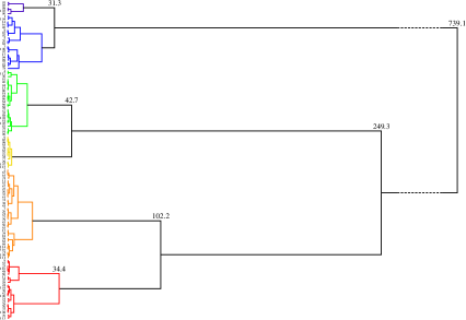
(log-normal index movement model)

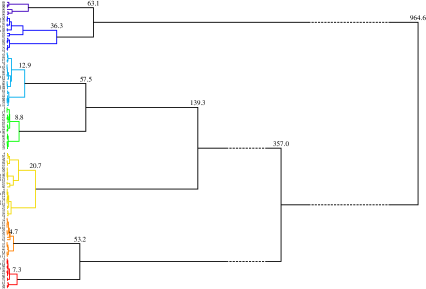
Figure 1: The complete-link hierarchical clustering trees of the segments obtained using the normal index movement model (top) and the log-normal index movement model (bottom). The differentiated clusters are coloured according to their market volatilities: low (deep blue and blue), moderate (cyan and green), high (yellow and orange), and extremely high (red). Also shown at the major branches are the Jensen-Shannon divergence values at which subclusters are merged.

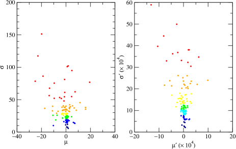
Figure 2: Means and standard deviations of the segments obtained using the normal index movement model (left) and the log-normal index movement model (right). As we can see, the clusters are differentiated primarily by their standard deviations.

When we plot a scatter diagram of the segment means and standard deviations, as shown in Figure 2, we see that the clusters are distinguished primarily through their standard deviations, i.e. their market volatilities. Adopting a heat-map-like colour scheme for the clusters, we colour the low-volatility clusters deep blue and blue, the moderate-volatility clusters cyan and green, the high-volatility clusters yellow and orange, and the extremely-high-volatility clusters red. Using this colour scheme, we plot the temporal distributions of clustered segments for the two models as Figure 3. The two temporal distributions agree qualitatively on the existence of a low-volatility phase between mid-2003 to end-2006, and a high-volatility phase within 2008. However, we find the log-normal index movement model exaggerates small statistical divergences, at the same time playing down large statistical divergences. As such, there is higher temporal contrast at low market volatilities, and lower temporal contrast at high market volatilities. In comparison, the normal index movement model, with its uniform contrast between market volatilities, tells us a much more interesting story: over the period January 1997 to August 2008, the US market, as measured by the DJI, is found predominantly in the low-volatility (deep blue and blue) and high-volatility (yellow and orange) phases. By visual inspection of the DJI time series, we see that the low-volatility phase has a natural interpretation as the economic expansion phase, but while the high-volatility phase contains the economic contraction phase, its duration is significantly longer. From this point on, we will limit our discussions to the normal index movement model.

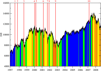
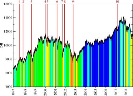
Figure 3: Temporal distributions of the clustered segments for the normal index movement model (top), and the log-normal index movement model (bottom). The red solid lines indicate the dates of important market events: (1) July 1997 Asian Financial Crisis; (2) October 1997 Mini Crash; (3) August 1998 Russian Financial Crisis; (4) DJI 2000 High; (5) NASDAQ Crash; (6) start of 2001 recession; (7) Sep 11 Attack; (8) end of 2001 recession; (9) DJI 2002 Low; (10) February 2007 Chinese Correction.

As we can see from Figure 3, both the low-volatility phase and the high-volatility phase are interrupted by a moderate-volatility market correction phase (green). In the normal index movement model, segments within this phase have very consistent standard deviations of about 20 index points. The length distribution of these market correction segments, however, is bimodal, with one group lasting between 100–200 half-hours (1–2 weeks), and another group lasting between 700–900 half-hours (1.5–2 months). In general, we find more short correction segments within the low-volatility phase, and more long correction segments within the high-volatility phase. The high-volatility phase is also interrupted frequently by an extremely-high-volatility market crash phase, which sports a broad range of standard deviations from 50 to 150 index points. Crash segment lengths were also found to fall into three groups: between 10–40 half-hours (1–3 days), around 100 half-hours (1 week), and between 200–300 half-hours (2–3 weeks).

3.3 Temporal Distribution of Clustered Segments

Most importantly, the temporal distribution of the clustered segments between January 1997 and August 2008 indicates the US market made a transition from the low-volatility phase to the high-volatility phase in mid-1998, went back to the low-volatility phase in mid-2003, and again switched back to the high-volatility phase in mid-2007. The first high-volatility phase observed in this period lasted five years, within which we find not only the official March–November 2001 recession, but also the 2000 high in the DJI. It is generally believed that the DJI 2000 high is the result of the Dot-Com Bubble, even though the March 2000 NASDAQ Crash did not even registered on the DJI. Very interestingly, apart from more or less isolated market corrections, we find a series of market corrections which gets more and more severe prior to the mid-1998 phase transition. We realized that these are precursor shocks similar in nature to those found by Sornette et al preceding market crashes [32, 33, 34, 35]. From Figure 3, we see that the first precursor shock appeared right after the July 1997 Asian Financial Crisis. This suggests, at least on face value, that the mid-1998 transition was triggered by the Asian Financial Crisis. Looking at the end of this first high-volatility phase, we find a series of inverted shocks, starting shortly after the DJI 2002 low. Just like the precursor shocks preceding the low-to-high transition, these low- to moderate-volatily inverted shocks went on for about a year before the US market made the high-to-low phase transition. Though we do not yet understand the nature of these shocks and inverted shocks, it is likely that they are generic features in the dynamics of stock markets.

The second high-volatility phase observed in the DJI time series is none other than the present global financial crisis. Depending on the sources, the Subprime Crisis, which catalyzed the current global financial crisis, is dated as early as July 2007. On the surface, there seems to be no connection between this gradual downturn, and the Feb 2007 market crash known as the Chinese Correction. However, we find the Chinese Correction sitting in the middle of a year-long precursor shock period starting in May 2006, marked by a less severe market event that also had to do with corrections in the Chinese markets. Again, on face value, the US financial crisis appears to be triggered by structural upheavals in a foreign market. However, given that US has substantial investment interests in China, it is not clear from our observations what the true causes and effects might be. Between September 2008 and April 2009, we have yet to detect any inverted shocks, although it is likely the DJI has seen its lowest point of this crisis in March 2009. In the most optimistic scenario that we start finding inverted shocks in April or May 2009, and assuming the fundamental dynamics underlying these entities have not changed from the previous crisis to the present crisis, we can expect the US market to complete the high-to-low phase transition (effectively an economic recovery) in mid-2010.

Finally, after learning so much from the DJI time series, it is natural to ask if it is possible to avert an impending financial crisis, if early detection based on precursor shocks is reliable. To answer such a question, we will need to understand the interplay between factors that caused the precursor shocks. At the very worst, if we cannot understand the nature of these precursor shocks, they would remain useful as early warning indicators of the financial crisis. Our hope then would be that intervention measures meted out early may be able to soften the crisis, and perhaps even shorten it. Equally important, if we can understand what we did in the previous crisis that culminated in the inverted shocks, we might be able to develop more systematic measures to aid recovery from the current crisis.

4 Conclusions

We performed statistical segmentation of the DJI time series between January 1997 and August 2008, using an optimized recursive segmentation scheme derived from that introduced by Bernaola-Galván et al. We assumed normal as well as log-normal index movements in each unknown statistically stationary segment of the time series, and used the Jensen-Shannon divergence as the statistical distance between segments. Adopting the termination heuristic described in Section 2, we found 116 segments for the normal index movement model, and 119 for the log-normal index movement model. These two segmentations agree very well with each other, suggesting that the segment boundaries discovered are statistically robust. We then performed agglomerative hierarchical clustering of the segments using the complete-link algorithm, to find that the large number of segments can be assigned to between five and seven clusters. These clusters are distinguished primarily by their variances, and represent low-volatility, moderate-volatility, high-volatility, and extremely-high-volatility macroeconomic phases.

Based on the temporal distribution of the clustered segments, we saw that the US economy, as measured by the DJI, is found predominantly in the low-volatility phase or the high-volatility phase. The low-volatility phase corresponds very roughly to the economic expansion phase of the standard economic cycle. In contrast, the accepted economic contraction phase is completely nested within the much longer high-volatility phase. Both phases are interrupted frequently by the week-long or month-long moderate-volatility market correction phases. Market crashes, which form a distinct macroeconomic phase with extremely high volatility, occur with durations ranging from one day to three weeks, and is almost exclusively found within the high-volatility phase. Within the period studied, we found the high-volatility occuring only twice. The first such interval was from mid-1998 to mid-2003. The second interval is the ongoing global financial crisis which, according to our results, started in mid-2007.

From the temporal distribution of clustered segments, we found a series of moderate-volatility precursor shocks preceding the mid-1998 low-to-high phase transition, and also a series of moderate-volatility inverted shocks preceding the mid-2003 high-to-low phase transition, which is associated with economic recovery that started with the DJI 2002 low. There is also a series of precursor shocks preceding the mid-2007 low-to-high phase transition that brought many financial giants around the world to their knees. The time scale for all transitions identified from the DJI time series is about a year. We suspect inverted shocks would again appear roughly a year before the end of the current financial crisis. The implication of this finding is that, if we do find inverted shocks trailing the the March 2009 low, and take these as the start of the economic recovery, the US economy might find itself back in the low-volatility phase sometime in the middle of 2010. Should this optimistic scenario pan out, the current high-volatility global financial crisis would have lasted about three years, compared to five years for the previous high-volatility phase.

From the DJI time series data alone, we see at face value that the mid-1998 transition was triggered by the July 1997 Asian Financial Crisis. This assessment runs contrary to most accounts, because the US market actually went on to scale new heights in 2000. However, because of the high volatility between 1998 and 2000, the upward trend within this period must be interpreted very carefully. In comparison, the local trend between 2004 to 2007 is statistically much more significant, because of the low volatility within this period. While the February 2007 market crash known as the Chinese Correction might have played an important role, we see that there are earlier signs for the start of global economic decline in mid-2007. This is an unnamed market event in May 2006, also related to correction within the Chinese markets. All in all, the story that unfolded from our analysis of the DJI time series tells us how the global economies are so coupled to each other, that structural transitions in one market eventually propagates to most markets around the world.

Presently, we have initiated a comparative study of the Nikkei 225 and the DJI over the same period (January 1997 to August 2008), to see whether there are statistical signatures that point to causal links between the US and Japanese markets. At the same time, we are replicating the analysis for the Dow Jones family of US economic sector time series, to search for causal links between different economic sectors. We hope this more extensive analysis will tell us which economic sectors follow which other economic sectors into decline during a financial crisis. We also hope to see which economic sectors lead the economic recovery, and which economic sectors are lifted up by others as the economy recovers. Ultimately, a better understanding of the causal relationships between economic sectors will hint to more effective, and less costly stimulus measures.

References

- [1] National Bureau of Economic Research, “US business cycle expansions and contractions”, http://www.nber.org/cycles.html.
- [2] Wikipedia, “Subprime crisis impact timeline”, http://en.wikipedia.org/wiki/Subprime_crisis_impact_timeline.
- [3] E. G. Carlstein, H.-G. Müller, and D. Siegmund, Change-Point Problems, Lecture Notes-Monograph Series, vol. 23. Institute of Mathematical Statistics, 1994.
- [4] J. Chen and A. K. Gupta, Parametric Statistical Change Point Analysis. Birkhäuser, 2000.
- [5] S. M. Goldfeld and R. E. Quandt, “A Markov Model for Switching Regressions”, Journal of Econometrics, vol. 1, pp. 3–16, 1973.
- [6] J. D. Hamilton, “A New Approach to the Economic Analysis of Nonstationary Time Series and the Business Cycle”, Econometrica, vol. 57, pp. 357-384, 1989.
- [7] C.-J. Kim and C. R. Nelson, “Has the U.S. Economy Become More Stable? A Bayesian Approach Based on a Markov-Switching Model of Business Cycle”, Review of Economics and Statistics, vol. 81, pp. 608-616, 1999.
- [8] Taqtic, SIRCA, https://taqtic.sirca.org.au/TaqTic/.
- [9] J. J. Murphy, Technical Analysis of the Financial Markets, 2nd Edition, New York Institute of Finance, 1999.
- [10] F.-L. Chung, T.-C. Fu, R. Luk, and V. Ng, “Evolutionary Time Series Segmentation for Stock Data Mining”, Proceedings of the IEEE International Conference on Data Mining 2002 (9–12 Dec 2002, Maebashi City, Japan), pp. 83–90, 2002.
- [11] J. Jiang, Z. Zhang, and H. Wang, “A New Segmentation Algorithm to Stock Time Series Based on PIP Approach”, Proceedings of the Third IEEE International Conference on Wireless Communications, Networking and Mobile Computing 2007 (21–25 Sep 2007, Shanghai, China), pp. 5609–5612, 2007.
- [12] J. Xie and W.-Y. Yan, “Pattern-Based Characterization of Time Series”, International Journal of Information and Systems Science, vol. 3, no. 3, pp. 479–491, 2007.
- [13] Z. Zhang, J. Jiang, X. Liu, W. C. Lau, H. Wang, S. Wang, X. Song, and D. Xu, “Pattern Recognition in Stock Data Based on a New Segmentation Algorithm”, Lecture Notes in Computer Science, vol. 14798, pp. 520–525, 2007.
- [14] V. Barranco-López, P. Luque-Escamilla, J. Martínez-Aroza, and R. Román-Roldán, “Entropic Texture-Edge Detection for Image Segmentation”, Electronic Letters, vol. 31, pp. 867–869, 1995.
- [15] J. V. Braun and H.-G. Müller, “Statistical Methods for DNA Sequence Segmentation”, Statistical Science, vol. 13, no. 2, pp. 142–162, 1998.
- [16] P. Bernaola-Galván, P. C. Ivanov, L. A. N. Amaral, and H. E. Stanley, “Scale Invariance in the Nonstationarity of Human Heart Rate”, Physical Review Letters, vol. 87, art. 168105, 2001.
- [17] J. J. Oliver, R. A. Baxter, and C. S. Wallace, “Minimum Message Length Segmentation”, Lecture Notes in Computer Science, vol. 1394, pp. 222-233, 1998.
- [18] D. Lemire, “Overfitting and Time Series Segmentation: A Locally Adaptive Solution”, arXiv:cs/0605103, 2006.
- [19] P. Bernaola-Galván, R. Román-Roldán, and J. L. Oliver, “Compositional Segmentation and Long-Range Fractal Correlations in DNA Sequences”, Physical Review E, vol. 53, no. 5, pp. 5181–5189, 1996.
- [20] R. Román-Roldán, P. Bernaola-Galván, and J. L. Oliver, “Sequence Compositional Complexity of DNA through an Entropic Segmentation Method”, Physical Review Letters, vol. 80, no. 6, pp. 1344–1347, 1998.
- [21] W. Li, “New Stopping Criteria for Segmenting DNA Sequences”, Physical Review Letters, vol. 86, no. 25, pp. 5815–5818, 2001.
- [22] W. Li, “DNA Segmentation as a Model Selection Process”, Proc. Int’l Conf. Research in Computational Molecular Biology (RECOMB), pp. 204–210, 2001.
- [23] S.-A. Cheong, P. Stodghill, D. J. Schneider, S. W. Cartinhour, and C. R. Myers, “Extending the Recursive Jensen-Shannon Segmentation of Biological Sequences”, q-bio/0904.2466.
- [24] S.-A. Cheong, P. Stodghill, D. J. Schneider, S. W. Cartinhour, and C. R. Myers, “The Context Sensitivity Problem in Biological Sequence Segmentation”, q-bio/0904.2668.
- [25] A. Jain, M. Murty, and P. Flynn, “Data Clustering: A Review”, ACM Computing Surveys, 31(3), September 1999.
- [26] J. J. van Wijk and E. R. van Selow, “Cluster and Calendar Based Visualization of Time Series Data”, Proceedings of the 1999 IEEE Symposium on Information Visualization (Oct 24–29, 1999, San Francisco, California, USA), pp. 4–9, 1999.
- [27] A. Krawiecki, J. A. Hołyst, and D. Helbing, “Volatility Clustering and Scaling for Financial Time Series due to Attractor Bubbling”, Phys. Rev. Lett., vol. 89, no. 15, 158701, 2002.
- [28] T. C. Fu, F. L. Chung, R. Luk, and C.-M. Ng, “Financial Time Series Indexing Based on Low Resolution Clustering”, Proceedings of the ICDM 2004 Workshop on Temporal Data Mining: Algorithms, Theory and Applications (Nov 1–4, 2004, Brighton, UK), pp. 4–13, 2004.
- [29] A. R. Admati and P. Pfleiderer, “A Theory of Intraday Patterns: Volume and Price Variability”, The Review of Financial Studies, vol. 1, no. 1, pp. 3–40, 1988.
- [30] C. Gouriéroux, J. Jasiak, and G. Le Fol, “Intra-Day Market Activity”, Journal of Financial Markets, vol. 2, no. 3, pp. 193–226, 1999.
- [31] C. A. Sims and T. Zha, “Were There Regime Switches in U.S. Monetary Policy?”, The American Economic Review, vol. 96, no. 1, pp. 54–81, 2006.
- [32] D. Sornette, A. Johansen, and J.-P. Bouchaud, “Stock Market Crashes, Precursors and Replicas”, J. Phys. I France, vol. 6, pp. 167–175, 1996.
- [33] D. Sornette and A. Johansen, “Large Financial Crashes”, Physica A, vol. 245, pp. 411–422, 1997.
- [34] A. Johansen and D. Sornette, “Modeling the Stock Market Prior to Large Crashes”, The European Physical Journal B, vol. 9, pp. 167–174, 1999.
- [35] A. Johansen, O. Ledoit, and D. Sornette, “Crashes as Critical Points”, International Journal of Theoretical and Applied Finance, vol. 3, no. 2, pp. 219–255, 2000.