On the cavity method for decimated random constraint satisfaction problems and the analysis of belief propagation guided decimation algorithms

Abstract

We introduce a version of the cavity method for diluted mean-field spin models that allows the computation of thermodynamic quantities similar to the Franz-Parisi quenched potential in sparse random graph models. This method is developed in the particular case of partially decimated random constraint satisfaction problems. This allows to develop a theoretical understanding of a class of algorithms for solving constraint satisfaction problems, in which elementary degrees of freedom are sequentially assigned according to the results of a message passing procedure (belief-propagation). We confront this theoretical analysis to the results of extensive numerical simulations.

I Introduction

In constraint satisfaction problems (CSP) a set of variables is required to simultaneously satisfy a series of constraints. One can equivalently define an energy function as the number of unsatisfied constraints of a given assignment of the variables, and rephrase the CSP as the quest for a zero energy groundstate configuration. This analogy with low temperature physics triggered an intensive research effort within the statistical mechanics community. More precisely, one line of approach for these problems consists in looking for typical properties of randomly generated large instances. This translates into the presence of quenched disorder in the corresponding physical model. The constraints to be satisfied are generally contradicting each other, and the definition of the random instances does not involve an underlying finite dimensional space; in consequence these problems fall into the category of mean-field spin glasses, for which a set of analytical tools have been developed during the last decades Beyond ; Talagrand ; IPC .

The most famous example of random CSP is the random $k$-sat ensemble. Statistical mechanics studies have led to two kind of results for this problem. On the one hand, qualitative and quantitative predictions have been made about the various phase transitions encountered for the typical behaviour of large instances when the control parameter governing the amount of frustration is varied. The satisfiability transition marks the sudden disappearance of the solutions (zero-energy groundstates). There exist rigorous results on the properties of this transition Friedgut and bounds lb ; ub on its possible location. Statistical mechanics has complemented these results with an heuristic way to compute this threshold hence yielding quantitative conjectures on its value MeZe ; MePaZe ; MeMeZe . Another important contribution has been the suggestion of other phase transitions in the satisfiable regime, that concerns the geometrical organization of the set of solutions inside the configuration space BiMoWe ; MeZe ; MePaZe ; pnas . For large enough frustration, but below the satisfiability transition, the solutions can be grouped in clusters of nearby solutions, each cluster being separated from the others.

On the other hand attention has also been paid to algorithmic issues, that is to procedures aiming at solving CSP, by finding their solutions or proving that no solution exist. These algorithms can be roughly divided in two broad categories: local search and sequential assignment procedures. In the first one, which has also been studied with statistical mechanics methods wsat1 ; wsat2 ; wsat3 , a random walk is performed in the configuration space, with transition rules tuned to bias the walk towards the solutions. This kind of algorithm is called incomplete: it cannot prove the absence of solution if it fails to find one. The second category proceeds differently: at some step of the algorithm only one part of the variables has a definite value, the others being still free. Each step thus corresponds to the choice of one free variable and of the value it will be assigned to, the CSP on the remaining variables being consequently simplified. The heuristics guiding these choices can be more or less elaborate. In the simplest cases one only takes into account simple properties of the free variables, such as the number of their occurences in the remaining CSP. A rigorous analysis of these simple (“myopic”) approaches is possible and is at the basis of most of the lower bounds on the satisfiability transition lb . Such algorithms can be made complete if backtracking is allowed, i.e. choices which have led to a contradiction can be corrected in a systematic way. This complete version of the procedure is called the DPLL algorithm DPLL .

One outcome of the statistical mechanics studies of random CSP has been the proposal of an incomplete sequential assignment algorithm called Survey Propagation inspired decimation MeZe ; SID , which proved to be very efficient on satisfiable random instances close to the satisfiability transition. This algorithm relies on the clustering picture of the solution space in the satisfiable regime. Unfortunately its theoretical analysis is much more difficult than for myopic ones. Indeed the heuristics of choice of the variables to be assigned is based on the result of a message passing iterative computation which depends on the whole remaining CSP in an intricate way. More generally the analysis of message-passing decimation procedures is difficult and there are few results on this issue, with the notable exception of MosselPlanted ; unif_sat ; unif_sat2 for the so-called Warning Propagation algorithm on overconstrained satisfiability formulas.

In this paper we provide an analytical description of an algorithm similar to Survey Propagation, yet simpler. It has been studied numerically in Pretti ; Aurell . A part of our results were published in allerton , the method developed there was also applied to another family of CSP in ZdMe . In the sequential assignment procedure under investigation the choice of the value of the assigned variable is made at each step according to the Belief Propagation message passing algorithm (instead of Survey Propagation). It aims at mimicking the following ideal procedure. After a certain number of variables has been assigned, one can define the uniform probability measure over the solutions of the CSP which are still compatible with the previous choices. If one were able to compute the marginal probabilities of this (conditional) probability measure and use them to draw the value of the newly assigned variable at each step, one would construct an uniform sampler of the solutions of the original CSP, and this would in particular lead to an algorithm for finding one solution of the CSP. The computation of these marginal probabilities is a computationally intractable task; Belief Propagation is a fast heuristic algorithm, widely used for inference problems factor ; Yedidia , which is often able to compute good approximations of these marginal probabilities. Analyzing the behaviour of the Belief inspired decimation procedure thus amounts to control the error which accumulates at each step by using the BP approximate estimates of the marginal probabilities instead of the exact ones. A theoretical understanding and quantitative description of the deviations between exact and BP-computed marginal probabilities for graphical models is a formidable open problem that we shall not attack directly in this paper. We will instead perform a theoretical analysis of the putative algorithm based on an hypothetic exact marginal computation. This analysis will be obtained by a generalization of the cavity method which is able to deal with the partially decimated CSP encountered along the execution of the algorithm, and to compute the extended phase diagram of these problems. This approach is technically similar to the computation of Franz-Parisi quenched potentials potential . The relevance of this theoretical analysis for the understanding of the approximate BP implementation will then be argued on the basis of a comparison with extensive numerical simulations.

The paper is organized as follows. In Sec. II we give a more precise definition of the ideal decimation procedure sketched above and explain how an approximate realization of this idea can be performed in practice. Sec. III is devoted to the cavity method for decimated formulas that provides an analytical description of the ideal decimation procedure. In the next two sections we apply this formalism to two specific CSP, and compare its predictions to the results of numerical simulations of the BP guided decimation algorithm. We begin in Sec. IV with the xor-satisfiability problem, a well-studied simple example for which many results can be checked with alternative techniques. We then turn to the case of $k$-satisfiability random instances in Sec. V. We draw our conclusions in Sec. VI. More technical details are deferred to an Appendix.

II A thought experiment

II.1 Definition of random CSPs and a brief review of their properties

A Constraint Satisfaction Problem (CSP) is defined on a set of $N$ variables $\sigma_{1},\dots,\sigma_{N}$, taking values in a finite alphabet. We shall denote $\underline{\sigma}=(\sigma_{1},\dots,\sigma_{N})$ the global configuration of the variables, and for a subset $S$ of the indices $\{1,\dots,N\}$ we call $\underline{\sigma}_{S}=\{\sigma_{i},i\in S\}$ the partial configuration of the variables in $S$. The solutions of the CSP are the configurations which simultaneously satisfy $M$ constraints (also called clauses in the following), each of them being specified by a function $\psi_{a}(\underline{\sigma}_{\partial a})$ of a subset $\partial a$ of the variables. The function $\psi_{a}$ takes value 1 (resp. 0) whenever the constraint is satisfied (resp. unsatisfied). A CSP admits a natural representation in terms of a factor graph factor , i.e. a bipartite graph where one type of vertex (variable node) is associated to each variable $i=1,\dots,N$, another type (function node) to each constraint $a=1,\dots,M$. An edge links the $i$’th variable node with the $a$’th function node whenever the constraint $\psi_{a}$ depends on $\sigma_{i}$, i.e. in the notation introduced above whenever $i\in\partial a$. We shall similarly denote $\partial i$ the set of function nodes which depend on the $i$’th variable, and define the distance between two variable nodes $i$ and $j$ as the minimal number of constraint nodes encountered on a path of the factor graph joining $i$ and $j$.

In the following we will concentrate on two examples of CSP, both on binary variables that we shall represent by Ising spins, $\sigma_{i}=\pm 1$:

• $k$-xorsat. Each constraint $a$ depends on $k$ distinct variables $\partial a=\{i_{1}^{a},\dots,i_{k}^{a}\}$, and requires the product of the corresponding spins to take a given value $J^{a}\in\{-1,+1\}$:

  $$\psi_{a}(\underline{\sigma}_{\partial a})=\mathbb{I}\left(\prod_{i\in\partial a}\sigma_{i}=J^{a}\right)\ ,$$ (1)

  where here and in the following $\mathbb{I}(\cdot)$ is the indicator function of an event. This condition is easily seen to be equivalent to a constraint on the value of the eXclusive OR of $k$ boolean variables, hence the name of the problem.

• $k$-sat. The constraint $a$ depends again on $\partial a=\{i_{1}^{a},\dots,i_{k}^{a}\}$, but imposes the configuration of these $k$ variables to avoid one out of the $2^{k}$ possible ones,

  $$\psi_{a}(\underline{\sigma}_{\partial a})=1-\mathbb{I}\left(\sigma_{i}=J_{i}^{a}\ \forall i\in\partial a\right)\ ,$$ (2)

  where $(J_{i_{1}^{a}}^{a},\dots,J_{i_{k}^{a}}^{a})\in\{-1,+1\}^{k}$ are fixed constants defining the constraint. Equivalently, one requires the logical OR of $k$ literals (a boolean variable or its negation) to evaluate to TRUE.

From a computational complexity point of view these two problems are very different. The decision version of a CSP consists in determining whether it admits at least one solution, i.e. one configuration satisfying all constraints simultaneously. The $k$-xorsat decision problem belongs to the easy, polynomial P complexity class NP for any value of $k$. One can indeed use Gaussian elimination to check if the associated system of linear equations modulo 2 is solvable. $k$-sat is on the contrary NP-complete for all $k\geq 3$: no algorithm able to decide the satisfiability of every $k$-sat formula in a time bounded by a polynomial of the formula size is known.

Despite this deep difference in the worst-case point of view, these two families of problems share common features in their “average complexity” behavior. By this we mean the random ensembles of instances that have been extensively studied in the computer science and statistical physics literature and that are defined as follows. A random $k$-xorsat formula is generated by drawing in an independent, identical way $M$ constraints; the $k$-uplet of indices $\partial a$ is drawn uniformly among the $\binom{N}{k}$ possible ones, and the coupling constant $J^{a}$ is taken to be $\pm 1$ with equal probability one half. The generation of a random $k$-sat formula is similar, with for all constraints $a$ the $k$ constants $\{J_{i}^{a}\}_{i\in\partial a}$ being taken independently equal to $\pm 1$ with equal probability. These random ensembles exhibit a rich phenomenology in the thermodynamic limit $N,M\to\infty$ with $\alpha=M/N$ fixed. In particular a satisfiability phase transition occurs at a value $\alpha_{\rm s}$ (which depends on the value of $k$ and on the problem, sat or xorsat, under consideration): random formulas with $\alpha<\alpha_{\rm s}$ are, with high probability, satisfiable, whereas for $\alpha>\alpha_{\rm s}$ they are unsatisfiable. Here and in the following “with high probability” (w.h.p.) means with a probability going to one in the above stated thermodynamic limit. To be more precise, for xorsat this statement has been proven and the values of $\alpha_{\rm s}$ have been computed xor1 ; xor2 . For sat random formulas this satisfiability transition is, strictly speaking, only a conjecture. The existence of a tight threshold $\alpha_{\rm s}(N)$ has been proven in Friedgut , but not the convergence of $\alpha_{\rm s}(N)$, that could in principle oscillate between the bounds on its possible location lb ; ub . It is however most probable that the values of $\alpha_{\rm s}$ computed within the statistical mechanics framework MeZe ; MePaZe ; MeMeZe are exact.

Besides the satisfiability transition other interesting phenomena occurs in the satisfiable phase $\alpha<\alpha_{\rm s}$. In this regime the formula are w.h.p. satisfiable and in fact admits an exponential number of solutions; however there are structural phase transitions at which the properties of the set of solutions change qualitatively. To describe the set of solutions it is convenient to introduce the uniform probability measure on this set,

$$\mu(\underline{\sigma})=\frac{1}{Z}\prod_{a=1}^{M}\psi_{a}(\underline{\sigma}_{\partial a})\ ,$$ (3)

where the normalizing factor $Z$ is the number of solutions of the CSP. Note that this probability measure is itself a random object, as it depends on the instance of the CSP under study, and that it is defined only for the satisfiable instances, which is the case w.h.p. in the regime $\alpha<\alpha_{\rm s}$ we are considering here.

In the xorsat ensemble of random formulas there is a single structural phase transition in the satisfiable regime xor1 ; xor2 , known as the clustering transition with a threshold denoted $\alpha_{\rm d}$. For lower values of the connectivity $\alpha$, the set of solutions is well-connected. On the contrary for $\alpha_{\rm d}<\alpha<\alpha_{\rm s}$ the exponential number of solutions gets splitted in an exponential number $\exp[N\Sigma]$ of clusters, separated from each other in the configuration space. The rate of growth $\Sigma$ of the number of clusters is usually called the complexity, it decreases when $\alpha$ grows and vanishes at the satisfiability threshold. In the clustered phase each cluster contains the same exponential number of solutions (with a rate of growth called internal entropy). The structure of xorsat is sufficiently simple for a clear-cut definition of the clusters to be possible. In fact the clustering transition corresponds to a percolation transition in the associated factor graph, where an extensive 2-core discontinuously appears.

The structure of the satisfiable phase of the random satisfiability ensemble is richer pnas ; sat_long . At the clustering transition BiMoWe ; MeZe the exponentially numerous clusters have, contrarily to xorsat, a large diversity of internal entropies. This leads, for $k\geq 4$, to another transition, the condensation one at $\alpha_{\rm c}$. When $\alpha_{\rm d}<\alpha<\alpha_{\rm c}$ the measure (3) is splitted in an exponential number of clusters, while for $\alpha_{\rm c}<\alpha<\alpha_{\rm s}$ almost all solutions are contained in a sub-exponential number of clusters. These various phase transitions can be characterized in terms of the strength of the correlations between variables. The clustering $\alpha_{\rm d}$ is related to the appearance of long-range point-to-set correlations, or in other words to the possibility of reconstruction of the value of a variable given the values of all the variables at a large distance from it MeMo . At the condensation transition non trivial correlations are already revealed by the correlation functions between a finite number of variables pnas .

II.2 Oracle guided algorithm and ensemble of decimated CSPs

The study presented in this paper is based on the analysis of an ideal procedure to find the solutions of a CSP, that we discuss here more precisely. Consider a satisfiable CSP instance, and the uniform measure $\mu(\cdot)$ over its solutions defined in (3). Let us also introduce a subset $D$ of the variables, and a partial configuration of these variables $\underline{\tau}_{D}$ compatible with at least one solution of the instance. We can thus define a conditional version of $\mu$, $\mu(\cdot|\underline{\tau}_{D})$, which is the uniform measure over the solutions of the formula compatible with $\underline{\tau}_{D}$:

$$\mu(\underline{\sigma}|\underline{\tau}_{D})=\begin{cases}\frac{1}{Z(\underline{\tau}_{D})}\prod_{a=1}^{M}\psi_{a}(\underline{\sigma}_{\partial a})&\text{if}\ \underline{\sigma}_{D}=\underline{\tau}_{D}\\ 0&\text{otherwise}\end{cases}\ .$$ (4)

The normalization $Z(\underline{\tau}_{D})$ counts the number of solutions compatible with the partial assignment of the variables in $D$.

A possible procedure for sampling from $\mu(\cdot)$ goes as follows. Choose arbitrarily a permutation of $\{1,\dots,N\}$, denoted $i(1),\dots,i(N)$, and call $D_{t}=\{i(1),\dots,i(t)\}$ for $t=1,\dots,N$, $D_{0}=\emptyset$. Construct now sequentially a configuration $\underline{\tau}$, assigning at time $t$ the value $\tau_{i(t)}$; to this aim draw $\sigma_{i(t)}$ according to the marginal of the conditioned measure $\mu(\cdot|\underline{\tau}_{D_{t-1}})$, and set $\tau_{i(t)}=\sigma_{i(t)}$. It is easy to see that after $t$ steps of the algorithm the partial configuration $\underline{\tau}_{D_{t}}$ is distributed according to the marginal law of $\mu(\cdot)$. In particular the final configuration $\underline{\tau}$ obtained when the $N$ variables are assigned is a uniformly chosen solution of the CSP.

This simple algorithm would thus provide a uniform sampler of the solution set of any CSP; it is however only meant as a thought experiment. Indeed, computing exactly the probabilities $\mu(\sigma_{i(t)}|\underline{\tau}_{D_{t-1}})$ is in general a $\#$P-complete problem, with no polynomial algorithm known until now, and we shall thus content ourselves with faster yet approximative means for computing these marginal probabilities. Before introducing them let us discuss further the idealized procedure.

The analytical description of the dynamics followed by this ideal process seems very difficult: at each time step the probability of the evolution $\underline{\tau}_{D_{t-1}}\to\underline{\tau}_{D_{t}}$ depends in a non-trivial way on all the choices made in the previous steps. However the description of the process at a given point of its evolution is very simple. As noted above $\underline{\tau}_{D_{t}}$ is distributed according to the marginal of $\mu(\cdot)$. One can state this in a slightly different way: $\underline{\tau}_{D_{t}}$ can be obtained by drawing uniformly a solution $\underline{\tau}$ from $\mu(\cdot)$, retaining the configuration of the variables in $D_{t}$, and discarding the rest of the configuration. We shall further assume that the permutation $i(1),\dots,i(N)$ is drawn uniformly at random, such that $D_{t}$ is a random set of $t$ variables among $N$. In the thermodynamic limit we shall define $\theta=t/N$, the fraction of assigned variables, and consider for simplicity that $D_{\theta N}$ is built by retaining independently each variable with probability $\theta$ (we only make an error of order $1/\sqrt{N}$ on the fraction of variables thus included in $D$).

These considerations lead us to the definition of an ensemble of CSP instances parametrized by $\alpha$ and $\theta$, generalizing the original one which corresponds to $\theta=0$. Explicitly this ensemble of formulas corresponds to the following generation process:

1. draw a satisfiable CSP with parameter $\alpha$

2. draw a uniform solution $\underline{\tau}$ of this CSP

3. choose a set $D$ by retaining each variable independently with probability $\theta$

4. consider the residual formula on the variables outside $D$ obtained by imposing the allowed configurations to coincide with $\underline{\tau}$ on $D$.

Let us emphasize that, apart from simple cases like the xorsat model, these ensembles do not coincide in general with randomly uniform formulas conditioned on their degree distributions. The fact that the generation of the configuration $\underline{\tau}$ depends on the initial CSP induces non-trivial correlations in the structure of the final formula.

We shall see in the following how to adapt the statistical mechanics techniques to compute the typical properties of such generalized formulas, and in particular to determine the phase transition thresholds in the $(\alpha,\theta)$ plane. One characterization of these random ensembles is the quenched average residual entropy,

$$\omega(\theta)=\lim_{N\to\infty}\frac{1}{N}\mathbb{E}_{F}\mathbb{E}_{\underline{\tau}}\mathbb{E}_{D}[\ln Z(\underline{\tau}_{D})]\ ,\qquad Z(\underline{\tau}_{D})=\sum_{\underline{\sigma}}\prod_{a=1}^{M}\psi_{a}(\underline{\sigma}_{\partial a})\,\mathbb{I}(\underline{\sigma}_{D}=\underline{\tau}_{D})\ ,$$ (5)

where the three expectation values correspond to the three steps of the definition above. This quantity is similar, yet distinct, from the Franz-Parisi quenched potential potential . The definition of the latter also involves a “thermalized” reference configuration $\underline{\tau}$, but is given by the free-energy of the measure on the configurations at a given Hamming distance from $\underline{\tau}$. In other words the two real replicas $\underline{\sigma}$ and $\underline{\tau}$ are coupled uniformly across the variables in Franz-Parisi quenched potential, whereas in the definition of $\omega$ they are coupled infinitely strongly on $D$ where they are forced to coincide, and not at all outside $D$. The computations presented in the rest of the paper can however be easily adapted to obtain the usual quenched potential.

We shall characterize the reduced measure $\mu(\cdot|\underline{\tau}_{D})$ more precisely by computing other quantities besides $\omega(\theta)$. The existence of clusters in this measure will be tested by the computation of the long-range point-to-set correlations and the complexity of the typical clusters.

II.3 Bethe-Peierls approximation for decimated CSPs

We recall in this section the Bethe-Peierls approximation for statistical models defined on factor graphs and show how to adapt it to partially decimated CSPs. Let us first consider a probability measure with a weight funcion which can be factorized as in Eq. (3), with $\psi_{a}$ some a priori arbitrary positive functions. The Bethe approximation for the computation of the partition function $Z$ consists in extremizing the following expression,

$$\ln Z=-\sum_{i,a\in\partial i}\ln\left(\sum_{\sigma_{i}}\nu_{a\to i}(\sigma_{i})\eta_{i\to a}(\sigma_{i})\right)+\sum_{a}\ln\left(\sum_{\underline{\sigma}_{\partial a}}\psi_{a}(\underline{\sigma}_{\partial a})\prod_{i\in\partial a}\eta_{i\to a}(\sigma_{i})\right)+\sum_{i}\ln\left(\sum_{\sigma_{i}}\prod_{a\in\partial i}\nu_{a\to i}(\sigma_{i})\right)$$ (6)

over the unknown $\{\nu_{a\to i},\eta_{i\to a}\}$. These are probability measures on the alphabet of $\sigma_{i}$, defined on the directed edges of the factor graph, which we shall call messages for reasons that will become clear below. The extremization of the Bethe approximation for $\ln Z$ leads to a set of equations between the messages,

$$\nu_{a\to i}(\sigma_{i})=f(\{\eta_{j\to a}\}_{j\in\partial a\setminus i})\ ,\qquad\eta_{i\to a}(\sigma_{i})=g(\{\nu_{b\to i}\}_{b\in\partial i\setminus a})\ ,$$ (7)

where the (edge-dependent) functions $f$ and $g$ are defined by

$$\nu_{a\to i}(\sigma_{i})=\frac{1}{z_{a\to i}}\sum_{\underline{\sigma}_{\partial a\setminus i}}\psi_{a}(\underline{\sigma}_{\partial a})\prod_{j\in\partial a\setminus i}\eta_{j\to a}(\sigma_{j})\ ,\qquad\eta_{i\to a}(\sigma_{i})=\frac{1}{z_{i\to a}}\prod_{b\in\partial i\setminus a}\nu_{b\to i}(\sigma_{i})\ ,$$ (8)

with $z_{a\to i}$ and $z_{i\to a}$ ensuring the normalization of $\nu_{a\to i}$ and $\eta_{i\to a}$. When the factor graph is a tree the log partition function is exactly given by (6) evaluated on the unique solution of the stationarity equations (8), see for instance factor . The messages $\nu_{a\to i}$ (resp. $\eta_{i\to a}$) are then the marginal probabilities for $\sigma_{i}$ of a modified measure corresponding to a factor graph where all factor nodes around $i$ except $a$ have been removed (resp. only $a$ has been removed). From the knowledge of the messages solution of (8) one can compute the marginal probability of the variables in the full factor graph law (3), for instance the marginal probability of variable $i$ reads

$$\frac{1}{z_{i}}\prod_{a\in\partial i}\nu_{a\to i}(\sigma_{i})\ ,$$ (9)

with again $z_{i}$ fixed by normalization. In general factor graphs do contain loops, in that case (6,8,9) are only approximations, at the basis of the so-called Belief Propagation algorithm discussed in more details below.

The Bethe approximation can be easily adapted to the case where the configuration is forced to the value $\underline{\tau}_{D}$ on a subset of the sites $i\in D$, that is to the conditional measure (4). The estimation of the conditioned log partition function follows from (6):

$$\ln Z(\underline{\tau}_{D})=-\sum_{i\notin D,a\in\partial i}\ln\left(\sum_{\sigma_{i}}\nu_{a\to i}^{\underline{\tau}_{D}}(\sigma_{i})\eta_{i\to a}^{\underline{\tau}_{D}}(\sigma_{i})\right)+\sum_{a}\ln\left(\sum_{\underline{\sigma}_{\partial a}}\psi_{a}(\underline{\sigma}_{\partial a})\prod_{i\in\partial a}\eta_{i\to a}^{\underline{\tau}_{D}}(\sigma_{i})\right)+\sum_{i\notin D}\ln\left(\sum_{\sigma_{i}}\prod_{a\in\partial i}\nu_{a\to i}^{\underline{\tau}_{D}}(\sigma_{i})\right)\ ,$$ (10)

where the messages $\{\eta_{i\to a}^{\underline{\tau}_{D}},\nu_{a\to i}^{\underline{\tau}_{D}}\}$ depend on the imposed partial configuration $\underline{\tau}_{D}$. They indeed obey the same equations (8), complemented with the boundary conditions $\eta_{i\to a}^{\underline{\tau}_{D}}(\sigma_{i})=\delta_{\sigma_{i},\tau_{i}}$ when $i\in D$.

II.4 Practical approximate implementation of the thought experiment

The ideal sampling algorithm described in Sec. II.2 cannot be practically implemented, because the computation of the marginals of the probability law $\mu(\underline{\sigma}|\underline{\tau}_{D})$ has generically a cost exponential in the number of variables. One can however mimic this procedure, using a faster yet approximate estimation of the marginals of $\mu(\underline{\sigma}|\underline{\tau}_{D})$ by means of the Belief Propagation algorithm. This modification of the ideal sampler, which will be called BP guided decimation in the following, thus corresponds to (for a given CSP instance):

1. choose a random order of the variables, $i(1),\dots,i(N)$, call $D_{0}=\emptyset$, $D_{t}=\{i(1),\dots,i(t)\}$

2. for $t=1,\dots,N$:

   1. find a fixed point of the BP equations (7) with the boundary conditions $\eta_{i\to a}(\sigma_{i})=\delta_{\sigma_{i},\tau_{i}}$ when $i\in D_{t-1}$

   2. draw $\sigma_{i(t)}$ according to the BP estimation of $\mu(\sigma_{i}|\underline{\tau}_{D_{t-1}})$ given in (9)

   3. set $\tau_{i(t)}=\sigma_{i(t)}$

The Belief Propagation part of the algorithm corresponds to step 2.(a). It amounts to search for a stationary point of the Bethe approximation for the log partition function, in an iterative manner. The unknowns of the Bethe expression, $\eta_{i\to a}$ (resp. $\nu_{a\to i}$), are considered as messages passed from a variable to a neighboring clause (resp. from a clause to a variable). In a random sequential order a message, say $\eta_{i\to a}$, updates itself by recomputing its value from the current messages sent by its neighbors $\{\nu_{b\to i}\}_{b\in\partial i\setminus a}$, according to the equation in (8). If the factor graph of the formula were a tree, these iterations would converge in a finite number of updates to the unique fixed point solution of (8). On generic factor graphs there is no guarantee of convergence of these iterations, in practical implementations one has thus to precise the definition of the algorithm, giving criterions to stop the iterations of the BP updates, we shall come back to this point in Sec. V.5.

The definition of the probability measure conditioned on the choice of the reference configuration $\underline{\tau}_{D}$ (4) and the subsequent derivation of the BP equations only make sense if the formula admits at least one solution compatible with $\underline{\tau}_{D}$. In the analysis of the ideal algorithm this is automatically the case as soon as the initial formula is satisfiable. However this can fail in the course of the BP guided decimation algorithm because the marginals used to generate the configuration $\underline{\tau}$ are only approximate. The BP equations are no longer well defined when there are no solutions of the formula compatible with $\underline{\tau}_{D}$. This shows up for instance in the computation of the message sent by a variable $i$ to a clause $a$; whenever the product $\prod_{b\in\partial i\setminus a}\nu_{b\to i}(\sigma_{i})$ vanishes for all possible values of $\sigma_{i}$ the message $\eta_{i\to a}$ can no longer be normalized, a contradiction has occured between the strong requests imposed by the clauses in $\partial i\setminus a$. The BP guided decimation algorithm has then to stop and fails to construct a solution of the formula.

This mechanism which unveils the contradictions in the choice of $\underline{\tau}_{D}$, and the fact that no solution is compatible with it, is actually equivalent to the Unit Clause Propagation (UCP) algorithm well known in computer science. For concreteness let us recall its functioning in the case of satisfiability formulas. UCP takes in input a list of variables and a list of clauses. If all clauses have length greater or equal to 2 it stops. Otherwise it chooses one of the unit clauses (i.e. of length 1). The variable in this unit clause must be fixed to the value satisfying the clause for the constructed configuration of variables to be a solution of the formula. The logical implications of this assignment are then drawn. All the clauses where the fixed variable appeared with the same sign as in the unit clause can be removed from the formula, as they are automatically satisfied. All clauses where it appeared with the opposite sign are effectively reduced in length, as the fixed variable will never satisfy them. This process is iterated as long as unit clauses are present in the formula. If clauses of length 0 are produced during the propagation of logical implications, then the input formula was not satisfiable: the logical implications required at least one of the variables to take simultaneously its two possible values. If no contradictions occur, the set of variables that appeared in unit clauses during the process are termed logically implied, their value being uniquely determined by the input formula.

It turns out that an equivalent formulation of the UCP rule for drawing logical implications can be given in terms of a message passing procedure known as Warning Propagation (WP) SID . The messages $\{\mathfrak{n}_{i\to a},\mathfrak{v}_{a\to i}\}$ that WP sends along edges of the factor graph are projections of those of BP, where the only informations retained is whether a value of the variable $\sigma_{i}$ is authorized ($\eta_{i\to a}(\sigma_{i})>0$) or not ($\eta_{i\to a}(\sigma_{i})=0$):

$$\mathfrak{n}_{i\to a}(\sigma_{i})=\mathbb{I}(\eta_{i\to a}(\sigma_{i})>0)\ ,\qquad\mathfrak{v}_{a\to i}(\sigma_{i})=\mathbb{I}(\nu_{a\to i}(\sigma_{i})>0)\ .$$ (11)

The projection of the BP equations (7) leads to recurrence equations on the WP messages,

$$\mathfrak{v}_{a\to i}=\mathfrak{f}(\{\mathfrak{n}_{j\to a}\}_{j\in\partial a\setminus i})\ ,\qquad\mathfrak{n}_{i\to a}=\mathfrak{g}(\{\mathfrak{v}_{b\to i}\}_{b\in\partial i\setminus a})\ .$$ (12)

Monotonicity arguments can be used to show that these recurrence equations, initialized with the permissive value of the messages $\mathfrak{n}_{i\to a}(\sigma_{i})=1$, converge to a unique fixed point independent on the order of updates of the messages. Moreover this fixed point contains the same information as revealed by UCP: a contradiction occurs in UCP if and only if there is a variable $i$ such that

$$\prod_{a\in\partial i}\mathfrak{v}_{a\to i}(\sigma_{i})=0\ \ \forall\ \sigma_{i}\ .$$ (13)

If no contradiction occurs the set of variables logically implied by UCP corresponds to the variables $i$ such that there is only one authorized value $\sigma_{i}$ for it,

$$\exists\ !\ \sigma_{i}\ :\ \prod_{a\in\partial i}\mathfrak{v}_{a\to i}(\sigma_{i})=1\ .$$ (14)

This correspondance was explicitly shown in the case of satisfiability formulas in allerton . In our practical implementation of the BP guided decimation algorithm we check, after each assignment of a variable $\tau_{i}(t)$, whether a contradiction in the partial configuration $\underline{\tau}_{D_{t}}$ can be detected by UCP/WP. According to the pseudocode above we do not immediately assign the variables which are logically implied by $\underline{\tau}_{D_{t}}$; please note however that this does not modify at all the subsequent steps of the algorithm, as the BP equations effectively take into account the effect of these logical implications. We also emphasize the fact that in general there are variables which can only take one value under the law $\mu(\cdot|\underline{\tau}_{D})$, yet that are not unveiled as logically implied by UCP/WP; if this were the case UCP would always be succesful on any satisfiable formula (and incidentally one would have P=NP), which is of course well known to be wrong.

As a final remark on the BP guided decimation algorithm, let us emphasize another difference with the theoretical analysis. In practice we apply the algorithm to uniformly generated formula of CSP, with $\alpha<\alpha_{\rm s}$, which are typically satisfiable in the thermodynamic limit, but we cannot systematically exclude unsatisfiable instances as in the analysis of the ideal algorithm.

III Analysis of the thought experiment with the cavity method

III.1 Reminder on the usual cavity method

The goal of the cavity method is to compute the typical properties in the thermodynamic limit of graphical models defined on random factor graphs, and in particular the average entropy of the associated random CSP. In the simplest situation, known as the replica symmetric (RS) case, the hypothesis of the method is that the Bethe-Peierls approximation is asymptotically exact for the large random factor graphs of the ensemble considered. For concreteness we explain it in a setting encompassing the $k$-(xor)sat formulas, that is where each of the $M=\alpha N$ constraints imply $k$ randomly chosen variables. The prediction for the average log partition function then follows by averaging (6),

$$\lim_{N\to\infty}\frac{1}{N}\mathbb{E}[\ln Z]= - \alpha k\,\mathbb{E}\left[\ln\left(\sum_{\sigma}\nu(\sigma)\eta(\sigma)\right)\right]$$ (15)

$$+ \alpha\,\mathbb{E}\left[\ln\left(\sum_{\sigma_{1},\dots,\sigma_{k}}\psi(\sigma_{1},\dots,\sigma_{k})\,\eta_{1}(\sigma_{1})\dots\eta_{k}(\sigma_{k})\right)\right]+\mathbb{E}\left[\ln\left(\sum_{\sigma}\nu_{1}(\sigma)\dots\nu_{l}(\sigma)\right)\right]\ .$$

Let us detail the justification and the meaning of the right hand side of this relation. We have first used the translational invariance in the definition of the random ensemble: each term in the sums of Eq. (6) contributes on average in the same way. Moreover we have introduced the random variable $\eta$ (resp. $\nu$), whose distribution can be constructed as follows: drawing a random factor graph, finding the solution of the BP equations (7), picking a random edge $i-a$ of the factor graph, and setting $\eta=\eta_{i\to a}$ (resp. $\nu=\nu_{a\to i}$). The averages in the right hand side of (15) are thus over independent copies of $\eta$ and $\nu$, over the random constraint function $\psi$, and over a Poisson random variable $l$ of mean $\alpha k$. This last quantity is the degree of an uniformly chosen variable inside such a factor graph.

The equations fixing the distributions of the random variables $\eta$ and $\nu$ can be obtained either looking for the stationary points of (15) or interpreting the BP equations (7) in the random graph perspective. Both reasoning leads to the distributional equations

$$\nu\overset{\rm d}{=}f(\eta_{1},\dots,\eta_{k-1})\ ,\qquad\eta\overset{\rm d}{=}g(\nu_{1},\dots,\nu_{l})\ .$$ (16)

These equations have to be interpreted as equalities between distributions of random variables. The $\eta_{i}$ (resp. $\nu_{i}$) are independent copies of the random variable $\eta$ (resp. $\nu$), $l$ is a Poissonian random variable of parameter $\alpha k$, and $f$ and $g$ have been defined in (7,8), $f$ being itself random because of the choice of the constraint function $\psi$.

The RS cavity method is based on the assumption of asymptotic correctness of the Bethe-Peierls approximation, which can be rephrased as the existence of a single pure state (or cluster) in the probability law $\mu$. A complementary statement of the RS method concerns the local description of the law $\mu$. Let us consider an arbitrary variable node $i_{0}$, and its depth $L$ neighborhood, that is the set of variables at graph distance smaller or equal than $L$ from $i_{0}$. In such random graph ensembles this neighborhood is, with high probability, a Galton-Watson random tree with Poissonian offspring of mean $\alpha k$ for the variable nodes (the constraint nodes being of course always of degree $k$). In the RS case the marginal of the law $\mu$ for the variables in this neighborhood converges in distribution to the law of a finite tree of depth $L$, the only effect of the rest of the graph being summarized in a single message $\eta$ acting on the boundary (the depth $L$ variables), drawn independently with the fixed point distribution solution of Eq. (16). In other words the depth $L$ variables would be considered independent if the constraints inside the depth $L$ neighborhood around $i_{0}$ were removed.

In the context of random CSPs the RS assumption is only valid for small values of the density of constraints $\alpha$. When this parameter grows the solution space splits into a large number of pure states (clusters), which induces non-trivial correlations between the variables of the graphical model. The cavity method at the level of the first step of replica symmetry breaking (1RSB) is able to describe this situation MePa . Let us sketch some of its important features without entering into technical details. The assumption of the 1RSB method is that the Bethe-Peierls approximation can still be used, but only for the probability measures restricted to a single pure state; to each such pure state is associated a solution of the BP equations (7). In order to handle the proliferation of pure states one introduces, on each directed edge of a given factor graph, a probability distribution, with respect to the choice of the pure states, of the corresponding BP messages. The 1RSB equations linking these distributions on adjacent edges depend on the Parisi parameter $m$, which controls the relative importance of the pure states in the sampling of the corresponding BP messages, according to their internal sizes. A slightly more explicit interpretation of the 1RSB equations has been given in pnas ; sat_long . There it was shown that the distribution over pure states can be viewed as a distribution over ’far-away’ boundary conditions, with a specific probability measure over these boundary conditions depending on $m$. A special role is played by the value $m=1$. In this case the ’far-away’ boundary conditions are themselves drawn from the original Gibbs measure. The clustering transition, that is the appearance of a non-trivial solution of the 1RSB equations at $m=1$, can thus be related to the existence of long-range correlations of a particular type (so called point-to-set) in the Gibbs measure, as first discussed in MeMo . These correlations measure the influence on a variable $i_{0}$ of fixing a subset $B$ of variables, for instance $B(i_{0},\ell)$ the set of variables at distance exactly $\ell$ from $i_{0}$, to a reference value drawn from the equilibrium probability measure. Using the notation of conditional probability defined in Eq. (4) the typical long range point-to-set correlation reads

$$C_{\infty}=\lim_{\ell\to\infty}\lim_{N\to\infty}\mathbb{E}\sum_{\sigma_{i_{0}}}|\mu(\sigma_{i_{0}}|\underline{\tau}_{B(i_{0},\ell)})-\mu(\sigma_{i_{0}})|\ ,$$ (17)

where the expectation is over the equilibrium configuration $\underline{\tau}$ and the factor graph model. In an unclustered regime the influence of the distant boundary vanishes, $C_{\infty}=0$, while in the presence of clustering $C_{\infty}>0$. In the latter case one can moreover compute the complexity of relevant clusters, that is the logarithm of the degeneracy of the clusters which bears the vast majority of the weights of the probability measures (at the leading exponential precision) by computing the difference in entropy of the conditional and original measures, $\mu(\cdot|\underline{\tau}_{B(i_{0},\ell)})$ and $\mu(\cdot)$. The so-called condensation transition is signalled by a vanishing of this complexity. We shall come back in the next subsection on the technical details of the 1RSB $m=1$ computations, generalizing it to the case of partially decimated formulas.

III.2 Cavity method for decimated CSP

We turn now to the extension of the cavity method to partially decimated factor graphs. Our goal is to compute the residual entropy (5) by averaging the Bethe expression (10) with respect to the distribution of the conditional messages $\{\eta_{i\to a}^{\underline{\tau}_{D}},\nu_{a\to i}^{\underline{\tau}_{D}}\}$. The randomness of these objects has several origins: (i) the choice of the factor graph (ii) the generation of the reference configuration $\underline{\tau}$ from the uniform measure $\mu$ (iii) the selection of the decimated variables in $D$, each independently with probability $\theta$. The difficulty of this computation arises from the correlation between (i) and (ii), the measure $\mu$ being itself defined in terms of the factor graph. This dependence can however be handled within the context of the cavity method. Let us suppose indeed that the local properties of the original measure $\mu(\cdot)$ are well described by the assumptions of replica symmetry, that is for $\alpha<\alpha_{\rm c}$. We can thus perform the computation in the random tree model that corresponds locally to the random graph one. In this case the generation of the reference configuration $\underline{\tau}$ of a tree factor graph model can be done recursively, in a broadcasting way, thanks to the Markov property of such probability laws. The value of the root $\tau_{i_{0}}$ is first drawn with its marginal probability computed from the incoming messages according to (9). Then the configuration of the neighbors of $i_{0}$ can be drawn conditioned on the value of $\tau_{i_{0}}$, and the process can be iterated away from the root. Once the reference configuration $\underline{\tau}$ has been generated in such a way, the messages $\{\eta_{i\to a}^{\underline{\tau}_{D}},\nu_{a\to i}^{\underline{\tau}_{D}}\}$ can be computed, their dependence on $\underline{\tau}$ arising from the condition $\eta_{i\to a}^{\underline{\tau}_{D}}(\sigma_{i})=\delta_{\sigma_{i},\tau_{i}}$ for variables $i$ in the decimated set $D$. At this point, for a given tree, reference configuration $\underline{\tau}$ and set $D$, each directed edge of the factor graph bears a pair of messages, for instance $(\nu_{a\to i},\nu_{a\to i}^{\underline{\tau}_{D}})$ on the edge from constraint $a$ to variable $i$. We can now define the random variable $(\nu,\nu^{\tau})_{\ell}$ which has the distribution of $(\nu_{a\to i},\nu_{a\to i}^{\underline{\tau}_{D}})$ when one takes into account the randomness in the choice of the tree, of the set $D$ and of the reference configuration $\underline{\tau}$, the latter being conditioned on $\tau_{i}=\tau$. Moreover the positive integer $\ell$ indexes the depth of the random tree construction. We shall also introduce random variables having the same distribution as $(\eta_{i\to a},\eta_{i\to a}^{\underline{\tau}_{D}})$. For the sake of clarity in the following we actually introduce two versions of these random variables, $(\eta,\eta^{\tau})_{\ell}$ and $(\eta,\widetilde{\eta}^{\,\tau})_{\ell}$, the former being additionally conditioned on $i\notin D$. The equations defining these random variables by recurrence on $\ell$ can now easily be written,

$$(\eta,\widetilde{\eta}^{\,\tau})_{\ell}\overset{\rm d}{=}\begin{cases}(\eta,\eta^{\tau})_{\ell}&\text{with probability}\ 1-\theta\\ (\eta,\delta^{\tau})&\text{otherwise}\end{cases}\ ,$$ (18)

where we defined $\delta^{\tau}(\sigma)=\delta_{\tau,\sigma}$, and

$$(\eta,\eta^{\tau})_{\ell}\overset{\rm d}{=}(g(\nu_{1},\dots,\nu_{l}),g(\nu_{1}^{\tau},\dots,\nu_{l}^{\tau}))\ ,$$ (19)

where $l$ is a Poisson random variable of parameter $\alpha k$ and $(\nu_{1},\nu_{1}^{\tau}),\dots,(\nu_{l},\nu_{l}^{\tau})$ are independent copies of $(\nu,\nu^{\tau})_{\ell}$. Finally one has

$$(\nu,\nu^{\tau})_{\ell+1}\overset{\rm d}{=}(f(\eta_{1},\dots,\eta_{k-1}),f(\widetilde{\eta}_{1}^{\,\tau_{1}},\dots,\widetilde{\eta}_{k-1}^{\,\tau_{k-1}}))\ ,$$ (20)

where the $(\eta_{i},\widetilde{\eta}_{i}^{\,\tau_{i}})$ are independent copies of $(\eta,\widetilde{\eta}^{\,\tau_{i}})_{\ell}$, and the configuration $\tau_{1},\dots,\tau_{k-1}$ is drawn according to

$$P[\tau_{1},\dots,\tau_{k-1}|\tau]=\frac{1}{z}\psi(\tau,\tau_{1},\dots,\tau_{k-1})\eta_{1}(\tau_{1})\dots\eta_{k-1}(\tau_{k-1})\ .$$ (21)

Let us emphasize that the function $\psi$ used in the broadcasting generation of $\tau_{1},\dots,\tau_{k-1}$ is the same (random) constraint function as the one used to compute $f$ in (20), and that the messages $\eta_{i}$ are the same in (20) and (21). We shall discuss a numerical procedure for solving these equations on the example of satisfiability formulas in Sec. V. The prediction of the cavity method for the average residual entropy (5) can finally be expressed in terms of these random variables,

$$\omega= - \alpha k(1-\theta)\,\mathbb{E}\left[\sum_{\tau}\frac{\nu(\tau)\eta(\tau)}{\sum_{\tau^{\prime}}\nu(\tau^{\prime})\eta(\tau^{\prime})}\ln\left(\sum_{\sigma}\nu^{\tau}(\sigma)\eta^{\tau}(\sigma)\right)\right]$$ (22)

$$+ \alpha\,\mathbb{E}\left[\sum_{\tau_{1},\dots,\tau_{k}}\frac{\psi(\tau_{1},\dots,\tau_{k})\eta_{1}(\tau_{1})\dots\eta_{k}(\tau_{k})}{\sum_{\tau^{\prime}_{1},\dots,\tau^{\prime}_{k}}\psi(\tau^{\prime}_{1},\dots,\tau^{\prime}_{k})\eta_{1}(\tau^{\prime}_{1})\dots\eta_{k}(\tau^{\prime}_{k})}\ln\left(\sum_{\sigma_{1},\dots,\sigma_{k}}\psi(\sigma_{1},\dots,\sigma_{k})\widetilde{\eta}_{1}^{\,\tau_{1}}(\sigma_{1})\dots\widetilde{\eta}_{k}^{\,\tau_{k}}(\sigma_{k})\right)\right]$$

$$+ (1-\theta)\,\mathbb{E}\left[\sum_{\tau}\frac{\nu_{1}(\tau)\dots\nu_{l}(\tau)}{\sum_{\tau^{\prime}}\nu_{1}(\tau^{\prime})\dots\nu_{l}(\tau^{\prime})}\ln\left(\sum_{\sigma}\nu_{1}^{\tau}(\sigma)\dots\nu_{l}^{\tau}(\sigma)\right)\right]\ ,$$

where as before $l$ is a Poisson random variable of parameter $\alpha k$ and the various $(\eta_{i},\eta_{i}^{\tau_{i}})$ are independent copies of the corresponding random variables, with the $\ell\to\infty$ limit kept understood.

We shall now discuss an important issue that we kept under silence, namely the definition of the initial condition $(\eta,\eta^{\tau})_{\ell=0}$. Let us first make the connection between the computation just presented and the $m=1$ 1RSB description of non-decimated formulas, that is consider for a while the case $\theta=0$. We shall call $I_{0}$ the initial condition $(\eta,\eta^{\tau})_{\ell=0}\overset{\rm d}{=}(\eta,\eta)$, with $\eta$ a random variable solution of the RS fixed point equation (16). It is easy to show that with such an initial condition $(\eta,\eta^{\tau})_{\ell}\overset{\rm d}{=}(\eta,\eta)$ for all values of $\ell$, and that (22) reduces to the RS prediction (15) for the average entropy. If on the contrary one considers the initial condition $I_{1}$ defined by $(\eta,\eta^{\tau})_{\ell=0}\overset{\rm d}{=}(\eta,\delta^{\tau})$ and iterates the recursion equations (18,19,20), one reproduces the $m=1$ computations in the form of MeMo ; sat_long . This should not be a surprise : the interpretation of the $m=1$ 1RSB formalism presented above was precisely the study of the effect of a far away boundary, which is implemented here in this initial condition and in the limit $\ell\to\infty$. In an unclustered phase the two initial conditions lead to the same random variable $(\eta,\eta)$ in the large $\ell$ limit, the effect of the far away boundary vanishes at long distance and the correlation function (17) is equal to 0. If on the contrary the two initial conditions do not lead to the same limit when $\ell$ diverges the correlation function remains positive, signaling the presence of clustering in the solution space. In that case the value of (22) computed with the initial condition $I_{1}$ is the internal entropy of the relevant clusters, the difference between (15) and (22) is ascribed to the complexity, the degeneracy of the relevant clusters. We now come back to the decimated case $\theta>0$. The two initial conditions are still relevant and have the same interpretation with the measure $\mu(\cdot)$ replaced by $\mu(\cdot|\underline{\tau}_{D})$. Suppose indeed that the point-to-set correlation criterion were to be tested for the typical properties of $\mu(\cdot|\underline{\tau}_{D})$. Then one would compute the generalization of (17),

$$C_{\infty}(\theta)=\lim_{\ell\to\infty}\lim_{N\to\infty}\mathbb{E}\sum_{\sigma_{i_{0}}}|\mu(\sigma_{i_{0}}|\underline{\tau}_{D\cup B(i_{0},\ell)})-\mu(\sigma_{i_{0}}|\underline{\tau}_{D})|\ ,$$ (23)

where the expectation would include an average over the set $D$ of $\theta N$ variables. This is precisely what is realized by the two initial conditions followed by the recursion relations (18,19,20) for this value of $\theta$. Again we shall conclude on the absence of clustering in $\mu(\cdot|\underline{\tau}_{D})$ when the two initial conditions have the same $\ell\to\infty$ limit, and obtain the typical complexity of the clusters from the difference in the values of (22) for the two different initial conditions.

III.3 The cavity computation of the average number of logically implied variables

Another quantity which can be interesting to compute is the amount of logical implications, in the UCP/WP sense explained in Sec. II.4, induced by the choice of the partial reference solution $\underline{\tau}_{D}$. Let us define as

$$\phi(\theta)=\theta+\lim_{N\to\infty}\frac{1}{N}\mathbb{E}_{F}\mathbb{E}_{\underline{\tau}}\mathbb{E}_{D}[\text{nb. directly implied variables}]\ ,$$ (24)

the average fraction of variables which have been explicitly assigned or which can be logically deduced from these assignments. A motivation for the study of this quantity, as explained in allerton , is that $\frac{{\rm d}\phi}{{\rm d}\theta}-1$ is the average number of the newly implied variables as a single assignment step is performed. The size of this set of variables, and in particular its possible divergence with the formula size when $\phi(\theta)$ is discontinuous, should thus be a measure of the sensitivity of the decimation procedure with respects to small errors made by the BP version of the procedure with respects to the ideal one.

The computation of $\phi(\theta)$ can be performed, within the RS assumptions on the local structure of the probability law $\mu(\cdot)$, in the locally equivalent random tree model. For a generic CSP one can reproduce the reasoning above, replacing the conditional messages $\eta_{i\to a}^{\underline{\tau}_{D}}$ by their WP counterparts $\mathfrak{n}_{i\to a}^{\underline{\tau}_{D}}$ according to the projection defined in (11). This leads to the similar definition of sequences of random pairs of variables, $(\eta,\widetilde{\mathfrak{n}}^{\tau})_{\ell}$, $(\eta,\mathfrak{n}^{\tau})_{\ell}$ and $(\eta,\mathfrak{v}^{\tau})_{\ell}$, which obeys recursion equations analogous to Eqs. (18,19,20),

$$(\eta,\widetilde{\mathfrak{n}}^{\tau})_{\ell}\overset{\rm d}{=}\begin{cases}(\eta,\mathfrak{n}^{\tau})_{\ell}&\text{with probability}\ 1-\theta\\ (\eta,\delta^{\tau})&\text{otherwise}\end{cases}\ ,\qquad(\eta,\mathfrak{n}^{\tau})_{\ell}\overset{\rm d}{=}(g(\nu_{1},\dots,\nu_{l}),\mathfrak{g}(\mathfrak{v}_{1}^{\tau},\dots,\mathfrak{v}_{l}^{\tau}))\ ,$$ (25)

$$(\nu,\mathfrak{v}^{\tau})_{\ell+1}\overset{\rm d}{=}(f(\eta_{1},\dots,\eta_{k-1}),\mathfrak{f}(\widetilde{\mathfrak{n}}_{1}^{\tau_{1}},\dots,\widetilde{\mathfrak{n}}_{k-1}^{\tau_{k-1}}))\ .$$ (26)

The function $\phi(\theta)$ can then be computed as

$$\phi(\theta)=\mathbb{E}\left[\sum_{\tau}\eta(\tau)\mathbb{I}(\widetilde{\mathfrak{n}}^{\tau}=\delta^{\tau})\right]\ ,$$ (27)

in the $\ell\to\infty$ limit. This form of the computation is valid for any CSP; in some particular cases one can however devise a more efficient (and numerically more precise) formulation, using the specific form of the constraints rules to replace the WP message in the second entry of the random pair by a probability of implication. We refer the reader to allerton for further details on this computation for random satisfiability formulas.

IV Application to the XORSAT ensemble

We apply in this section the general formalism developed above to the ensemble of xor-satisfiability formulas. As we shall see great simplifications occur for this simple model, and the study of both the decimated ensemble of random formulas and of the BP guided decimation algorithm can in fact be performed with simpler methods xor1 ; xor2 ; xor3 . It is however an instructive toy model to begin with before handling the more involved case of satisfiability formulas, and has deep connections with information theory, in particular with the Low Density Parity Check codes. The analysis of the “Maxwell decoder” in Maxwell is actually very tightly related with the content of this section.

IV.1 BP equations

The constraints of a xorsat CSP have been defined in Eq. (1). The set of solutions of such a CSP exhibits some simplifying symmetries, even in the decimated case where some variables are fixed to a given value. It is indeed easy to realize that a non-decimated variable is either fixed to +1 in all the solutions, or fixed to -1, otherwise it takes the value +1 in exactly half of the solutions and -1 in the other half. Consequently the BP messages $\nu_{a\to i}$ and $\eta_{i\to a}$ can be restricted to a set of three possible types, that we shall encode with three-valued numbers $u_{a\to i}$ and $h_{i\to a}$ according to the following correspondence:

$$\nu_{a\to i}(\sigma_{i})=\begin{cases}\delta_{\sigma_{i},+1}&\Leftrightarrow u_{a\to i}=1\\ \delta_{\sigma_{i},-1}&\Leftrightarrow u_{a\to i}=-1\\ \frac{1}{2}&\Leftrightarrow u_{a\to i}=0\end{cases}\ ,\qquad\eta_{i\to a}(\sigma_{i})=\begin{cases}\delta_{\sigma_{i},+1}&\Leftrightarrow h_{i\to a}=1\\ \delta_{\sigma_{i},-1}&\Leftrightarrow h_{i\to a}=-1\\ \frac{1}{2}&\Leftrightarrow h_{i\to a}=0\end{cases}\ .$$ (28)

With these notations the BP equations (8) can be rewritten as

$$u_{a\to i}=J_{a}\prod_{j\in\partial a\setminus i}h_{j\to a}\ ,\qquad h_{i\to a}=\begin{cases}0&\text{if}\ u_{b\to i}=0\ \ \ \forall b\in\partial i\setminus a\\ +1&\text{if}\ \exists b\in\partial i\setminus a\ \text{with}\ u_{b\to i}=1\\ -1&\text{if}\ \exists b\in\partial i\setminus a\ \text{with}\ u_{b\to i}=-1\end{cases}\ .$$ (29)

The second expression is well defined as long as no contradictions are detected, which means that the conditions in the last two lines are not fulfilled simultaneously. The boundary condition for a decimated variable $i\in D$ is $h_{i\to a}^{\underline{\tau}_{D}}=\tau_{i}$ for all neighboring interactions $a\in\partial i$.

Due to the symmetry of the model the BP equations (29) can actually be regarded as WP equations that express the simplifications of the Unit Propagation rule. The first equation reflects the fact that a constraint imposes the value of one of its variables if and only if the $k-1$ other variables are fixed (either by decimation or by propagation of logical implications), the second means that a variable is fixed as soon as one of its neighboring clauses imposes its value.

IV.2 The cavity method computations

Following the general formalism introduced in Sec. III for the treatment of decimated CSPs and the parametrization of the BP messages in terms of $u$ and $h$, we have to find the distributions of the random variables $(h,h^{\tau})_{\ell}$, $(u,u^{\tau})_{\ell}$ and $(h,\widetilde{h}^{\tau})_{\ell}$ for $\tau=\pm 1$. These are the solutions of Eqs. (18,19,20) specialized to the functions $f$, $g$ and $\psi$ of the xorsat model. The relevant solution of this equation takes a particularly simple form which allows for an analytic solution. The results of xor1 ; xor2 imply indeed that the set of solutions of a non-decimated $k$-xorsat formulas is described by the trivial solution of the RS equation, $u=h=0$. Moreover the value of the conditional message $h^{\tau}$ cannot be equal to $-\tau$ : by definition $h^{\tau}$ describes the measure where the reference solution has been drawn conditional on its value at the root being $\tau$, whereas $h^{\tau}=-\tau$ would mean that all solutions compatible with the values of the reference on some subset of variables $D$ have $-\tau$ at the root, which is in contradiction with the hypothesis. In consequence the solution of (18,19,20) can be looked for under the form:

$$(h,h^{\tau})_{\ell}\overset{\rm d}{=}\begin{cases}(0,0)&\text{with probability}\ 1-x_{\ell}\\ (0,\tau)&\text{with probability}\ x_{\ell}\end{cases}\ ,(u,u^{\tau})_{\ell}\overset{\rm d}{=}\begin{cases}(0,0)&\text{w.p.}\ 1-y_{\ell}\\ (0,\tau)&\text{w.p.}\ y_{\ell}\end{cases}\ ,(h,\widetilde{h}^{\tau})_{\ell}\overset{\rm d}{=}\begin{cases}(0,0)&\text{w.p.}\ 1-\phi_{\ell}\\ (0,\tau)&\text{w.p.}\ \phi_{\ell}\end{cases}\ .$$ (30)

Inserting these forms in (18,19,20) leads to the following equations :

$$\phi_{\ell}=\theta+(1-\theta)x_{\ell}\ ,\qquad x_{\ell}=1-\exp[-\alpha ky_{\ell}]\ ,\qquad y_{\ell+1}=\phi_{\ell}^{k-1}\ ,$$ (31)

which can be closed under a single recursion equation on $\phi_{\ell}$,

$$\phi_{\ell+1}=\theta+(1-\theta)\left(1-e^{-\alpha k\phi_{\ell}^{k-1}}\right)\ .$$ (32)

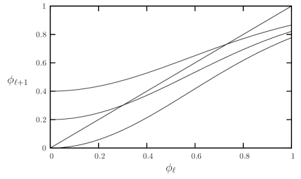
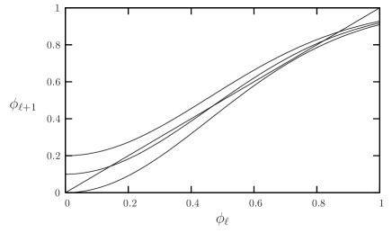
Figure 1: Illustration of the recurrence equation (32) for 3-xorsat. Left panel: $\alpha=0.5<\alpha_{*}(k=3)=2/3$, right panel: $\alpha=0.8>\alpha_{*}$. On each of the plot the three curves are for different values of $\theta$ (growing from bottom to top).

The fixed point equation $\phi_{\ell+1}=\phi_{\ell}$ has between one and three distinct solutions on $[0,1]$, depending on the values of $\alpha$ and $\theta$ (examples of the various situations are provided on Fig. 1). A quick analysis of the equation shows that for $\alpha<\alpha_{*}$, with

$$\alpha_{*}=\frac{1}{k}\left(\frac{k-1}{k-2}\right)^{k-2}\ ,$$ (33)

the equation (32) admits a single solution for all values of $\theta$. If on the contrary $\alpha>\alpha_{*}$, there exists a range of $\theta$, denoted $[\theta_{-}(\alpha),\theta_{+}(\alpha)]$, where Eq. (32) admits three solutions in $[0,1]$. In that case we shall call $\phi(\theta)$ (resp. $\psi(\theta)$) the smallest (resp. the largest) of these three solutions. Some examples of these curves are shown in Fig. 2, and the lines $\theta_{\pm}(\alpha)$ are displayed in Fig. 3.

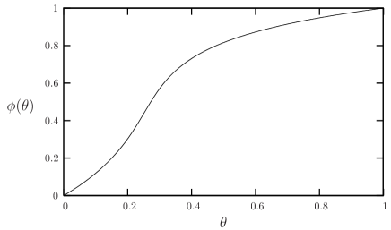
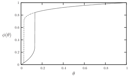
Figure 2: Fixed point solution(s) of Eq. (32) for $k=3$. Left panel: $\alpha=0.5<\alpha_{*}(k=3)=2/3$, right panel: $\alpha=0.8>\alpha_{*}$. The solid line is $\phi(\theta)$, the dashed line in the right panel is $\psi(\theta)$, the largest fixed point solution of Eq. (32).

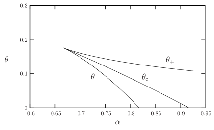
Figure 3: Phase diagram in the $(\alpha,\theta)$ plane for the ensemble of 3-xorsat decimated random formulas, the three critical lines meet at $\alpha_{*}(k=3)=2/3$.

The expression of $\omega$ given in Eq. (22) can be computed using the ansatz (30),

$$\omega=(\ln 2)[\alpha k(1-\theta)(1-xy)-\alpha(1-\phi^{k})-(1-\theta)((\alpha k)(1-y)-\exp[-\alpha ky])]\ ,$$ (34)

where the limit $\ell\to\infty$ is kept understood. Using the relations between $x$, $y$ and $\phi$ stated in (31), one can express this residual entropy in terms of $\phi$,

$$\widehat{\omega}(\phi)=(\ln 2)[1-\phi-\alpha+\alpha k(1-\phi)\phi^{k-1}+\alpha\phi^{k}]\ .$$ (35)

When $\alpha<\alpha_{*}$ the fixed point solution of (32) is unique, hence $\omega(\theta)=\widehat{\omega}(\phi(\theta))$ is a smoothly decreasing function of $\theta$, as plotted on the left panel of Fig. 4. For larger values of $\alpha$, i.e. $\alpha>\alpha_{*}$, we have seen above that there exists a range of parameter $\theta\in[\theta_{-}(\alpha),\theta_{+}(\alpha)]$ where two solutions of (32), $\phi(\theta)$ and $\psi(\theta)$, coexists. On the right panel of Fig. 4 one can see that the two branches of the entropy, $\widehat{\omega}(\phi(\theta))$ and $\widehat{\omega}(\psi(\theta))$ cross each other at an intermediate value $\theta_{\rm c}(\alpha)\in[\theta_{-}(\alpha),\theta_{+}(\alpha)]$, which is also plotted in function of $\alpha$ in the phase diagram Fig. 3. It is natural (and we shall argue in the following that it is the correct choice) to consider that in the region of coexistence the relevant branch is the one leading to the largest entropy, $\omega(\theta)=\max[\widehat{\omega}(\phi(\theta)),\widehat{\omega}(\psi(\theta))]$, which thus exhibits a discontinuity in its slope when $\theta$ crosses $\theta_{\rm c}$.

A direct justification of this choice will be given in the next subsection, here we argue in its favour on the basis of the cavity method. The two boundary conditions discussed in Sec. III.2 corresponds to $\phi_{\ell=0}=0$ ($I_{0}$) and $\phi_{\ell=0}=1$ ($I_{1}$). When the fixed point solution of (32) is unique both initial conditions lead to the same limit $\phi(\theta)$ in the large $\ell$ limit, which leads to the conclusion that there is no clustering in the solution space of the decimated formula for these values of $\alpha$ and $\theta$.

In the region of coexistence these two initial conditions yield, respectively, $\phi_{\ell}\to\phi(\theta)$ and $\phi_{\ell}\to\psi(\theta)$ as $\ell$ diverges. One is thus led to assign the difference $\widehat{\omega}(\phi(\theta))-\widehat{\omega}(\psi(\theta))$ to the complexity of the decimated formula, that is the contribution of the entropy due to the presence of clusters in the measure $\mu(\cdot|D_{\theta N})$. This interpretation is valid only when the complexity is positive, that is in the range $[\theta_{-},\theta_{\rm c}]$. A condensation transition occurs when the threshold $\theta_{\rm c}$ is crossed. In the region $[\theta_{\rm c},\theta_{+}]$ only a subextensive number of clusters are relevant, and the total entropy is equal to their internal entropy. The latter being given by the thermodynamic computation with the initial condition $I_{1}$, one concludes that $\omega(\theta)=\widehat{\omega}(\psi(\theta))$ for $\theta\in[\theta_{\rm c},\theta_{+}]$.

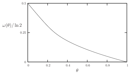
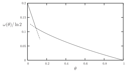
Figure 4: Residual entropy $\omega(\theta)$ for 3-xorsat. Left panel: $\alpha=0.5$, right panel: $\alpha=0.8$. The solid line is the true entropy $\omega(\theta)=\max[\widehat{\omega}(\phi(\theta)),\widehat{\omega}(\psi(\theta))]$, the dashed lines are the two irrelevant branches, $\min[\widehat{\omega}(\phi(\theta)),\widehat{\omega}(\psi(\theta))]$.

IV.3 A more direct computation and its interpretation

It is instructive to rederive the above results on xor-satisfiability decimated formulas by more direct means. Let us first show that for this computation one can assume that the formula is unfrustrated (i.e. $J_{a}=1$ for all constraints) and that in the reference solution $\underline{\tau}$ all variables are fixed to $\tau_{i}=1$. Suppose indeed that the formula has been generated with random $J_{a}=\pm 1$. As we have conditioned the ensemble of formulas on satisfiable ones, there is at least one solution, call it $\underline{\sigma}^{(0)}$. By the gauge transformation $\sigma_{i}\leftrightarrow\sigma^{\prime}_{i}=\sigma_{i}\sigma_{i}^{(0)}$, the solutions $\underline{\sigma}$ of the original problem are in bijection with the solutions $\underline{\sigma}^{\prime}$ of the unfrustrated model. Consider furthermore a reference solution $\underline{\tau}$ of the unfrustrated model and a set $D$ of variables, such that the decimated problem to solve reads

$$\prod_{i\in\partial a}\sigma^{\prime}_{i}=1\ \ \ \forall a\ ,\qquad\sigma^{\prime}_{i}=\tau_{i}\ \ \ \forall i\in D\ .$$ (36)

Applying now the gauge transformation $\sigma^{\prime}_{i}\leftrightarrow\sigma^{\prime\prime}_{i}=\sigma^{\prime}_{i}\tau_{i}$, noting that $\underline{\tau}$ is a solution of the unfrustrated model, one reduces the problem to

$$\prod_{i\in\partial a}\sigma^{\prime\prime}_{i}=1\ \ \ \forall a\ ,\qquad\sigma^{\prime\prime}_{i}=1\ \ \ \forall i\in D\ .$$ (37)

Having get rid of the signs in the constraints and in the reference solution, the size and the structure of the set of solutions of the decimated problem can be deduced from the underlying hypergraph of constraints xor1 ; xor2 ; xor3 .

The initial hypergraph is drawn uniformly with $\alpha N$ clauses of length $k$ among $N$ variables. A fraction $\theta$ of the variables are fixed to +1, and can thus be eliminated from the constraints which are reduced in size. Unit Clause Propagation can then be run to propagate these simplifications. The details of this computation are deferred to Appendix A, we only quote here the results. When UCP stops, there are $N(1-\phi(\theta))$ variables unassigned, with $\phi(\theta)$ the smallest fixed point solution of (32). The simplified formula contains constraints of all lengths $\kappa\in[2,k]$, more precisely there are $\alpha N\binom{k}{\kappa}(1-\phi)^{\kappa}\phi^{k-\kappa}$ clauses of length $\kappa$. The unassigned variables have a Poisson degree distribution with average $\alpha k(1-\phi^{k-1})$.

At this point the structure of the solutions of this reduced formula can be studied with the leaf removal algorithm xor1 ; xor2 . The details are again deferred to Appendix A. One finds that the presence of an extensive 2-core is equivalent to Eq. (32) admitting more than one solution, i.e. if $\alpha>\alpha_{*}$ and in the interval $\theta\in[\theta_{-},\theta_{+}]$. If this is the case, the larger solution $\psi$ gives the fraction of the variables which are either fixed at the end of UCP, or in the backbone of the UCP-reduced formula. The difference between the number of variables and the number of clauses in the 2-core is $N(\widehat{\omega}(\phi)-\widehat{\omega}(\psi))/(\ln 2)$. In the interval $\theta\in[\theta_{-},\theta_{\rm c}]$ this quantity is positive, hence it is interpreted as the entropy of the number of solutions of the 2-core, i.e. the complexity of the reduced formula. In $[\theta_{\rm c},\theta_{+}]$ the negative complexity is due to rare events, typically the 2-core only contains a sub-exponential number of solutions, hence the discontinuity in slope of $\omega(\theta)$ at this condensation transition $\theta_{\rm c}$. For $\alpha\geq\alpha_{\rm d}$ (the usual dynamical threshold) the original formula already has a 2-core, hence $\theta_{-}=0$ in this case. Similarly $\theta_{\rm c}=0$ for $\alpha\geq\alpha_{\rm c}$, the satisfiability transition of the standard ensemble.

Let us remark that the density of clauses of length 2 in the UCP-reduced formula reads $(1/2)\alpha k(k-1)(1-\phi)\phi^{k-2}$. When $\theta$ reaches $\theta_{+}$ from below this density reaches $1/2$ and thus the sub-formula made of length 2 clauses percolates. Indeed $\theta_{+}$ is the point of disappearance of the solution $\phi(\theta)$ from the Eq. (32), hence by the implicit function theorem the derivatives with respect to $\phi$ of the two sides of Eq. (32) are equal at that point.

IV.4 Numerical experiments on BP guided decimation

We present in this section the results of numerical experiments performed with the BP guided decimation algorithm. According to the definitions given in the general setting, these experiments consisted in generating a random xorsat formula (with $J_{a}=\pm 1$ with probability one half) and assigning step by step the value of the variables. The variables were assigned in an uniformly random order. Each time a variable is assigned the BP equations (29) are iterated until convergence is reached or a contradiction is detected (that is a variable $i$ receives at least two contradicting messages $u=+1$ and $u=-1$ from the neighboring clauses). As long as no contradiction is found, the value of the next variable to be assigned is drawn according to the BP estimation of its marginal probability. In this simple model this BP marginal is either completely unbiased (when all incoming messages $u$ from the neighboring clauses vanish), in which case the value of the variable is $\pm 1$ with equal probability, or completely biased, and the assignment is nothing more than the validation of an implication of previous choices. A run of this algorithm is successful if it assigns the value of the $N$ variables without encountering any contradiction, the configuration obtained at the end of the process is then a solution of the formula.

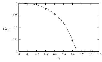
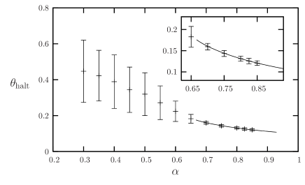
Figure 5: Left panel: probability of success of BP guided decimation on 3-xorsat random formulas, the solid line is the analytical prediction FrSu ; DeMo in the infinite size limit (cf. Eq.(39)), which vanishes for $\alpha>\alpha_{*}$, the symbols are the results of numerical simulations on 800 formulas of size $N=2\cdot 10^{4}$ variables for each value of $\alpha$. Right panel: the solid line is the curve $\theta_{+}(\alpha)$, symbols indicate the mean and variance (over unsuccesful runs) of the fraction of variables assigned before a contradiction is detected, from numerical simulations on 800 formulas of size $N=2\cdot 10^{4}$ variables for each value of $\alpha$.

In the left panel of Fig. 5 we present the probability of successful runs, with respect to the choice of the formula and to the randomness in the course of the run (order of the variables and free choices for unbiased marginals). It goes to a finite value in the thermodynamic limit (which can be computed analytically, see below) for $\alpha<\alpha_{*}$, and to 0 for $\alpha>\alpha_{*}$. A further piece of information is given in the right part of Fig. 5 about the number of steps performed by the algorithm (i.e. the number of variables assigned) before it stops. Let us call this random variable $T_{\rm halt}$ and the associated fraction $\theta_{\rm halt}=T_{\rm halt}/N$. We plotted the mean and variance (represented by error bars) of $\theta_{\rm halt}$, computed only on unsuccesful runs. For $\alpha<\alpha_{*}$ one finds that $\theta_{\rm halt}$ converges in the thermodynamic limit to a non trivial random variable. On the contrary in the regime where the algorithm fails w.h.p. (i.e. for $\alpha>\alpha_{*}$) the variance of $\theta_{\rm halt}$ vanishes at large $N$ (this result was obtained by performing the simulations at various sizes, which is not shown on the plot). In this case $\theta_{\rm halt}$ concentrates around its mean, which is found to coincide with the function $\theta_{+}(\alpha)$ defined above (see in particular the inset of the right panel of Fig. 5).

These numerical observations can now be interpreted in the light of the analytical computations performed above, which were mimicking the decimation process using the perfect marginals instead of the BP estimation. The threshold $\alpha_{*}$ above which the BP guided decimation algorithm fails w.h.p. coincides with the point where the evolution in the $(\alpha,\theta)$ phase diagram has to cross the transition lines drawn on Fig. 3, and in particular to penetrate the region $[\theta_{\rm c}(\alpha),\theta_{+}(\alpha)]$ where the 2-core of the residual formula only admits a sub-exponential number of solutions when the perfect marginals are used for the decimation. In this case the algorithm is naturally very sensitive to the small mistakes made by the BP algorithm, which destroy the few solutions of the 2-core. The fact that the residual formula is no longer satisfiable remains however unnoticed until a fraction $\theta_{+}(\alpha)$ of the variables have been assigned. At this point the fraction $\phi(\theta)$ of decimated and logically implied variables has a finite discontinuity (see right panel of Fig. 2), which means that the assignment of a few new variables triggers an avalanche of implications of extensive size. The extensive subgraph of newly implied variables will contain implication cycles which, if some mistakes have been done in the previous assignment steps, will lead to contradictions. More quantitatively, it was underlined above that $\theta_{+}(\alpha)$ marked the percolation of the subformula of length 2 clauses which supports the propagation of the logical implications.

The simplifying symmetries of the xor-satisfiability formulas are such that BP guided decimation is here almost equivalent to the Unit Clause Propagation algorithm with random heuristic (and also to the random pivoting Gaussian elimination algorithm of global ). The only slight difference between the two lies in the order in which the variables are treated, the logical implications being propagated as soon as they are detected in UCP. In the BP description of the algorithm the implication is effectively taken into account by the propagation of the messages, even if the variable is not explicitely declared as assigned. The behavior of UCP on xor-satisfiability formulas has been studied in xor3 , the results we just found are in agreement with the ones of this paper. In particular the phase diagram in Fig. 3 reproduces the left panel of Fig. 3 in xor3 , apart from the difference in the definition of the vertical time axis explained above. The equivalence with UCP allows also the computation of the probability of success in the thermodynamic limit for $\alpha<\alpha_{*}$. A detailed derivation for satisfiability formulas can be found in FrSu ; DeMo , we state here the result without proof,

$$P_{\rm succ}=\exp\left[-\int_{0}^{1}\frac{{\rm d}t}{4(1-t)}\frac{f(t)^{2}}{1-f(t)}\right]\qquad\text{with}\quad f(t)=\alpha k(k-1)t^{k-2}(1-t)\ .$$ (38)

For $k=3$ this expression can be further simplified,

$$P_{\rm succ}=\exp\left[\frac{3\alpha}{4}-\frac{1}{2}\frac{1}{\sqrt{\frac{\alpha_{*}}{\alpha}-1}}\arctan\left(\frac{1}{\sqrt{\frac{\alpha_{*}}{\alpha}-1}}\right)\right]\ .$$ (39)

This function is plotted as a solid line in the left panel of Fig. 5 and agrees with the results of the numerical experiments.

V Application to the SAT ensemble

We turn in this section to the case of random satisfiability formulas. We shall first apply the analytical cavity formalism to this particular model, then present the results of numerical experiments with the BP guided decimation algorithm and confront the two approaches.

V.1 BP equations

Let us begin by expliciting the BP equations (8) for the satisfiability constraints defined in (2). As the variables $\sigma_{i}$ are binary the messages $\{\nu_{a\to i}(\sigma_{i}),\eta_{i\to a}(\sigma_{i})\}$ can be parametrized with a single real for each, that we shall denote $\{u_{a\to i},h_{i\to a}\}$, under the form:

$$\nu_{a\to i}(\sigma_{i})=\frac{1-J_{i}^{a}\sigma_{i}\tanh u_{a\to i}}{2}\ ,\qquad\eta_{i\to a}(\sigma_{i})=\frac{1-J_{i}^{a}\sigma_{i}\tanh h_{i\to a}}{2}\ .$$ (40)

As we included the coupling contant $J_{i}^{a}$ in these definitions a positive value of, for instance $h_{i\to a}$, does not indicate a bias of $\sigma_{i}$ towards the value $+1$ in the absence of clause $a$, but rather towards the value $-J_{i}^{a}$ that does satisfy $a$. The message sent by a clause to one of its variables is then found to be

$$u_{a\to i}=f(\{h_{j\to a}\}_{j\in\partial a\setminus i})\ ,\qquad f(h_{1},\dots,h_{k-1})=-\frac{1}{2}\ln\left(1-\prod_{i=1}^{k-1}\frac{1-\tanh h_{i}}{2}\right)\ .$$ (41)

To give the explicit form of the other set of BP equations it is advisable to introduce some further definitions. We shall call $\partial_{+}i$ (resp. $\partial_{-}i$) the set of clauses in $\partial i$ which are satisfied by $\sigma_{i}=+1$ (resp. $\sigma_{i}=-1$), that is $\partial_{\sigma}i=\{a\in\partial i|J_{i}^{a}=-\sigma\}$. Moreover we let $\partial_{+}i(a)$ (resp. $\partial_{-}i(a)$) denote the set of clauses in $\partial i\setminus a$ agreeing (resp. disagreeing) with $a$ on the value $i$ should take. In formulae, $\partial_{+}i(a)=\{b\in\partial i\setminus a|J_{i}^{b}=J_{i}^{a}\}$, $\partial_{-}i(a)=\{b\in\partial i|J_{i}^{b}=-J_{i}^{a}\}$. With these notations the message sent by a variable to a clause reads

$$h_{i\to a}=\sum_{b\in\partial_{+}i(a)}u_{b\to i}-\sum_{b\in\partial_{-}i(a)}u_{b\to i}\ ,$$ (42)

while the marginal probability of a variable $i$ reads from (9):

$$\mu_{i}(\sigma_{i})=\frac{1+\sigma_{i}\tanh(H_{i})}{2}\ ,\qquad H_{i}=\sum_{a\in\partial_{+}i}u_{a\to i}-\sum_{a\in\partial_{-}i}u_{a\to i}\ .$$ (43)

Finally when a subset of variables $D$ is fixed to a reference configuration $\underline{\tau}_{D}$, the BP equations (41,42) are complemented with the boundary condition $h_{i\to a}^{\underline{\tau}_{D}}=-J_{i}^{a}\tau_{i}\infty$ when $i\in D$. Note that in all the numerical implementations of these equations we keep the hyperbolic tangent of the messages $u$ and $h$ which are free from this apparent singularity in the definition of $h$ around a decimated variable.

V.2 The usual cavity method

The replica symmetric version of the cavity method for non-decimated random satisfiability formulas, following the general formalism recalled in Sec. III.1, corresponds to a probabilistic interpretation of the BP equations (41,42) applied to random factor graphs. As the cardinality of $\partial i\setminus a$ converges to a Poisson random variable of parameter $\alpha k$ and the sign $J_{i}^{a}$ in the constraints definition are $\pm 1$ with probability one half, it follows that $|\partial_{+}i(a)|$ and $|\partial_{-}i(a)|$ converge to two independent Poisson random variables with parameter $\alpha k/2$, denoted $l_{+}$ and $l_{-}$ below. One has thus to look for the solution of the distributional equations corresponding to (41,42) for the random variables $h$ and $u$:

$$h\overset{\rm d}{=}\sum_{i=1}^{l_{+}}u_{i}-\sum_{i=1}^{l_{-}}v_{i}\ ,\qquad u\overset{\rm d}{=}f(h_{1},\dots,h_{k-1})\ .$$ (44)

In these equations $h_{1},\dots,h_{k-1}$ are independent copies of $h$, $u_{1},\dots,u_{l_{+}}$ and $v_{1},\dots,v_{l_{-}}$ are independent copies of $u$.

A numerical determination of the fixed point distributions solutions of these equations can be achieved by the population dynamics method, revivified in this context by MePa . This consists in representing the random variable $u$ (resp. $h$) by a sample of ${\cal N}$ elements $u_{1},\dots,u_{\cal N}$ (resp. $h_{1},\dots,h_{\cal N}$). The sample representing $h$ is initialized arbitrarily, for instance $h_{j}=0$ for all $j\in[1,{\cal N}]$, then the two samples are updated alternatively as follows. A new sample representing $u$ is obtained from the representation of $h$ by, independently for each $j\in[1,{\cal N}]$:

• drawing $k-1$ indices $i_{1},\dots,i_{k-1}$ independently, uniformly in $[1,{\cal N}]$

• setting $u_{j}=f(h_{i_{1}},\dots,h_{i_{k-1}})$

Subsequently the sample of $h$ is updated, for each $j$, by:

• drawing $l_{+}$ and $l_{-}$, two Poisson random variables of mean $\alpha k/2$

• drawing $l_{+}+l_{-}$ indices $i^{+}_{1},\dots,i^{+}_{l_{+}},i^{-}_{1},\dots,i^{-}_{l_{-}}$ independently, uniformly in $[1,{\cal N}]$

• setting $h_{j}=\sum_{n=1}^{l_{+}}u_{i^{+}_{n}}-\sum_{n=1}^{l_{-}}u_{i^{-}_{n}}$

The replica symmetric description of the solution space of random satisfiability formulas (first obtained with replica computations in ksat_RS ) is only valid for low enough values of $\alpha$. The 1RSB analysis at $m=1$, described in generic terms in Sec. III.1, has been performed on the satisfiability ensemble in pnas ; sat_long . For $k\geq 4$ one finds a clustering transition at $\alpha_{\rm d}$ and a condensation one at $\alpha_{\rm c}$, before the satisfiability transition $\alpha_{\rm s}$ determined in MeZe ; MePaZe ; MeMeZe (for instance $\alpha_{\rm d}\approx 9.38$, $\alpha_{\rm c}\approx 9.55$ and $\alpha_{\rm s}\approx 9.93$ for $k=4$). In the intermediate regime $[\alpha_{\rm d},\alpha_{\rm c}]$ the complexity of the relevant clusters is positive and vanishes at $\alpha_{\rm c}$, a point beyond which most of the solutions are contained in a sub-exponential number of clusters. The value $k=3$ happens to be a particular case, for which the intermediate regime with a positive complexity is absent, that we shall not consider in the following.

V.3 The computation of $\omega(\theta)$

Let us now apply the formalism of Sec. III.2 to ensemble of decimated random satisfiability formulas. Using the parametrization (40) of the messages the random variables $(\eta,\widetilde{\eta}^{\,\tau})_{\ell}$, $(\eta,\eta^{\tau})_{\ell}$ and $(\nu,\nu^{\tau})_{\ell}$ becomes random pairs of reals, respectively $(h,\widetilde{h}^{\tau})_{\ell}$, $(h,h^{\tau})_{\ell}$ and $(u,u^{\tau})_{\ell}$ for $\tau=\pm 1$. In the same spirit as we include the coupling constants in the definitions (40) of the fields $u$ and $h$, we also “gauge” the definition of these random variables such that $u^{+}$ (resp. $u^{-}$) corresponds to the message $u_{a\to i}^{\underline{\tau}_{D}}$ where $\underline{\tau}_{D}$ is drawn conditional on $\tau_{i}$ satisfying (resp. not satisfying) clause $a$. The recursion equations (18,19,20) then reads

$$(h,\widetilde{h}^{\tau})_{\ell}\overset{\rm d}{=}\begin{cases}(h,h^{\tau})_{\ell}&\text{with probability}\ 1-\theta\\ (h,\tau\infty)&\text{otherwise}\end{cases}\ ,\quad(h,h^{\tau})_{\ell}\overset{\rm d}{=}\left(\sum_{i=1}^{l_{+}}u_{i}-\sum_{i=1}^{l_{-}}v_{i},\sum_{i=1}^{l_{+}}u^{\tau}_{i}-\sum_{i=1}^{l_{-}}v^{-\tau}_{i}\right)\ ,$$ (45)

where $l_{\pm}$ are two independent Poisson random variables of parameter $\alpha k/2$ and the $(u_{i},u_{i}^{\tau})$ and $(v,v_{i}^{\tau})$ are independent copies of $(u,u^{\tau})_{\ell}$. Finally Eq. (20) translates into

$$(u,u^{\tau})_{\ell+1}\overset{\rm d}{=}\left(f(h_{1},\dots,h_{k-1}),f(\widetilde{h}^{\tau_{1}}_{1},\dots,\widetilde{h}^{\tau_{k-1}}_{k-1})\right)\ ,$$ (46)

where the configuration of the variables $\tau_{1},\dots,\tau_{k-1}$ is drawn with one of the two following probability laws according to the value of $\tau$,

$$\text{Prob}[\tau_{1},\dots,\tau_{k-1}|\tau=+,h_{1},\dots,h_{k-1}]=\prod_{i=1}^{k-1}\frac{1+\tau_{i}\tanh h_{i}}{2}\ ,$$ (47)

or

$$\text{Prob}[\tau_{1},\dots,\tau_{k-1}|\tau=-,h_{1},\dots,h_{k-1}]=\frac{1-\mathbb{I}(\tau_{1}=\dots=\tau_{k-1}=-1)}{1-\prod_{i=1}^{k-1}\frac{1-\tanh h_{i}}{2}}\prod_{i=1}^{k-1}\frac{1+\tau_{i}\tanh h_{i}}{2}\ .$$ (48)

The fields $h_{i}$ are the same for the computation of $u$ in (46) and in the probability law of the $\tau_{i}$’s expressed in (47,48). The two initial conditions correspond to $(h,h^{\tau})_{\ell=0}\overset{\rm d}{=}(h,h)$ for the initialization called $I_{0}$, and $(h,h^{\tau})_{\ell=0}\overset{\rm d}{=}(h,\tau\infty)$ for $I_{1}$. Finally the average entropy of the decimated random formulas reads from (22)

$$\omega= - \alpha k(1-\theta)\,\mathbb{E}\left[\sum_{\tau}\frac{1+\tau\tanh(u+h)}{2}\ln\left(\frac{1+\tanh u^{\tau}\tanh h^{\tau}}{2}\right)\right]$$ (49)

$$+ \alpha\,\mathbb{E}\left[\sum_{\tau_{1},\dots,\tau_{k}}\frac{1-\mathbb{I}(\tau_{1}=\dots=\tau_{k}=-1)}{1-\prod_{i=1}^{k}\frac{1-\tanh h_{i}}{2}}\prod_{i=1}^{k}\frac{1+\tau_{i}\tanh h_{i}}{2}\ln\left(1-\prod_{i=1}^{k}\frac{1-\tanh\widetilde{h}^{\tau_{i}}_{i}}{2}\right)\right]$$

$$+ (1-\theta)\,\mathbb{E}\left[\sum_{\tau}\frac{1+\tau\tanh\left(\sum_{i=1}^{l_{+}}u_{i}-\sum_{i=1}^{l_{-}}v_{i}\right)}{2}\ln\left(\sum_{\sigma}\prod_{i=1}^{l_{+}}\frac{1+\sigma\tanh u^{\tau}_{i}}{2}\prod_{i=1}^{l_{-}}\frac{1-\sigma\tanh v^{-\tau}_{i}}{2}\right)\right]\ .$$

A numerical determination of the distribution of the random variables $(h,h^{\tau})_{\ell}$ and $(u,u^{\tau})_{\ell}$ can be performed by a population dynamics algorithm. We introduce two population of ${\cal N}$ triplets of reals, $\{(h_{i},h_{i}^{+},h_{i}^{-})\}_{i=1}^{\cal N}$ and $\{(u_{i},u_{i}^{+},u_{i}^{-})\}_{i=1}^{\cal N}$, such that, for instance, the empirical distribution of $(h_{i},h_{i}^{+})$ after $\ell$ steps of the algorithm is a good approximation of the random variable $(h,h^{+})_{\ell}$. In the initialization step of the algorithm the $h_{i}$’s are drawn according to the fixed point solution of Eq. (44), which is obtained from a preliminary RS population dynamics procedure. For the initial condition $I_{0}$ (resp. $I_{1}$) one sets $h_{i}^{+}=h^{-}_{i}=h_{i}$ (resp. $h_{i}^{\pm}=\pm\infty$) for all $i\in[1,{\cal N}]$. Then the following two kind of updates are iterated $\ell$ times. A new sample of $\{(u_{i},u_{i}^{+},u_{i}^{-})\}_{i=1}^{\cal N}$ is obtained by, independently for each $j\in[1,{\cal N}]$:

• drawing $k-1$ indices $i_{1},\dots,i_{k-1}$ independently, uniformly in $[1,{\cal N}]$

• setting $u_{j}=f(h_{i_{1}},\dots,h_{i_{k-1}})$

• independently for $n=1,\dots,k-1$

  • with probability $\theta$ set $\widetilde{h}^{+}_{n}=+\infty$ and $\widetilde{h}^{-}_{n}=-\infty$

  • otherwise set $\widetilde{h}^{+}_{n}=h_{i_{n}}^{+}$, and $\widetilde{h}^{-}_{n}=h_{i_{n}}^{-}$

• generating a configuration $\tau_{1},\dots,\tau_{k-1}$ from the law $\text{Prob}[\tau_{1},\dots,\tau_{k-1}|\tau=+,h_{i_{1}},\dots,h_{i_{k-1}}]$ defined in Eq.(47)

• setting $u^{+}_{j}=f(\widetilde{h}^{\tau_{1}}_{1},\dots,\widetilde{h}^{\tau_{k-1}}_{k-1})$

• generating a configuration $\tau_{1},\dots,\tau_{k-1}$ from the law $\text{Prob}[\tau_{1},\dots,\tau_{k-1}|\tau=-,h_{i_{1}},\dots,h_{i_{k-1}}]$ defined in Eq.(48)

• setting $u^{-}_{j}=f(\widetilde{h}^{\tau_{1}}_{1},\dots,\widetilde{h}^{\tau_{k-1}}_{k-1})$

Subsequently the sample of $\{(h_{i},h_{i}^{+},h_{i}^{-})\}_{i=1}^{\cal N}$ is updated, for each $j$, by:

• drawing $l_{+}$ and $l_{-}$, two Poisson random variables of mean $\alpha k/2$

• drawing $l_{+}+l_{-}$ indices $i^{+}_{1},\dots,i^{+}_{l_{+}},i^{-}_{1},\dots,i^{-}_{l_{-}}$ independently, uniformly in $[1,{\cal N}]$

• setting $h_{j}=\sum_{n=1}^{l_{+}}u_{i^{+}_{n}}-\sum_{n=1}^{l_{-}}u_{i^{-}_{n}}$, $h_{j}^{+}=\sum_{n=1}^{l_{+}}u^{+}_{i^{+}_{n}}-\sum_{n=1}^{l_{-}}u^{-}_{i^{-}_{n}}$ and $h_{j}^{-}=\sum_{n=1}^{l_{+}}u^{-}_{i^{+}_{n}}-\sum_{n=1}^{l_{-}}u^{+}_{i^{-}_{n}}$

After a large number of these iterations has been performed the determination of the residual entropy (49) is easily obtained: the expectation values can be interpreted as empirical averages over the population.

We have implemented this numerical procedure and performed the computation for various values of $\alpha$ and $\theta$. The results for $k=4$ are as follows. For small enough values of $\alpha$ the large $\ell$ limit of the recursion relations (45,46) is found to be independent of the initial condition $I_{0}$ or $I_{1}$ used, and the residual entropy density $\omega(\theta)$ is a smoothly decreasing function. This quantity is plotted for $\alpha=8.8$ on the left panel of Fig. 6. For larger values of $\alpha$ there appears a regime $\theta\in[\theta_{-}(\alpha),\theta_{+}(\alpha)]$ in which the two initial conditions leads to different fixed point solutions of (45,46), signaling the presence of non-trivial long range point-to-set correlations in the decimated formula. The two branches of $\omega(\theta)$ are plotted in the right panel of Fig. 6 for $\alpha=9.3$, and are found to cross each other at $\theta_{\rm c}(\alpha)\in[\theta_{-}(\alpha),\theta_{+}(\alpha)]$. For $\theta\in[\theta_{-}(\alpha),\theta_{\rm c}(\alpha)]$ the branch with the highest value of $\omega$ corresponds to the $I_{0}$ initialization, the situation being reversed for $\theta\in[\theta_{\rm c}(\alpha),\theta_{+}(\alpha)]$. As explained on the simpler xorsat example, we interpret these results as following from the existence of a positive complexity of relevant clusters in the regime $[\theta_{-},\theta_{\rm c}]$. In this case the highest branch of $\omega(\theta)$ is the total entropy of the decimated formula, while the difference between the two branches is its complexity. On the contrary for $[\theta_{\rm c},\theta_{+}]$ the upper branch is the only relevant one, the total entropy is dominated by the subexponential number of clusters around a typical reference solution $\underline{\tau}$. The three critical lines are displayed in the $(\alpha,\theta)$ of Fig. 7, which also shows that, as follows from their definitions, $\theta_{-}(\alpha)$ (resp. $\theta_{\rm c}(\alpha)$) reaches the horizontal axis $\theta=0$ at the usual dynamic transition $\alpha_{\rm d}$ (resp. condensation threshold $\alpha_{\rm c}$). We estimated the location of the critical point where $\theta_{\pm}$ and $\theta_{\rm c}$ merge to be $\alpha_{*}=9.05$, $\theta_{*}=0.045$, by interpolation of the results obtained for values of $\alpha$ slightly larger.

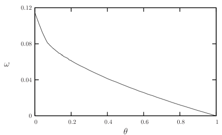
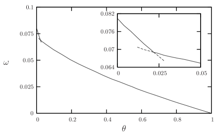
Figure 6: Residual entropy $\omega(\theta)$ of 4-sat random formulas. Left panel: $\alpha=8.8$, $\omega(\theta)$ is smoothly decreasing. Right panel: $\alpha=9.3$, the inset is a zoom around the singular point of $\omega(\theta)$.

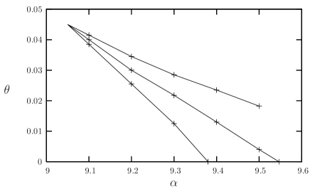
Figure 7: Phase diagram of 4-sat random formulas in the $(\alpha,\theta)$ plane, from bottom to top $\theta_{-}(\alpha)$, $\theta_{\rm c}(\alpha)$ and $\theta_{+}(\alpha)$. Symbols result from the population dynamics algorithm, lines are guides to the eye.

V.4 The computation of $\phi(\theta)$

We proceed now with the computation of the fraction of logically implied variables, following the lines sketched in Sec. III.3 (the same results were presented in allerton with a slightly different formulation).

Let us first discuss the Warning Propagation equations for satisfiability formulas. According to the projection equations (11) one has to identify the situations in which a single value of a variable $\sigma_{i}$ is allowed by a BP message. For the messages sent by a clause to a variable this can only happen when the variable is forced to satisfy the clause, i.e. $\nu_{a\to i}(\sigma_{i})=\delta_{\sigma_{i},-J_{i}^{a}}$, in which case we define the WP message to be ${\mathfrak{u}}_{a\to i}=1$, otherwise ${\mathfrak{u}}_{a\to i}=0$. A message $\eta_{i\to a}$ sent from a variable to a clause can allow both values of variable $\sigma_{i}$, or force it to the value satisfying $a$ ($\eta_{i\to a}(\sigma_{i})=\delta_{\sigma_{i},-J_{i}^{a}}$), or to the value disastifying it ($\eta_{i\to a}(\sigma_{i})=\delta_{\sigma_{i},J_{i}^{a}}$). It is only the latter case that shall be propagated by the WP equations, we thus affect the value ${\mathfrak{h}}_{i\to a}=0$ to the first two situations and ${\mathfrak{h}}_{i\to a}=1$ to the latter. The WP equations read with these definitions:

$${\mathfrak{u}}_{a\to i}=\prod_{j\in\partial a\setminus i}{\mathfrak{h}}_{j\to a}\ ,\qquad{\mathfrak{h}}_{i\to a}=1-\prod_{b\in\partial_{-}i(a)}(1-{\mathfrak{u}}_{b\to i})\ .$$ (50)

For a variable $i\in D$ the boundary condition reads ${\mathfrak{h}}_{i\to a}=\mathbb{I}(\tau_{i}=J_{i}^{a})$.

In order to compute the average fraction of logically implied variables, within the assumptions of the RS cavity method on the local description of the uniform probability measure $\mu(\cdot)$, we introduce the sequences of random variables $(h,\widetilde{{\mathfrak{h}}}^{\tau})_{\ell}$, $(h,{\mathfrak{h}}^{\tau})_{\ell}$ and $(u,{\mathfrak{u}}^{\tau})_{\ell}$ as defined in Sec. III.3. It turns out that not all the values of $\tau$ have to be considered. Consider for instance the random variable $(u,{\mathfrak{u}}^{\tau})_{\ell}$. Its distribution is by definition the one of $(u_{a\to i},{\mathfrak{u}}_{a\to i}^{\underline{\tau}_{D}})$, in the random tree model of depth $\ell$, rooted at variable $i$ which appears solely in the clause $a$. Depending on $\tau$ the reference configuration $\underline{\tau}$ is drawn conditional on $\tau_{i}$ either satisfying (if $\tau=+1$) or not satisfying ($\tau=-1$) the constraint $a$. In the latter case ${\mathfrak{u}}_{a\to i}^{\underline{\tau}_{D}}$ is necessarily equal to 0: at least one of the variables in $\partial a\setminus i$ must satisfy $a$ in $\underline{\tau}$, and this variable cannot be forced to its opposite value by $\underline{\tau}_{D}$. We can hence restrict our attention to $(u,{\mathfrak{u}}^{+})_{\ell}$, which is found to obey

$$(u,{\mathfrak{u}}^{+})_{\ell+1}\overset{\rm d}{=}(f(h_{1},\dots,h_{k-1}),\zeta\,\widetilde{{\mathfrak{h}}}_{1}^{-}\dots\widetilde{{\mathfrak{h}}}_{k-1}^{-})\ ,\qquad\zeta\overset{\rm d}{=}\begin{cases}1&\text{with probability}\ \prod_{i=1}^{k-1}\frac{1-\tanh h_{i}}{2}\\ 0&\text{otherwise}\end{cases}\ .$$ (51)

The probability that the random variable $\zeta$ equals $1$ is indeed the probability that, conditional on $\tau_{i}$ satisfying the root clause $a$, the configuration of the $k-1$ other variables in $\partial a\setminus i$ are drawn to the values unsatisfying $a$.

For similar reasons the right hand side of this equation does not depend on $(h,\widetilde{{\mathfrak{h}}}^{+})$ and we can complete this equation with the recursion on $(h,\widetilde{{\mathfrak{h}}}^{-})$ and $(h,{\mathfrak{h}}^{-})$, which read

$$(h,\widetilde{{\mathfrak{h}}}^{-})_{\ell}\overset{\rm d}{=}\begin{cases}(h,{\mathfrak{h}}^{-})_{\ell}&\text{with probability}\ 1-\theta\\ (h,1)&\text{otherwise}\end{cases}\ ,\quad(h,{\mathfrak{h}}^{-})_{\ell}\overset{\rm d}{=}\left(\sum_{i=1}^{l_{+}}u_{i}-\sum_{i=1}^{l_{-}}v_{i},1-\prod_{i=1}^{l_{-}}(1-{\mathfrak{v}}_{i}^{+})\right)\ ,$$ (52)

where as usual $l_{\pm}$ are two Poisson random variables of parameter $\alpha k/2$ and the $(u_{i},{\mathfrak{u}}_{i}^{+})$ and $(v_{i},{\mathfrak{v}}_{i}^{+})$ are independent copies of $(u,{\mathfrak{u}}^{+})_{\ell}$. Finally the average fraction of either decimated or directly implied variables can be obtained as

$$\phi(\theta)=\mathbb{E}[(1-\tanh h)\widetilde{{\mathfrak{h}}}^{-}]\ .$$ (53)

These recursion equations can be solved numerically using the same kind of population dynamics as explained above, updating in turns populations of pairs $\{(h_{i},{\mathfrak{h}}_{i}^{-})\}_{i=1}^{\cal N}$ and $\{(u_{i},{\mathfrak{u}}_{i}^{-})\}_{i=1}^{\cal N}$. The two kind of initial conditions already discussed correspond here to $(h,{\mathfrak{h}}^{-})_{\ell=0}\overset{\rm d}{=}(h,0)$ for $I_{0}$, and $(h,{\mathfrak{h}}^{-})_{\ell=0}\overset{\rm d}{=}(h,1)$ for $I_{1}$.

This numerical resolution leads to the following results for $k=4$. At small enough values of $\alpha$ the two initial conditions lead to the same large $\ell$ limit, the function $\phi(\theta)$ is smoothly increasing (see left panel of Fig. 8). For larger values of $\alpha$ there exists a range of parameter $[\theta^{\prime}_{-}(\alpha),\theta^{\prime}_{+}(\alpha)]$ where the quantity (53), computed from the initial condition $I_{1}$, is strictly greater than the one reached from $I_{0}$. In this coexistence regime we shall call $\psi(\theta)$, in analogy with the notations used for the xorsat model, the upper branch obtained from $I_{1}$, see for instance the right panel of Fig. 8. The function $\phi$ (resp. $\psi$) is discontinuous at $\theta^{\prime}_{+}$ (resp. $\theta^{\prime}_{-}$). These two thresholds are the two upper curves in the phase diagram of Fig. 9, which also contains for comparison a repetition of the phase diagram of Fig. 7. The two regimes for the behaviour of $\phi(\theta)$ are separated by the value $\alpha^{\prime}_{*}\approx 8.05$.

At this point the reader might be puzzled by the apparent contradiction between these results and those of the previous subsection. Consider indeed some parameters $\alpha>\alpha^{\prime}_{*}$ and $\theta\in[\theta^{\prime}_{-}(\alpha),\theta^{\prime}_{+}(\alpha)]$. We claimed in the previous subsection that the large $\ell$ limit of the random variable $(h,h^{\tau})_{\ell}$ was independent of the initial condition in $\ell=0$, whereas we just found that $(h,{\mathfrak{h}}^{-})_{\ell}$ does depend on it. As the latter variable is a projection of the former, this statement is at first sight paradoxical. This apparent contradiction can however be resolved by a closer inspection of the relationship between the two random variables. One has indeed

$$(h,{\mathfrak{h}}^{-})_{\ell}\overset{\rm d}{=}\lim_{\varepsilon\to 0}(h,\mathbb{I}(\tanh h^{-}\leq-1+\varepsilon))_{\ell}\ ,$$ (54)

while the two apparently contradictory statements are

$$\lim_{\ell\to\infty}(h,h^{-})_{\ell}^{I_{0}}\overset{\rm d}{=}\lim_{\ell\to\infty}(h,h^{-})_{\ell}^{I_{1}}\ ,\qquad\lim_{\ell\to\infty}(h,{\mathfrak{h}}^{-})_{\ell}^{I_{0}}\overset{\rm d}{\neq}\lim_{\ell\to\infty}(h,{\mathfrak{h}}^{-})_{\ell}^{I_{1}}\ .\qquad$$ (55)

The resolution of the paradox relies on the non-commutativity of the limits $\ell\to\infty$ and $\varepsilon\to 0$. More explicitly, under the initialization $I_{0}$ there is a positive probability for a field $\tanh h^{-}$ to have -1 as its large $\ell$ limit, yet remaining strictly superior to -1 as long as $\ell$ is finite. If the limit $\varepsilon\to 0$ is taken before $\ell\to\infty$ these fields do not participate to ${\mathfrak{h}}^{-}$, which is thus found to be smaller in the initialization $I_{0}$ with respect to $I_{1}$. Yet if the limit $\ell\to\infty$ is performed first this positive fraction of the fields $\tanh h^{-}$ (with initialization $I_{0}$) reach their limit $-1$, hence making possible the first statement of Eq. (55). We checked explictly this phenomenon by constructing a coupling of the two initializations and solved it with the population dynamics algorithm.

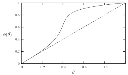
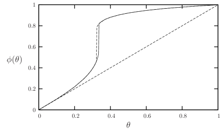
Figure 8: Fraction $\phi(\theta)$ of assigned and logically implied variables in 4-sat random formulas , left: $\alpha=7.0$, right: $\alpha=8.4$.

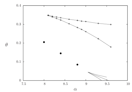
Figure 9: Phase diagram of 4-sat random formulas in the $(\alpha,\theta)$ plane. The three lines in the bottom of the figure are those of Fig. 7, the upper two are $\theta^{\prime}_{-}(\alpha)<\theta^{\prime}_{+}(\alpha)$ defined in Sec. V.4 from the discontinuities of $\phi(\theta)$ and $\psi(\theta)$. The filled circles show the location $\theta_{\rm max}(\alpha)$ of the slowest convergence of the BP iterations in the BP guided decimation algorithm, see Sec. V.5.2.

V.5 Numerical experiments on BP guided decimation

We have run the belief propagation guided decimation algorithm for many random 4-sat formulas. The sizes of the formulas studied are $N=10^{3},3\times 10^{3},10^{4},3\times 10^{4}$, with $\alpha$ varying between $6.0$ and $9.2$. The number of formulas analyzed varies with $\alpha$, but it is always larger than 2000 for $N=10^{3}$, larger than 1200 for $N=3\times 10^{3}$, larger than 400 for $N=10^{4}$ and between 360 and 25 (increasing $\alpha$) for $N=3\times 10^{4}$.

V.5.1 Details on the practical implementation

Some technical details about the numerical implementation of the BP guided decimation algorithm were given in allerton (see also Appendix A of sat_long for details on the representation of BP messages and probabilities). The main numerical bottleneck in applying the BP guided decimation algorithm is the convergence of the iterative method for solving the BP equations, described in Section II.4. This iterative scheme is known to be a fast way of finding a fixed point of the BP equations, although sometimes it may not converge. Lack of convergence may be due to different reasons: in case long range correlations develop, multiple BP fixed points appear and the convergence of BP to one of these fixed point cannot be guaranteed; on the other hand, when a single BP fixed point exists, convergence problems can be typically cured by the use of a damping term Pretti . In all our numerical simulations we have used a damping term of intensity 0.1, that is, when we update a message x, we do not assign to it directly the new value xNew, but rather the weighted sum 0.9 * xNew + 0.1 * x. We have verified that under these conditions the convergence (if any) is always exponentially fast in the number of iterative steps (although sometimes with an exponent very small). Because of the exponentially fast convergence, our arbitrary choice of considering BP equations solved when the maximal change in any BP message is below $10^{-4}$ turns out to be very reasonable: indeed an accuracy of $10^{-8}$ can be reached by simply doubling the running time. Anyhow, in order to avoid entering a never-ending loop we have also fixed a maximum number of iterations equal to 1000; when this limit is reached non-converged BP messages are used to compute marginals and to proceed with the decimation.

The last comment about technical issues regards the initialization of BP messages before the iterative solving procedure is applied. At the beginning, when the formula is still not decimated, BP messages are initialized in a random way assigning to each $\tanh(h_{i\to a})$ a random value uniformly distributed between $-0.2$ and $0.2$. After each variable decimation, one can choose to keep the BP messages obtained from the last iterative procedure or to re-initialize them along the same random way described above. In principle, if a single BP fixed point exists and if this is reached by the iterative method, then the starting point should be irrelevant. Moreover, one would expect that the BP fixed points of two formulas differing in just a variable are very close, and that starting from the one already reached should help convergence (with respect to start from random messages). This intuition turns out to be wrong. We have strong numerical evidence that a random re-initialization of BP messages after each decimation strongly enhances the performances of the algorithm. A possible explanation is the following. Our numerical procedure does not produce a perfect estimation of the marginal probabilities (in particular when the stopping criterion used is the maximal number of iterations); if messages are not re-initialized small errors may easily accumulate in the same direction, while a random re-initialization of BP messages results in a partial neutralization of these errors.

V.5.2 Algorithm performances and convergence probabilities

Figure 10: Success probability of the BP guided decimation algorithm as a function of $\alpha$ for random 4-sat formulas of various sizes. The vertical line marks the value $\alpha_{*}=9.05$ beyond which the analytical computations predicted a condensation transition in the residual entropy $\omega(\theta)$.

As a first result, we show in Fig. 10 the success probability for the BP guided decimation algorithm, i.e. the fraction of formulas which have been solved by this algorithm. The numerical data clearly point to an algorithmic threshold $\alpha_{\rm a}$ very close to the theoretical prediction of the point $\alpha_{*}=9.05$ (marked by a vertical line in Fig. 10) above which phase transitions occur in the thermodynamic properties of the decimated ensemble of random formulas. For $\alpha<\alpha_{\rm a}$ a large $N$ formula is solved with positive probability by the BP guided decimation algorithm. The appearance of a jump in the function $\phi(\theta)$ at $\alpha\simeq 8.1$ [see below for a more detailed analysis of $\phi(\theta)$], with a consequent avalanche of directly implied variables during the decimation of formulas with $\alpha>8.1$, does not have any visible effect on the success probability. This phenomenon has however a trace in the random variable $\theta_{\rm halt}$, that is the fraction of variables assigned before the discovery of a contradiction during the unsuccesful runs. The distribution of this random variable is shown in Fig. 11 for two values of $\alpha$ (below and above $\alpha_{\rm a}$). One can see a maximum in this distribution for values of $\theta$ slightly smaller than $\theta^{\prime}_{+}(\alpha)$, the point of discontinuity of $\phi(\theta)$.

Figure 11: Distribution of the halting time of the BP guided decimation algorithm on 4-sat random formulas with $\alpha=8.4$ (left panel) and $\alpha=9.2$ (right panel). Vertical lines show the value of $\theta^{\prime}_{+}(\alpha)$ where $\phi(\theta)$ is discontinuous.

Figure 12: Probability of non convergence in 1000 iterations (upper panels) and average number of iterations required to reach convergence (lower panels) for the BP part of the BP guided decimation algorithm, as a function of the fraction $\theta$ of decimated variables. From left to right $\alpha=7$, $\alpha=8$, $\alpha=8.4$, $\alpha=8.8$.

In the following we are going to present data only in the region $\alpha<\alpha_{\rm a}$. In order to reduce finite size effects we will concentrate only on formulas which have been actually solved by our algorithm. The study of the convergence probability and of the average convergence time for the iterative method used to solve the BP equations provides very useful information, as it allows to identify the most difficult formulas, which should appear close to the threshold. In Fig. 12 we show both the probability that the BP fixed point is not reached after 1000 iterations (upper panels) and the average number of iterations required to converge (lower panels). Non-converged instances count with 1000 in the average. Four values of $\alpha$ are shown (from left to right), $\alpha=7.0$, $8.0$, $8.4$ and $8.8$, and $\theta>0.5$ is not shown since in that region nothing of interest takes place.

We see that, for small values of $\alpha$, by increasing the size of formulas the probability that BP does not converge in 1000 steps reduces considerably, thus suggesting that in the large $N$ limit the typical running time of BP is below 1000 for any $\theta$ value. On the contrary, for larger values of $\alpha$, the probability that BP does not converge is not varying very much with $N$ and seems to remain positive even in the large $N$ limit, thus suggesting that the typical number of iterations required to make BP converge is larger than 1000 for some values of $\theta$.

The overall picture we get from Fig. 12 is very clear. For any $\alpha$ value, the decimation procedure initially produces formulas which are more and more difficult to solve and the running time of BP thus increases with $\theta$. The running time (or equivalently the probability of not converging in a fixed number of iterations) has a maximum at a value $\theta_{\rm max}(\alpha)$ and then decreases again. By increasing $\alpha$, $\theta_{\rm max}(\alpha)$ decreases and the running time at $\theta_{\rm max}$ increases. It is natural to expect that the maximum running time should diverge at the threshold $\alpha_{\rm a}$; moreover, if one assumes that this phenomenon is related to the critical point $\alpha_{*}$ marking the end of the (first-order) condensation transition line $\theta_{\rm c}(\alpha)$ for $\alpha>\alpha_{*}$, one should expect that $\theta_{\rm max}(\alpha)$ is a precursor of the transition line $\theta_{\rm c}(\alpha)$ in the phase $\alpha<\alpha_{*}$. The data of $\theta_{\rm max}(\alpha)$ plotted with filled circles in Fig. 9 are in agreement with this intuition, showing in particular that $\theta_{\rm max}(\alpha)$ reaches values very close to $\theta_{*}$ for the largest values of $\alpha$ the algorithm is able to handle.

V.5.3 Entropy of decimated formulas

We measured the entropy of decimated formulas along the execution of the BP guided decimation algorithm, using the Bethe approximation stated in (10). When comparing these results with the analytic prediction presented in Section V.3, a lot of care is required in dealing with cases where BP did not converge to a fixed point. Indeed in these cases the marginal probabilities do not satisfy the consistency constraints and the resulting value for the entropy may be quite far from the correct one. In order to avoid this problem we have adopted a drastic, but safe approach: we take the average over only those formulas for which the algorithm always converged before reaching the 1000 iterations limit. A possible criticism to this approach is that we are taking the average over the simplest formulas, thus obtaining a biased estimate for the residual entropy. If this criticism is well founded we should observe a dependence of the average residual entropy upon the value of maximal number of iterations. Actually we do not observe any variation by doubling the maximal number of iterations.

Figure 13: Residual entropy as a function of the fraction $\theta$ of decimated variables for $\alpha=7$ (upper curves) and $\alpha=8.4$ (lower curves). The symbols correspond to the analytical predictions presented in Sec. V.3, the lines to the numerical simulations of the BP guided decimation algorithm for various sizes.

In Fig. 13 we plot the residual entropy as a function of $\theta$ for three different sizes (lines) together with the analytical predictions of Sec. V.3 (points with errors). For $\alpha=7.0$, even the $N=10^{3}$ data are almost superimposed to the analytic result. On the contrary, for $\alpha=8.4$ finite size effects are much more evident and only $N=10^{4}$ data start to be compatible with the analytical computations in the thermodynamic limit.

It is also worth noticing that the function $\omega(\theta)$ shows its point of maximum curvature close to $\theta_{\rm max}$. More in general the curvature of $\omega(\theta)$ seems to be somehow related to the typical running time of BP.

V.5.4 Forced variables and multiple WP fixed points

Figure 14: The fraction $\phi(\theta)$ of assigned and logically implied variables for $4$-sat formulas of density $\alpha=7$ and $\alpha=8.4$. The insets detail the results at $\alpha=8.4$ for the decimation and backward algorithm, see the text for details.

We also keep track of the fraction of logically implied variables in the partially decimated formulas, measuring it with the WP algorithm (equivalent to UCP as explained in Sec. II.4). In the main panel of Fig. 14 we plot the function $\phi(\theta)$ computed analytically (solid curves). For $\alpha=7.0$ the function $\phi(\theta)$ is smoothly increasing and the numerical data follow this curve so nicely that only the $N=10^{3}$ data is hardly visible, the rest being perfectly superimposed to the analytic curve. For $\alpha=8.4$ the function $\phi(\theta)$ is multivalued in the interval $[\theta^{\prime}_{-}(\alpha),\theta^{\prime}_{+}(\alpha)]$ and the two curves plotted in the main panel correspond to the two branches $\phi(\theta)$ and $\psi(\theta)$ defined in Sec. V.4. The numerical data for $\alpha=8.4$ are shown in the insets for clarity. The left inset corresponds to the decimation algorithm (which indeed increases $\theta$ during the run). The right inset reports the data gathered while running the backward algorithm which works as follows.

After a succesful run of the BP guided decimation algorithm we use the solution $\underline{\tau}$ constructed as the reference one, and variables are unfixed one by one in the reverse fixing order: in this way at any $\theta$ value the residual formula is exactly the same the decimation algorithm had to work with. The only differences between the two algorithms are the initial values for the WP and BP messages: in the backward algorithm all messages are set initially according to the solution found in $\theta=1$, namely $\tanh h_{i\to a}=-J_{i}^{a}\tau_{i}$ and ${\mathfrak{h}}_{i\to a}=\mathbb{I}(\tau_{i}=J_{i}^{a})$ for all edges. Then the updates of WP and BP are run as usual for the edges outside the decimated ones. The numerical data shown in the insets suggest that, although finite size effects are huge, in the large $N$ limit the decimation (resp. the backward) algorithm follow the lower branch $\phi(\theta)$ (resp. upper branch $\psi(\theta)$) curve shown in the main panel. As predicted by the analytical computation, for $\alpha>\alpha^{\prime}_{*}\simeq 8.05$ the fraction of variables which are frozen (either assigned or directly implied by WP), $\phi(\theta)$, has a hysteresis loop when the number of assigned variables $\theta$ is increased and decreased across the interval $[\theta^{\prime}_{-}(\alpha),\theta^{\prime}_{+}(\alpha)]$, the backward algorithm used when decreasing $\theta$ corresponding to the $I_{1}$ boundary condition of the infinite tree computation. The hysteresis loop obtained by looking at the WP messages is reported with a full line in Fig. 15 (where data for $N=3\times 10^{4}$ and $\alpha=8.4$ are used).

Figure 15: Fraction of frozen variables as a function of $\theta$, for $\alpha=8.4$. The full lines correspond to the WP results in the decimation and backward algorithm, the dashed lines to the analysis of the BP messages.

The apparent paradox discussed at the end of Sec. V.4 shows up here again, at the level of the single sample analysis instead of the computation on the infinite tree: the forward and backward procedure allows us to construct two distinct fixed points of the WP equations on the same partially decimated formula (see points A and B in Fig. 15), while the success probability of the algorithm is still positive for this value of $\alpha$ and the residual entropy of Fig. 13 has no singularity. In addition to the above discussion on the non-commutativity between the projection from WP to BP and the limit of infinite depth tree/number of iterative updates, it is worth noting that with the initial condition used in the backward algorithm the Warning Propagation procedure corresponds actually to the whitening construction (see for instance Maneva ), starting from the solution found at the end of the forward algorithm. The interpretation of the number of frozen variables in A and B is thus different: A corresponds to the variables which are logically implied (in the UCP sense) in the partially decimated formula. On the other hand B counts the number of constrained variables in the core Maneva of the reference solution of the partially decimated formula (the one reached by the decimation). The existence of distinct WP fixed points would be a sign of a positive SP complexity if one assumed these fixed points to be exponentially numerous. Even when this assumption is correct it does however not lead to a contradiction with the inexistence of thermodynamically relevant clusters or long-range correlations as defined in (23). The former corresponds indeed to a 1RSB computation with Parisi parameter $m=0$ and the latter to $m=1$. We checked indeed that computing the residual entropy with the backward algorithm yields the same result as with the decimation one, whereas in presence of an extensive thermodynamical complexity we would have obtained only the contribution from the internal entropy of the cluster around the reference solution.

More indications come from the study of BP fixed point messages. In Fig. 15 we plot the fraction of variables that receive BP messages forcing it to a unique value (BP frozen) and the fraction of variables which are extremely biased under the BP messages, i.e. the less probable value has a probability smaller than $10^{-10}$ (BP prob$<10^{-10}$). The fraction of BP frozen variables again shows hysteresis: in the decimation algorithm BP frozen variables perfectly coincide with WP frozen variables, while in the backward algorithm BP frozen variables are a little more than WP frozen variables because of the numerical impossibility of keeping marginals arbitrarily small. What is more interesting is that the fraction of extremely biased variables (BP prob$<10^{-10}$) does not show any sign of hysteresis: the same smooth curve is followed by the decimation algorithm as well as by the backward algorithm. This observation suggests that BP marginals obtained by the two algorithms are exactly the same, except for (almost) completely frozen variables.

V.6 Large $k$ behaviour

We have seen that the behaviour of the ensemble of decimated random formulas is richer in the satisfiability case than for xor-satisfiability, with in particular the appearance of two sets of critical lines, one describing the thermodynamic properties, $\omega(\theta)$, and the other the singularities of the logical implications, $\phi(\theta)$. The common wisdom is however that when the length $k$ of the clauses gets large the satisfiability model gets simpler, notably allowing some tight rigorous results largek_1 ; largek_2 ; largek_3 ; largek_4 , and in fact becomes very similar to the xor-satisfiability one. We shall hence briefly discuss now the large $k$ limit of our results for the decimated ensembles.

Let us begin with the xor-satisfiability case; the results of Sec. IV having an explicit form, they can be easily turned in asymptotic expansions for large $k$. For instance the threshold $\alpha_{*}$ given in Eq. (33) is found to behave as $\frac{e}{k}(1+O(k^{-1}))$, while the clustering threshold $\alpha_{\rm d}$ is $\frac{\ln k}{k}(1+O(\ln\ln k/\ln k))$ and the condensation threshold $\alpha_{\rm c}$ goes to 1 in the large $k$ limit. One can also study the behaviour of the transition line $\theta_{\rm c}(\alpha)$ in the last of these three asymptotic scales (i.e. for $\alpha$ constant with respects to $k$). After a short computation, which consists in expanding the fixed point solutions $\phi(\theta)$ and $\psi(\theta)$ of Eq.(32), and the associated entropies (35), one finds that the two leading orders are $\theta_{\rm c}(\alpha)\sim 1-\alpha-\alpha e^{-\alpha k}$.

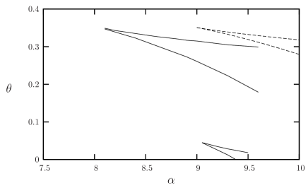
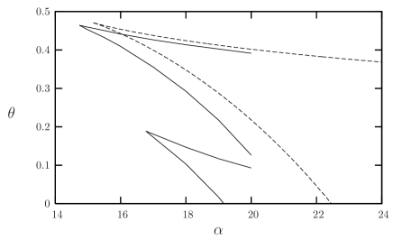
Figure 16: Critical lines $\theta_{\pm}(\alpha)$ and $\theta^{\prime}_{\pm}(\alpha)$ for $k$-satisfiability, left: $k=4$, right: $k=5$. The dashed lines are the $k$-xorsatisfiability critical lines, with a rescaling of $2^{k}$ on their clause density.

Large $k$ asymptotic expansions of the non-decimated ($\theta=0$) ensemble of $k$-satisfiability were performed for the clustering and condensation thresholds in sat_long and in MeMeZe for the satisfiability one. The leading order of the clustering threshold is $2^{k}\frac{\ln k}{k}$, while both condensation and satisfiability occurs for values of $\alpha$ around $2^{k}\ln 2$ (see sat_long ; MeMeZe for the subleading corrections, which are different for $\alpha_{\rm c}$ and $\alpha_{\rm s}$). Consider now the fraction of decimated or implied variables $\phi(\theta)$, computed for the satisfiability ensemble according to Eqs. (51,52). In the large $k$ limit a crucial simplification occurs thanks to the concentration, at the leading order, of the $h$ and $u$ random variables solutions of the RS equation (44) around 0. From this fact follows easily (compare with Eqs. (30,31)) that the functions $\phi(\theta)$ and $\psi(\theta)$, for satisfiability random formulas of clause density $\alpha$, approach the corresponding functions of xor-satisfiability formulas of clause density $\alpha/2^{k}$. In consequence this correspondence holds for the lines $\theta^{\prime}_{\pm}(\alpha)$, and the critical point $\alpha^{\prime}_{*}$ of satisfiability is expected to scale as $\frac{e2^{k}}{k}(1+O(k^{-1}))$. The asymptotic study of the thermodynamic lines $\theta_{\pm}(\alpha)$ is slightly more involved because of the continuous nature of the second member of the pair in the random variable $(h,h^{\tau})$, whereas it can only take two values in $(h,{\mathfrak{h}}^{\tau})$. One can however notice that a consistent Ansatz in the large $k$ limit is to assume $(h,\tanh h^{\tau})\approx(h,\tau{\mathfrak{h}}^{\tau})$, that is all non strictly forcing messages are approximated as completely unbiased. If this hypothesis is correct the distinction between $\theta_{+}(\alpha)$ (resp. $\theta_{-}(\alpha)$, $\alpha_{*}$) and $\theta^{\prime}_{+}(\alpha)$ (resp. $\theta^{\prime}_{-}(\alpha)$, $\alpha^{\prime}_{*}$) should vanish in the large $k$ limit. We have not attempted to obtain a formal proof of this statement but repeated the determination of the satisfiability phase diagram for $k=5$. The results presented in Fig. 16 (and in Tab. 1 for the values of the thresholds) confirms the intuition stated above. The two sets of critical lines are much closer for $k=5$ than $k=4$, and also in better agreement with the xor-satisfiability values (dashed lines, with a rescaling factor of $2^{k}$ on the $\alpha$ axis). Finally an expansion of the residual entropy at the leading order leads us to conjecture that asymptotically $\theta_{\rm c}(\alpha)\sim 1-\frac{\alpha}{\alpha_{\rm c}(k)}$, as obtained explicitly in the xor-satisfiability case. The datas of $\theta_{\rm c}(\alpha)$ obtained by the population dynamics algorithm for $k=5$ (not shown) are already in good agreement with this asymptotic form.

We have also performed BP guided decimation simulations for $k=5$, and found an algorithmic threshold $\alpha_{\rm a}$ between 16 and $16.5$. This range is clearly above the appearance of the jump in $\phi(\theta)$, thus confirming the results presented in Sec. V.5.2 for $k=4$, but it also a little bit below the thermodynamic triple point (mainly because for $k=5$ the constraint on the maximum number of iterations produces a more drastic effect).

$k$	$\alpha_{*}$	$\theta_{*}$	$\alpha^{\prime}_{*}$	$\theta^{\prime}_{*}$
4	9.05	0.045	8.05	0.35
5	16.8	0.188	14.7	0.46

Table 1: Values of the thresholds $\alpha_{*}$ and $\alpha^{\prime}_{*}$, and the associated fraction of decimated variables $\theta_{*}$ and $\theta^{\prime}_{*}$, for random $k$-satisfiability formulas, $k=4,5$.

VI Conclusions

In this article we have introduced analytical tools that allows computations similar to the Franz-Parisi quenched potential for diluted mean-field systems. We have precisely defined ensembles of partially decimated random CSP and refined their analytical description initiated in allerton . These methods have been applied to xor-satisfiability random formulas, putting known results xor1 ; xor2 ; xor3 ; Maxwell in a slightly different perspective, and to the satisfiability case which presents a much richer phase diagram. These computations are expected to describe the behaviour of an hypothetic ideal decimation algorithm based on an oracle able to compute exact marginal probabilities in large graphical models.

We have then confronted these results with the outcomes of extensive simulations of the BP guided decimation algorithm, which is a practical, approximate implementation of the ideal procedure. In the case of xor-satisfiability formulas the interpretation of the comparison is very clear and can in fact be confirmed by rigorous calculations. The satisfiability problem is much more difficult; the interpretation of the results of the BP decimation should be based on a precise description of the “small” errors made by BP, which somehow accumulate along the decimation for large enough values of $\alpha$ and cannot avoid conflicting choices in the decimated variables. Lacking such a refined control of BP we have to turn to a more intuitive explanation, based on the analysis of the ideal algorithm. The algorithmic threshold $\alpha_{\rm a}$ for BP decimation on random 4-satisfiability formulas is found to be very close to the value $\alpha_{*}$ above which clustering and condensation transitions do occur in the $(\alpha,\theta)$ plane. One is thus led to conjecture more generally that the presence of a condensed regime, in which BP is expected to fail because of replica symmetry breaking effects, will coincide with the BP decimation threshold for generic CSP.

It is fair to say that we first found the numerical results reported in this work quite surprising. We initially expected allerton the BP guided decimation algorithm to fail when $\phi(\theta)$ develops a jump, that is when the assignment of a single variable produces an avalanche of $O(N)$ forced variables: in this situation, we expected that a contradiction would be generated with high probability. Our numerical results clearly show this is not the case: the algorithm we have studied is able to fix at the same time a finite fraction of variables without entering a contradiction. Moreover, as soon as a thermodynamical condensation transition is taking place, for $\alpha\geq\alpha_{*}$, the success probability falls down to zero sharply. The most natural explanation to these observations is that the marginals used by the algorithm to fix variables are extremely close to true marginals for any $\alpha<\alpha_{*}$ (and this is clearly a very good news for the use of BP even very close to the clustering threshold) and not so good above $\alpha_{*}$. Still some small differences between BP marginals and true marginals are expected even below $\alpha_{*}$, mainly given by $1/N$ corrections to the Bethe approximation MontRizzo ; SlaninaParisi and to the precision used to solve BP equations ($\epsilon<10^{-4}$ in our case). Then, why these small differences between true marginals and BP estimations do not affect the success probability of the algorithm before $\alpha_{*}$, while they become relevant above $\alpha_{*}$? Maybe because the nature of these errors changes crossing $\alpha_{*}$. Roughly speaking, below $\alpha_{*}$ they have a statistical origin and produce random perturbations of intensity $1/N$ and $\epsilon$ (in a sense that should be precised): if these errors are largely uncorrelated, when summing $O(N)$ of these we still get errors of order $1/\sqrt{N}$ and $\epsilon\sqrt{N}$, which are very small. On the contrary, above $\alpha_{*}$, deviations from true marginals are systematic, because of long range correlations: in this case errors are strongly correlated and summing $O(N)$ of these produces a contradiction with high probability.

Let us also sketch a few possible directions for future research. Apart from the computation of the usual Franz-Parisi potential, the analytical formalism can be adapted to other CSP models besides the satisfiability and xor-satisfiability cases treated here. For instance the case of coloring should be relatively easy because of the triviality of the RS description (as in xorsat), and relates to the recent study of quiet ; quiet2 . It would also be interesting to perform simulations of the BP decimation algorithm on coloring formulas (this was done in col but with a bias in the choice of the decimated variable), and check whether our conjecture on the closeness of $\alpha_{\rm a}$ and $\alpha_{*}$ holds in this case.

A more rigorous analysis of the BP guided decimation algorithm would be welcome, and should be easier to perform in the large $k$ limit. Until very recently the highest clause densities where algorithms were rigorously shown to succeed in finding solutions were $O(2^{k}/k)$ FrSu . Our rough analysis suggest that the threshold of success for BP guided decimation should be on that scale too, with $\alpha_{\rm a}(k)\sim e2^{k}/k$. It has been shown very recently in largek_3 that a polynomial time algorithm can find solutions of formulas with densities up to $2^{k}\ln k/k$, which corresponds to the scale of the dynamic threshold $\alpha_{\rm d}(k)$.

On the algorithmic side many variations on the simplest procedure studied in this paper are more efficient (and notably the Survey Propagation algorithm MeZe ; SID ), yet seems much more difficult to tackle analytically. A slight modification of the BP decimation algorithm where the order of the assignments is not uniformly random but treats in priority variables with the most biased marginals already changes substantively the highest value of $\alpha$ where formulas are solved with positive probability pnas . Other interesting directions to explore would be more efficients procedures for the resolution of the BP equations (for instance double-loop algorithms doubleloop ), the use of reinforcement strategies reinforcement instead of explicit decimation, or the coordinated decimation of groups of variables suscp .

Appendix A Details on the computations of Sec. IV.3

We present in this appendix some details on the computations discussed in Sec. IV.3. The properties of decimated xorsat formulas will be derived through the analysis of two algorithms which act on the formula and which can be described by the differential equation method Kurtz ; Wormald ; Ac . Two successive steps will be performed : the logical implications of the decimation of a fraction $\theta$ of the variables are first drawn with Unit Propagation. Then the structure of the set of solutions of the reduced formula is analyzed by the leaf removal algorithm. This approach has been developed for $k$-xorsat formulas in xor1 ; xor2 and generalized to arbitrary degree distributions in xor3 , we reproduce here their results for the sake of self-containedness.

A.1 Unit propagation

As explained at the beginning of Sec. IV.3 we can assume here the formula to be an unfrustrated ($J_{a}=1$) set of $M=\alpha N$ equations of the form (1), each involving $k$ indices chosen uniformly at random among the $N$ variables. A fraction $\theta$ of the variables are then set to $+1$, and can then be removed from the clauses where they appeared. Let us call $R_{\kappa}=N\rho_{\kappa}$ the number of clauses with $\kappa$ non decimated variables, and $L_{l}=N\lambda_{l}$ the number of variables which appears in $l$ clauses (note that a decimated variable does not appear in any clause after the above simplification step). One obtains:

$$\lambda_{l} = (1-\theta)e^{-\alpha k}\frac{(\alpha k)^{l}}{l!}+\theta\,\delta_{l,0}\ ,$$ (56)

$$\rho_{\kappa} = \alpha\binom{k}{\kappa}(1-\theta)^{\kappa}\theta^{k-\kappa}\ \ \text{for}\ \kappa\leq k\ .$$ (57)

Consider now the action of the Unit Propagation algorithm. As long as clauses of length $\kappa=1$ are present in the formula, one of them is chosen randomly, the single variable it contains is fixed to $+1$, and is then removed from the other clauses it appeared in. The formula obtained after $T$ steps of this procedure is uniformly random, conditional on the values of $\{R_{\kappa}(T),L_{l}(T)\}$, so that the analysis of the process amounts to follow these random variables. At each time step $T\to T+1$ they vary by a bounded random increment whose distribution depends only on the current values $\{R_{\kappa}(T),L_{l}(T)\}$ and not on the previous history of the process. In consequence the reduced quantities $\rho_{\kappa}(t)=R_{\kappa}(T=Nt)/N$ and $\lambda_{l}(t)=L_{l}(T=Nt)/N$ concentrate around their average values Kurtz ; Wormald ; Ac , solutions of the following set of differential equations:

$$\frac{{\rm d}\phantom{t}}{{\rm d}t}\lambda_{l}(t) = \delta_{l,0}-\frac{l\lambda_{l}(t)}{\sum_{l^{\prime}}l^{\prime}\lambda_{l^{\prime}}(t)}\ ,$$ (58)

$$\frac{{\rm d}\phantom{t}}{{\rm d}t}\rho_{\kappa}(t) = -\delta_{k,1}+\left(\frac{\sum_{l}l(l-1)\lambda_{l}(t)}{\sum_{l}l\lambda_{l}(t)}\right)\left[\frac{(\kappa+1)\rho_{\kappa+1}(t)}{\sum_{\kappa^{\prime}}\kappa^{\prime}\rho_{\kappa^{\prime}}(t)}-\frac{\kappa\rho_{\kappa}(t)}{\sum_{\kappa^{\prime}}\kappa^{\prime}\rho_{\kappa^{\prime}}(t)}\right]\ .$$ (59)

These expressions arise because the variable selected in the unit clause is present in $l$ clauses with probability proportional to $l\lambda_{l}(t)$; apart from the unit clause, the $l-1$ other occurences of the variable take place in clauses of length $\kappa$ with probability proportional to $\kappa\rho_{\kappa}(t)$.

In order to solve these equations we introduce the generating function of the initial distribution of degrees of the variables, $\lambda(x)=\sum_{l}\lambda_{l}x^{l}$. Equation (58) is solved for any $l\geq 1$ by $\lambda_{l}(t)=\lambda_{l}a(t)^{l}$, where $a(t)$ is the solution of

$$\frac{{\rm d}\phantom{t}}{{\rm d}t}a(t)=-\frac{1}{\lambda^{\prime}(a(t))}\ ,\ \ \text{with the initial condition}\ a(t=0)=1\ .$$ (60)

One can then insert this expression of $\lambda_{l}(t)$ in (59) and solve to obtain

$$\rho_{\kappa}(t)=\sum_{\kappa^{\prime}\geq\kappa}\binom{\kappa^{\prime}}{\kappa}\rho_{\kappa^{\prime}}\left(\frac{\lambda^{\prime}(a(t))}{\lambda^{\prime}(1)}\right)^{\kappa}\left(1-\frac{\lambda^{\prime}(a(t))}{\lambda^{\prime}(1)}\right)^{\kappa^{\prime}-\kappa}-\delta_{\kappa,1}\lambda^{\prime}(a(t))(1-a(t))\ .$$ (61)

The differential equations (58,59) only make sense if $\rho_{1}(t)>0$ : the procedure stops when no more unit clause can be selected, i.e. at the reduced stopping time $t_{*}=\min\{t:\rho_{1}(t)=0\}$.

For the initial degree distribution given in (56) one obtains for the derivative of the generating function: $\lambda^{\prime}(x)=\alpha k(1-\theta)e^{-\alpha k(1-x)}$, hence by integration of (60)

$$a(t)=1-\frac{1}{\alpha k}\ln\left(\frac{1-\theta}{1-\theta-t}\right)\ .$$ (62)

Plugging this result in the expression (61) of $\rho_{1}(t)$, one finds that $t_{*}$ is the smallest solution of

$$\alpha k(\theta+t)^{k-1}=\ln\left(\frac{1-\theta}{1-\theta-t}\right)\ .$$ (63)

Defining finally $\phi=\theta+t_{*}$, one realizes that $\phi$ is the smallest solution of Eq. (32): this quantity gives the fraction of variables that are either fixed by the decimation or by the propagation of logical implications. When all these implications are taken into account, the degree distributions of the reduced formula reads

$$\lambda_{l}(t_{*}) = (1-\phi)e^{-\alpha k(1-\phi^{k-1})}\frac{(\alpha k(1-\phi^{k-1}))^{l}}{l!}\ \ \text{for}\ l\geq 1\ ,$$ (64)

$$\rho_{\kappa}(t_{*}) = \alpha\binom{k}{\kappa}(1-\phi)^{\kappa}\phi^{k-\kappa}\ \ \text{for}\ \kappa\geq 2\ .$$ (65)

In consequence the number of non-trivial clauses is

$$M^{\prime}=N\sum_{\kappa=2}^{k}\rho_{\kappa}(t_{*})=\alpha N\left(1-\phi^{k}-k(1-\phi)\phi^{k-1}\right)\ .$$ (66)

A.2 Leaf removal

We shall now analyze the set of solutions of random unfrustrated formulas with degree distributions given by (64,65). Following xor1 ; xor2 , we consider the action of the leaf removal algorithm on such a hypergraph. Each leaf removal step consists in picking at random one variable of degree 1 (a leaf), and remove the single clause it appeared in. This simplification is repeated until no leaf is left in the graph, which provokes the stopping of the algorithm. There are two possible situations at that point: either all clauses have been removed, or there remains a non empty 2-core, that is the maximal subgraph of the original formula in which all variables have degree at least 2. In both cases the total entropy is given (in units of $\log 2$) by the initial number of variables minus the initial number of clauses. In the former case the set of solutions is unclustered, while in the latter the solutions are split into an exponential number of clusters. Each cluster corresponds to one solution of the 2-core formula, hence the complexity, i.e. the exponential rate of the number of clusters, is given by the difference between the number of variables and of clauses in the 2-core. Each cluster contains an exponential number of solutions, this internal entropy being associated to the degeneracy arising from the freedom in the choice of the value of the leaf variables when reinserted in the formula in the reverse order with respect to their removal.

The evolution of the degree connectivities during the execution of the leaf removal algorithm can be computed in a very similar manner with respect to the Unit Propagation case sketched above. With a slight abuse of notation we denote again $N\lambda_{l}(t)$ and $N\rho_{\kappa}(t)$ the average number of variables and constraints of degrees $l$ and $\kappa$ after $Nt$ steps of the leaf removal algorithm. These quantities obey the following set of differential equations:

$$\frac{{\rm d}\phantom{t}}{{\rm d}t}\rho_{\kappa}(t) = -\frac{\kappa\rho_{\kappa}(t)}{\sum_{\kappa^{\prime}}\kappa^{\prime}\rho_{\kappa^{\prime}}(t)}\ ,$$ (67)

$$\frac{{\rm d}\phantom{t}}{{\rm d}t}\lambda_{l}(t) = -\delta_{l,1}+\delta_{l,0}+\left(\frac{\sum_{\kappa}\kappa(\kappa-1)\rho_{\kappa}(t)}{\sum_{\kappa}\kappa\rho_{\kappa}(t)}\right)\left[\frac{(l+1)\lambda_{l+1}(t)}{\sum_{l^{\prime}}l^{\prime}\lambda_{l^{\prime}}(t)}-\frac{l\lambda_{l}(t)}{\sum_{l^{\prime}}l^{\prime}\lambda_{l^{\prime}}(t)}\right]\ .$$ (68)

These equations are essentially the same as (58,59) with the role of $\lambda$ and $\rho$ being exchanged (in the leaf removal algorithm one picks a variable of degree 1, in Unit Clause Propagation it is a clause of degree 1). They can thus be solved with the same technique. Let us define the generating function of the clause lengths at the beginning of the leaf removal, $\rho(x)=\sum_{\kappa}\rho_{\kappa}x^{\kappa}$. At all times $\rho_{\kappa}(t)=\rho_{\kappa}b(t)^{\kappa}$, where $b(t)$ is solution of

$$\frac{{\rm d}\phantom{t}}{{\rm d}t}b(t)=-\frac{1}{\rho^{\prime}(b(t))}\ ,\ \ \ \ \text{with}\ b(t=0)=1\ .$$ (69)

The distribution of the variable degrees is then found to be

$$\lambda_{l}(t)=\sum_{l^{\prime}\geq l}\binom{l^{\prime}}{l}\lambda_{l^{\prime}}\left(\frac{\rho^{\prime}(b(t))}{\rho^{\prime}(1)}\right)^{l}\left(1-\frac{\rho^{\prime}(b(t))}{\rho^{\prime}(1)}\right)^{l^{\prime}-l}-\delta_{l,1}\rho^{\prime}(b(t))(1-b(t))\ .$$ (70)

The stopping time of the leaf removal algorithm is given by $t_{*}=\min\{t:\lambda_{1}(t)=0\}$. A non-trivial 2-core exists at this stopping time if and only if $b(t_{*})>0$. As the function $b(t)$ is decreasing in time (see Eq. (69)), the value $b_{*}=b(t_{*})$ can also be defined as the largest solution in $[0,1]$ of

$$\rho^{\prime}(b_{*})(1-b_{*})=\frac{\rho^{\prime}(b_{*})}{\rho^{\prime}(1)}\sum_{l=1}^{\infty}l\lambda_{l}\left(1-\frac{\rho^{\prime}(b_{*})}{\rho^{\prime}(1)}\right)^{l-1}\ .$$ (71)

Let us now apply these results to the degree distributions (64,65) of the formula obtained at the end of the Unit Propagation. These imply the following form of the derivative of the clause length generating function:

$$\rho^{\prime}(x)=\alpha k(1-\phi)\left((\phi+x(1-\phi))^{k-1}-\phi^{k-1}\right)\ .$$ (72)

The solution of the equation (71) is either $b_{*}=0$, or the largest strictly positive solution of

$$1-b_{*}=\exp\left[-\alpha k\left(\phi+b_{*}(1-\phi)\right)^{k-1}-\phi^{k-1}\right]\ .$$ (73)

Defining $b_{*}=(\psi-\phi)/(1-\phi)$, one realizes that the equation on $b_{*}$ is equivalent to $\psi$ being the largest solution of Eq. (32). We have thus justified one of the statement made in Sec. IV.3 : when there is only one solution to Eq. (32), $\psi=\phi$ or in other terms $b_{*}=0$. This means that the leaf removal algorithm does not stop before having emptied the complete formula, there is no 2-core and the solution space is not clustered. On the contrary the existence of the multiple solutions $\psi>\phi$ corresponds to $b_{*}>0$ and hence to the presence of a non-trivial 2-core in the hypergraph of constraints. This latter case corresponds to $\alpha>\alpha_{*}$ and $\theta\in[\theta_{-}(\alpha),\theta_{+}(\alpha)]$.

Let us conclude with the justification of the expressions of the entropy and complexity given in Sec. IV. We have seen that the number of non-implied variables at the end of the Unit Propagation procedure is $N(1-\phi)$, while the number of non-trivial clauses is given in Eq. (66). In the region of the $(\alpha,\theta)$ plane where there is a single solution of Eq. (32) the entropy (35) is given (in units of $\ln 2$) by the difference between the number of variables and constraints, in agreement with the results of xor1 ; xor2 . When a non-empty 2-core subsists at the end of the leaf removal algorithm, one can compute from the solution of (67,68) at the stopping time $t_{*}$ the number of variables and clauses in the 2-core:

$$N_{\rm core} = N\left[\psi-\phi-\alpha k(1-\psi)(\psi^{k-1}-\phi^{k-1})\right]\ ,$$ (74)

$$M_{\rm core} = N\alpha\left[\psi^{k}-\phi^{k}-k\phi^{k-1}(\psi-\phi)\right]\ .$$ (75)

It is then easy to verify that $\widehat{\omega}(\phi)-\widehat{\omega}(\psi)=\ln(2)(N_{\rm core}-M_{\rm core})/N$. When this quantity is positive, that is in the interval $[\theta_{-}(\alpha),\theta_{\rm c}(\alpha)]$, it is equal to the entropy density associated with the exponential number of solutions of the 2-core. On the contrary when it is negative the 2-core with more clauses than variables has only a subexponential number of solutions (recall that we conditioned from the beginning on the formula being satisfiable and on the reference configuration unveiled being a solution). One can show in this case that the entropy arising from the variables outside the 2-core is given by $\widehat{\omega}(\psi)$, hence the total entropy of the decimated formula is always given by $\max[\widehat{\omega}(\phi),\widehat{\omega}(\psi)]$, the largest branch as plotted in the right panel of Fig. 4.

References

- (1) M. Mézard, G. Parisi and M.A. Virasoro, Spin glass theory and beyond, World Scientific (1987).
- (2) M. Talagrand, Spin glasses: a challenge for mathematicians, Springer (2003).
- (3) M. Mézard and A. Montanari, Information, Physics, and Computation, Oxford University Press (2009).
- (4) E. Friedgut, J. Amer. Math. Soc. 12, 1017 (1999).
- (5) J. Franco, Theoretical Computer Science 265, 147 (2001).
- (6) O. Dubois, Theoretical Computer Science 265, 187 (2001).
- (7) M. Mézard and R. Zecchina, Phys. Rev. E 66, 056126 (2002).
- (8) M. Mézard, G. Parisi, and R. Zecchina, Science 297, 812 (2002).
- (9) S. Mertens, M. Mézard and R. Zecchina, Random Struct. Alg. 28, 340 (2006).
- (10) G. Biroli, R. Monasson and M. Weigt, Eur. Phys. J. B 14, 551 (2000).
- (11) F. Krzakala, A. Montanari, F. Ricci-Tersenghi, G. Semerjian and L. Zdeborova, Proc. Natl. Acad. Sci. 104, 10318 (2007).
- (12) G. Semerjian and R. Monasson, Phys. Rev. E 67, 066103 (2003).
- (13) W. Barthel, A. Hartmann and M. Weigt, Phys. Rev. E 67, 066104 (2003).
- (14) S. Seitz, M. Alava and P. Orponen, J. Stat. Mech. P06006 (2005).
- (15) M. Davis and H. Putman, J. Ass. Comput. Mach. 7, 201 (1960). M. Davis, G. Logemann and D. Loveland, Commun. ACM 5, 394 (1962).
- (16) A. Braunstein, M. Mézard and R. Zecchina, Random Struct. Alg. 27, 201 (2005).
- (17) U. Feige, E. Mossel and D. Vilenchik, Proceedings of RANDOM, Barcelona, (2006).
- (18) A. Coja-Oghlan, M. Krivelevich and D. Vilenchik, Proceedings of the 13th International Conference on Analysis of Algorithms (2007).
- (19) F. Altarelli, R. Monasson and F. Zamponi, J. Phys. A 40, 867 (2007).
- (20) M. Pretti, J. Stat. Mech. P11008 (2005).
- (21) E. Aurell, U. Gordon and S. Kirkpatrick, Eighteenth Annual Conference on Neural Information Processing Systems (NIPS 2004).
- (22) A. Montanari, F. Ricci-Tersenghi and G. Semerjian, Proceedings of the 45th Allerton Conference, pp. 352–359 (2007).
- (23) L. Zdeborova and M. Mézard, J. Stat. Mech. P12004 (2008).
- (24) F. Kschischang, B.J. Frey and H.-A. Loeliger, IEEE Transactions on Information Theory 47, 498 (2001).
- (25) J. S. Yedidia, W. T. Freeman and Y. Weiss, in Advances in Neural Information Processing Systems 13, 689 (2001).
- (26) S. Franz and G. Parisi, J. Phys. I France 5, 1401 (1995).
- (27) M.R. Garey and D.S. Johnson, Computers and Intractability: A Guide to the Theory of NP-Completeness, W. H. Freeman (1983).
- (28) M. Mézard, F. Ricci-Tersenghi and R. Zecchina, J. Stat. Phys. 111, 505 (2003).
- (29) S. Cocco, O. Dubois, J. Mandler and R. Monasson, Phys. Rev. Lett. 90, 047205 (2003).
- (30) A. Montanari, F. Ricci-Tersenghi and G. Semerjian, J. Stat. Mech. P04004 (2008).
- (31) M. Mézard and A. Montanari, J. Stat. Phys. 124, 1317 (2006).
- (32) M. Mézard and G. Parisi, Eur. Phys. J. B 20, 217 (2001).
- (33) F. Altarelli, R. Monasson and F. Zamponi, Journal of Physics: Conference Series 95, 012013 (2008).
- (34) C. Measson, A. Montanari and R. Urbanke, IEEE Transactions on Information Theory 54, 5277 (2008).
- (35) A. Braunstein, M. Leone, F. Ricci-Tersenghi and R. Zecchina, J. Phys. A 35, 7559 (2002).
- (36) A. Frieze and S. Suen, J. Algorithms 20, 312 (1996).
- (37) C. Deroulers and R. Monasson, Eur. Phys. J. B 49, 339 (2006).
- (38) R. Monasson and R. Zecchina, Phys. Rev. E 56, 1357 (1997).
- (39) E. Maneva, E. Mossel and M.J. Wainwright, Journal of the ACM 54, 1 (2007).
- (40) D. Achlioptas and Y. Peres, Journal of the AMS 17, 947 (2004).
- (41) D. Achlioptas and A. Coja-Oghlan, arXiv:0803.2122 (2008).
- (42) A. Coja-Oghlan, arXiv:0902.3583 (2009).
- (43) A. Montanari, R. Restrepo and P. Tetali, arXiv:0904.2751 (2009).
- (44) A. Montanari and T. Rizzo, J. Stat. Mech., P10011 (2005).
- (45) G. Parisi and F. Slanina, J. Stat. Mech., L02003 (2006).
- (46) F. Krzakala and L. Zdeborova, arXiv:0901.2130 (2009).
- (47) L. Zdeborova and F. Krzakala, arXiv:0902.4185 (2009).
- (48) L. Zdeborova and F. Krzakala, Phys. Rev. E 76, 031131 (2007).
- (49) A. Yuille, Neural Computation 14, 1691 (2002).
- (50) J. Chavas, C. Furtlehner, M. Mézard and R. Zecchina, J. Stat. Mech. P11016 (2005).
- (51) S. Higuchi and M. Mézard, arXiv:0903.1621 (2009)
- (52) T.G. Kurtz, J. Appl. Probab. 7, 49 (1970).
- (53) N.C. Wormald, in Lectures on Approximation and Randomized Algorithms (M. Karonski and H.J. Proemel, eds), pp. 73-155. PWN, Warsaw, (1999).
- (54) D. Achlioptas, Theoretical Computer Science 265, 159 (2001).