KALMAN FILTER BASED TRACKER STUDY FOR LEPTON FLAVOR VIOLATION EXPERIMENTS

Abstract

A tracking detector is proposed for lepton flavor violation experiments ($\mu\to e$ conversion, $\mu\to e+\gamma$, $\mu\to 3e$) consisting of identical chambers which can be reconfigured to meet the requirements for all three experiments. A pattern recognition and track reconstruction procedure based on the Kalman filter technique is presented for this detector.

The pattern recognition proceeds in two stages. At the first stage only hit straw tube center coordinates, without drift time information, are used to reduce the background to a manageable level. At the second stage the drift time information is incorporated and a deterministic annealing filter is applied to reach the final level of background suppression. The final track momentum reconstruction is provided by a combinatorial drop filter which is effective in hit-to-track assignment.

The momentum resolution of the tracker in measuring monochromatic leptons is found to be $\sigma_{p}$ = 0.17 and 0.26 MeV for the $\mu\to e$ conversion and $\mu^{+}\to e^{+}+\gamma$ processes, respectively. The tracker reconstruction resolution for the total scalar lepton momentum is $\sigma_{p}=$ 0.33 MeV for the $\mu\to 3e$ process. The obtained tracker resolutions allow an increase in sensitivity to the branching ratios for these processes by a few orders of magnitude over current experimental limits.

1 Introduction

The goal of this work is to demonstrate a pattern recognition and track reconstruction procedure for a tracking detector which provides sufficient resolution to be used in new lepton flavor violation experiments sensitive to branching ratios a few order of magnitude lower than current experimental limits. The observation of one of the three processes $\mu\to e$ conversion, $\mu\to e+\gamma$ and $\mu\to 3e$ would provide the first direct evidence for lepton flavor violation in the charged lepton sector [1, 2] and require new physics, beyond the Standard Model. To reach such high sensitivity a substantial improvement in muon beam intensity [3] is required. This leads to the need for new designs of tracking detectors. A straw tube tracker proposed in this work consists of a set of identical chambers. A simple reconfiguration of the chambers allows meeting requirements for all three lepton flavor violation experiments.

The signature of the $\mu\to e$ conversion ($\mu^{-}+N\to e^{-}+N$) process is clear: a single monochromatic electron in the final state with energy close to the muon mass $m_{\mu}$. The $\mu^{+}\to e^{+}+\gamma$ process has in the final state a monochromatic positron and a photon with an energy equal to half the muon mass. It is assumed that an external trigger is provided for the tracker. Photon reconstruction is not considered in this article because this study is devoted to pattern recognition and track reconstruction of electrons and positrons. The $\mu^{+}\to e^{+}+e^{+}+e^{-}$ process has in the final state an electron and two positrons with energies from 0 to $m_{\mu}$/2 and an average energy equal to one third of the muon mass.

In this work a pattern recognition and tracker reconstruction study was done for the $\mu\to e$ conversion process, in the presence of background. A tracker resolution study for charged particles in $\mu^{+}\to e^{+}+\gamma$ and $\mu^{+}\to e^{+}+e^{+}+e^{-}$ processes was done without background. Our analysis is based on a full GEANT3 [4] simulation taking into account individual straw structure.

2 Tracker description

Muons stopping in a target produce electrons or positrons depending on the physical process. These charged particles move in a uniform magnetic field following helical trajectories. A tracking detector is used to measure the particle trajectory and thereby determine its momentum. The proposed tracker (Fig. 1) consists of chambers with straw tubes placed transverse to a uniform magnetic field, which is along the tracker axis. Each straw tube measures the drift time corresponding to the radial distance at the closest approach of a charged particle from the sense wire. The tracker is operated in vacuum. The high muon beam intensity forces a tracker design without matter in a cylindrical central zone, to let the beam pass through the tracker. To get more redundancy for very rare signal events it is required that the measured trajectory should have two full turns in the tracker. This requirement sets limit on the minimal tracker length of about 300 cm.

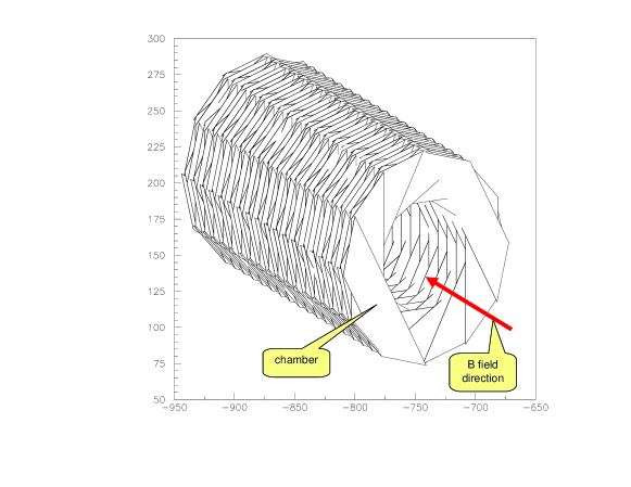
Figure 1: Schematic drawing of the tracker design.

A tracker plane consists of two trapezoidal straw tube chambers (see Fig. 1). The planes are distributed uniformly over the length of the tracker. Rotating consecutive planes by an angle of 30^o gives an effective “stereo” of crossed directions for 12 different views. Each chamber consists of one layer of straw tubes (60 straws) of 5 mm diameter. The straws are assumed to have wall thickness 25 $\mu$m and are constructed of kapton. Isobutane (C₄H₁₀) gas is assumed to fill the tubes. The tracker design allows changing the central zone radius, by moving the chambers closer to or further from the central axis, and changing the number of chambers along the tracker axis. This is needed to meet the different requirements for registration of electrons or positrons in the final state of each lepton flavor violation experiment.

Two tracker chamber layouts and magnetic field configurations are studied: one for the $\mu\to e$ conversion process and the second for $\mu\to e+\gamma$ and $\mu\to e+e+e$ processes. The first tracker layout contains 108 planes and has the central zone radius of 38 cm. The second tracker layout contains 54 planes and has the central zone radius of 10 cm. The tracker length for both layouts is the same, 300 cm. In the two layouts the tracker is immersed in a magnetic field of 1 T and 0.5 T, respectively.

3 Pattern recognition

Track reconstruction in lepton flavor violation experiments faces a significant amount of background hits in a tracker because of the high beam intensity needed to detect rare processes. A two stage procedure was developed to provide the pattern recognition in the tracker and to suppress background hits. At the first stage of pattern recognition only information on the centers of hit straws is used. The result of this stage is a significant suppression of background hits. Also, an approximate helix fitted to the straw hit centers is found and used in the next stage of pattern recognition. To improve the suppression of background hits the second stage of pattern recognition uses drift time. A deterministic annealing filter DAF [5, 6] is applied at the second stage. The DAF effectively suppresses backgrounds by dealing simultaneously with multiple competing hits.

3.1 Pattern recognition without drift time information

A detailed pattern recognition and tracker reconstruction study was done for monochromatic electrons of 105 MeV from the $\mu\to e$ conversion process in the presence of background hits. In a uniform magnetic field the trajectory of a charged particle is a helix described by 5 parameters. The construction of the tracker allows significant simplification of the initial step of the pattern recognition by reducing the problem to two dimensional tracker views. Twelve tracker views are formed by planes through the tracker axis normal to the straws. In a typical event, a two-dimensional projection of the helical trajectory, a sine curve, is observed in a few views. There are approximately 10 hits in each view, and 30 hits in the average in the event. The average number of background hits is 300 per event, which corresponds to an average straw hit rate of about 800 kHz. The hits are grouped in lobes (see Fig. 2) with a typical gap between lobes of about 70 cm. As seen in Fig. 2 the sensitive area of the tracker measures a small part of a track, but combining hits from two lobes significantly improves the precision of the momentum reconstruction.

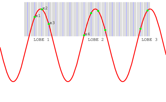
Figure 2: Lobes in the tracker view. Points show straw hit centers. The sinusoidal projection of a helix is shown in red. The starting point of the track is not shown in the figure.

The sinusoidal projection of a helix in each view is described by four parameters: $x_{0}^{\prime}$ , $z_{0}^{\prime}$, $P_{L}$, $P_{T}$,

$$x_{i}^{\prime}=x_{0}^{\prime}+aP_{T}\cos(\frac{z_{i}-z_{0}^{\prime}}{aP_{L}})$$ (1)

where $P_{L}$ and $P_{T}$ are the longitudinal and transversal momenta. The constant a equals 1/(2.998 $B$), where $B$ is the magnetic field measured in Tesla. The coordinate $z$ is common to all projections. Parameters $x_{0}^{\prime}$ and $z_{0}^{\prime}$ are defined for each given view such that the particle is created at the target with coordinate ($x_{0}^{\prime}+aP_{T}$, $z_{0}^{\prime}$).

The reconstruction algorithm starts from a single tracker view. Four hits from this view are used to give a set of equations for helix parameters in the coordinate system related to that view. The system of four equations is solved to get the parameters $P_{L},P_{T},z_{0}^{\prime},x_{0}^{\prime}$ [7]. All possible four hit combinations are considered. Only the combinations that survive a cut-off in the particle momentum ($\pm 20\%$ of the expected value) are retained for subsequent analysis.

Adding a fifth hit from a different view than the four hit combination allows defining a helical 3-D trajectory for the five-hit combination.

The following approach is used to select signal hits. If we select a combination with five signal hits the defined helical trajectory should correlate in space with other signal hits. For further analysis a five-hit combination is selected if the helical trajectory matches at least 15 additional hits in the road ($\pm$1 straw). A hit is rejected if it is not in any selected five-hit combinations. Due to the strong spatial correlations between the signal hits in comparison with the un-correlated background hits, the number of background hits is reduced drastically by applying this road requirement. A fit is applied to reconstruct an average helical trajectory on the basis of the list of the selected tracker hits. This fit does not take into account multiple scattering.

At the first stage of pattern recognition procedure the overall background rejection factor is about 130. The electron momentum from the $\mu\to e$ conversion process can be reconstructed in this stage with a standard deviation $\sigma_{p}$ = 0.45 MeV corresponding to relative momentum resolution $\sigma_{p}/p=0.5\%$.

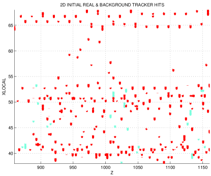
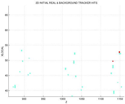
Figure 3: Plot of signal (blue dots) and background (red dots) tracker hits before (left) and after the pattern recognition procedure without drift time (right).

Figure 3 shows the multiple view superposition of tracker hits for the sample event with 29 signal and 260 background hits before and after the pattern recognition procedure. There are no missed signal hits and two surviving background hits in this case.

3.2 Kalman filter application to track reconstruction

The Kalman filter (KF) [8, 9] addresses the general problem of trying to estimate at different points ($1\leq k\leq n$) the state $\bf{x}_{k}$ of a discrete process that is governed by the linear stochastic difference equation

$$\bf{x}_{k}=\bf{F}_{k-1}\bf{x}_{k-1}+\bf{w}_{k-1}$$ (2)

with a measurement $\bf{m}_{k}=\bf{H_{k}}\bf{x}_{k}+\bf{\varepsilon}_{k}$. In the system of equations (2) stochastic processes such as multiple scattering and bremsstrahlung are taken into account by the process noise $\bf{w}_{k}$. The measurement noise is represented by $\bf{\varepsilon}_{k}$. $\bf{Q}_{k}$ and $\bf{V}_{k}$ are process noise and measurement noise covariances, respectively. In the absence of the last term Eq.(2) is the standard equation of motion with a propagator $\bf{F}_{k-1}$ (transport matrix). The $\bf{F}$ matrix propagates the state vector on one measurement plane to the state vector on the next plane combining position information with directional information.

For a particle moving in a uniform magnetic field (see Fig. 1) one has to choose the state vector parameters, define the initial state vector and calculate the transport matrix $\bf{F}$, the projection matrix $\bf{H}$, and the noise matrix $\bf{Q}$. The state vector can be chosen in the form ${\bf{x}_{k}}=(x,y,t_{x},t_{y},1/p_{L})$ where $x,y$ are the track coordinates in the tracker system, and $t_{x}=p_{x}/p_{L}$, $t_{y}=p_{y}/p_{L}$ define the track direction. The projection matrix is given by ${\bf{H}}=(\cos\alpha,\sin\alpha,0,0,0)$, where $\alpha$ is a tracker view angle.

Due to multiple scattering the absolute value of electron momentum remains unaffected, while the direction is changed. This deflection can be described using two orthogonal scattering angles, which are also orthogonal to the particle momentum [10]. In terms of these variables the noise matrix is given by

$$\bf{Q}_{k}=<\Theta^{2}>(t_{x}^{2}+t_{y}^{2}+1)\left.\left(\begin{array}[]{ccccc}0&0&0&0&0\\ 0&0&0&0&0\\ 0&0&t_{x}^{2}+1&t_{x}t_{y}&t_{x}/p_{L}\\ 0&0&t_{x}t_{y}&t_{y}^{2}+1&t_{y}/p_{L}\\ 0&0&t_{x}/p_{L}&t_{y}/p_{L}&\frac{(t_{x}^{2}+t_{y}^{2})}{p_{L}^{2}(t_{x}^{2}+t_{y}^{2}+1)}\end{array}\right.\right)$$

For the variance of the multiple scattering angle the well-known expression is used

$$<\Theta^{2}>=(p_{0}/p)^{2}[1+0.038\ln(t/X_{R})]t/X_{R}$$

where $p_{0}=$ 13.6 MeV, $X_{R}$ is a radiation length and t is a distance traveled by the particle inside a scatterer. Energy losses are taken into account by

$$p\prime=p-<dE/dx>t.$$

There are three types of operations to be performed in the analysis of a track. Prediction $\bf{x}_{k}^{k-1}$ is the estimation of the “future” state vector at position $``k"$ using all the “past” measurements up to and including $``k-1"$.

Filtering $\bf{x}_{k}^{k}$ is the estimation of the state vector at position $``k"$ based upon all “past” and “present” measurements up to and including $``k"$. At each step the filtered $\chi^{2}$ is calculated. The total $\chi^{2}$ of the track is given by the sum of the $\chi_{k}^{2}$ contributions for each plane.

Smoothing $\bf{x}_{k}^{n}$ is the estimation of the “past” state vector at position $``k"$ based on all $``n"$ measurements taken up to the present time. The filter runs backward in time updating all filtered state vectors on the basis of information from all n planes. The mathematical equations describing these operations are given in [8, 9].

The prediction and filtering are applied consecutively to all points. When the last point is reached the smoothing is applied to all previous points. The result of smoothing is a reconstruction of the state vector $\bf{x}_{k}^{n}$ which defines particle coordinates and momentum in each plane. The KF approach described above works for a single point in each plane. Background hits create multiple competitive point in each plane. In this case a different approach based on the KF will be applied as described below.

3.3 Pattern recognition with drift time

The second stage in the pattern recognition procedure uses the hits selected and fitted helix obtained in the first stage and adds drift time information for the selected hits. The pattern recognition procedure can be improved by taking into account the measured drift time $t_{i}^{meas}$ which is related to the radial distance r at the closest approach to the straw wire. The errors ($\sigma$) in radius measurements are taken to be 0.2 mm. This radius r carries an ambiguity as to whether the track passed left or right of the wire. Left and right points are extracted from the intersections of a normal to the helix through the straw center and the circle of the radius r.

A deterministic annealing filter (DAF) [5, 6] is applied to suppress background hits further. The DAF is a Kalman filter with re-weighted observations. The propagation part of DAF is identical to the standard Kalman filter. In addition to background hits a left-right ambiguity for given hit creates multiple competing points at each KF step. At the DAF step all competing points are assigned to a single layer with weights. The filtered estimate (measurement update) $\bf{x}_{k}^{k}$ at layer k is calculated as a weighted mean of the prediction $\bf{x}_{k}^{k-1}$ and the observations $\bf m_{k}^{i},i=1,2,...n_{k}$.

By taking a weighted mean of the filtered states at every layer a prediction for the state vector $\bf x_{k}^{n*}$ along with its covariance matrix $\bf{C}_{k}^{n*}$ is obtained, using all hits except the ones at layer k. Initially all assignment probabilities for the hits in each layer are set to be equal but based on the estimated state vector $\bf x_{k}^{n*}$ and its covariance matrix, the assignment probabilities of all competing hits are then recalculated in the following way:

$${\bf{p}_{k}^{i}}\sim\varphi(\bf{m}_{k}^{i};\bf{H}_{k}\bf x_{k}^{n*},\bf{V}_{k}+\bf{H}_{k}\bf{C}_{k}^{n*}\bf{H}_{k}^{T})$$

where $\varphi$ is a multivariate Gaussian probability density, $\bf{V}_{k}$ is the variance of the observations. If the probability falls below a certain threshold, the hit is considered as background and is excluded from the list of the hits assigned to the track. At the initial step we cannot be sure of calculated probabilities due to insufficient information for the filter. This problem is overcome by adopting a simulated annealing iterative procedure [5, 6] which allows avoiding a local minimum and finding the global one corresponding to the minimum chi-square for the track. The annealing schedule is chosen for the iteration n in the form ${\bf V_{n}}={\bf V}(1+\frac{C}{f^{n}})$ where the annealing factor $f>1$ and constant $C\gg 1$. This insures that the initial variance is well above the nominal value ${\bf V}$ of the observation error but the final one tends to ${\bf V}$. After each iteration the assigned probabilities exceeding the threshold are normalized to 1 and used again as weights in the next iteration, and so on. The iterations generally are stopped if the relative change in chi-square is less than a corresponding control parameter (typically of the order 0.01). Since we are dealing with a stochastic process, the best result can be reached repeating the DAF procedure for a few different annealing factors f (1.4 and 2) and then choosing the result corresponding to the minimum chi-square.

The application of the DAF procedure mainly allows resolving the left-right ambiguity. The DAF chooses wrong left-right points for 6$\%$ of the tracker hits if the radial distance r at the closest approach to the straw wire is greater then 0.25 mm. This corresponds to an average two tracker hits with the wrong left-right assignment per event. The number of background hits remaining after the second stage averages 0.38 hits per event in comparison with the primary 300 hits on average. The final background suppression factor is thus 300/0.38 $\approx$ 800. Some of the signal hits are lost due to the selection (0.8 hits or 2.7$\%$ per event on average). The momentum resolution of the tracker after application of the DAF procedure is 0.25 MeV for the $\mu\to e$ conversion process. The pattern recognition procedure described above is thus effective in the rejection of background hits and also provides a good starting point for the track reconstruction. However, further improvement in the left-right assignment is necessary to achieve better resolution. For this we use the procedure described in the following section.

4 Momentum reconstruction for the $\mu\to e$ conversion process

The momentum reconstruction is based on the hits selected by the two stage pattern recognition procedure described above. For straw drift tubes there is a set of left and right point for each straw hit due to the left-right ambiguity. An extreme possibility would be to apply the Kalman filter to all possible $2^{N}$ combinations to reconstruct a track with N hits and to choose the combination with the best $\chi^{2}$. This pure combinatorial approach may be the best but it is computationally unfeasible. The other extreme could be to apply the Kalman filter at each step to left and right points and to select the point providing the best $\chi^{2}$. However this algorithm often selects wrong points.

It has been proposed in the literature [5, 6] to use a Gaussian sum filter (GSF) for solving the assignment problem in a track detector with ambiguities [11]. In the GSF approach [12], both process noise and observation errors are modeled by a mixture of Gaussian densities and in the resulting algorithm several Kalman filters run in parallel. However the application of GSF as a momentum reconstruction procedure to this tracker does not provide sufficiently good results because of large gaps in the measured trajectory. In the tracker hits are distributed approximately uniformly inside lobes in the z-direction, but there are large gaps about 70 cm between lobes due to the motion of the electron outside the sensitive area of the tracker. A Kalman filter prediction step corresponding to a gap often leads to significant deviations from the true hit. As a result, in the GSF procedure the true component often is suppressed so significantly that it can not be recovered by subsequent Kalman filter steps. Therefore we need a different approach to treat the left-right ambiguity in the tracker.

A combinatorial drop filter (CDF) has been developed to improve the momentum reconstruction and efficiency for the tracker. The CDF algorithm uses forced minimization of the number of combinations when it reaches some maximum. So in the CDF approach the number of combinations always oscillates between $N_{min}$ and $N_{max}$. That means that the Kalman filter runs with paths increasing in number with the combinatorial growth of combinations, but each time the number of combinations reaches $N_{max}$, only the $N_{min}$ combinations with the best $\chi^{2}$ are retained. The CDF approach is illustrated by the graph $N_{min}$$\rightarrow$$N_{max}$ (2$\rightarrow$8) in Fig. 4. Each vertex represents either a left or right point. Components surviving after the drop are indicated by small (magenta) circles. In the actual strategy the number of retained components was chosen to be 8 and the maximum number of components to be 32.

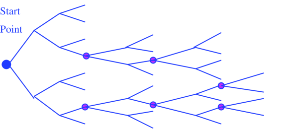
Figure 4: Graph 2$\rightarrow$8 for CDF procedure.

The procedure begins with the first eight straw hits and builds $2^{8}$ (256) possible hit combinations corresponding to left-right points. The Kalman filter forward and backward procedures are applied to these combinations. Only a few combinations which satisfy a rather loose $\chi^{2}$ cut, are retained. This step provides a certain precision for state-vector components. Each retained combination containing 8 points provides a starting point for the CDF.

The Kalman filter reconstructs a trajectory of a particle in three dimensions. The trajectory is bent each time it crosses a tracker plane due to multiple scattering. Therefore, the reconstructed track is a set of helices that intersect at the planes. Fig. 5 shows the 3D trajectory reconstructed for a sample event.

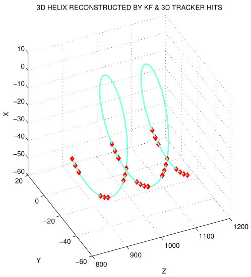
Figure 5: The 3D trajectory reconstructed for a sample event.

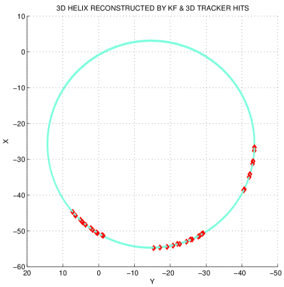
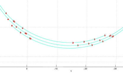
Figure 6: The transverse projection of the 3D trajectory reconstructed for a sample event (left). Enlargement of the bottom part of the trajectory (right).

On this scale the trajectory looks like a helix, but it consists of many helix parts. Fig. 6 (left) shows the transverse projection of the trajectory for the sample event. In this projection the trajectory looks approximately like a circle. However if a specific region of Fig. 6 (left) is magnified one can see in Fig. 6 (right) that the shape of the circle is distorted due to multiple scattering and energy loss. Three arcs of the trajectory are clearly seen in the Figure.

There are two main tracker reconstruction features: momentum and angle resolutions. The momentum resolution is defined from the distribution of the difference between simulated and reconstructed momentum. The angle resolution is defined from the distribution of the angle between simulated and reconstructed momentum.

In this study $10^{5}$ events were simulated and reconstructed. The CDF procedure chooses wrong left-right points for 4$\%$ of the tracker hits (to be compared with 6$\%$ for the DAF) if the radial distance r at the closest approach to the straw wire is greater then 0.25 mm. The distribution of the difference between the initial momentum reconstructed by the Kalman filter and the simulated initial momentum is shown in Fig. 7 (left) for the $\mu\to e$ conversion process. According to this distribution the intrinsic tracker resolution is $\sigma$ = 0.17 MeV if one fits the distribution by a Gaussian. Note that this tracker resolution is by about 30$\%$ better than the resolution provided by the DAF procedure.

The distribution of the angle between the reconstructed and simulated momenta is shown in Fig. 7 (right). The most probable value of the angle distribution is 3 mrad. A calculation gives an average angle of multiple scattering in a straw to be 1.8 mrad for the $\mu\to e$ conversion process. This is consistent with the expectation that the angular resolution is defined by multiple scattering in a single tracker straw.

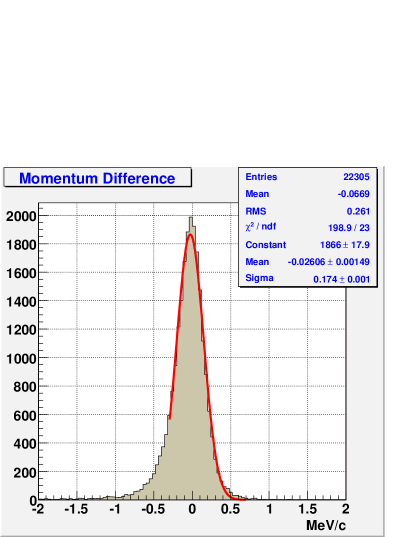
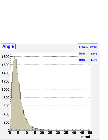
Figure 7: Reconstruction for $\mu\to e$ conversion process. The distribution of the difference between the reconstructed and simulated momentum (left). The distribution of the angle between the reconstructed and simulated momentum (right).

4.1 Momentum reconstruction for the $\mu^{+}\to e^{+}+\gamma$ process

As mentioned in the introduction, this study and the one in the next section are less complete than that carried out for the $\mu\to e$ conversion process. No background hits were added to simulated events. The second tracker layout and field configuration were used for the momentum reconstruction study of the $\mu^{+}\to e^{+}+\gamma$ process without background. The tracker is placed in a magnetic field of 0.5T which is half that used for the $\mu\to e$ conversion setup. The $\mu\to e$ conversion and the $\mu^{+}\to e^{+}+\gamma$ processes have monochromatic charged leptons in the final state whose energies differ by a factor of 2. Due to the twofold change in the magnetic field the charged lepton trajectories for the $\mu^{+}\to e^{+}+\gamma$ and the $\mu\to e$ conversion processes are similar. The pattern recognition and momentum reconstruction procedures described above were applied to positrons of the $\mu^{+}\to e^{+}+\gamma$ process. The distribution of the difference between the initial momentum reconstructed by the Kalman filter and the simulated initial momentum is shown in Fig. 8 (left). Fitting this distribution to a Gaussian gives an intrinsic tracker resolution of $\sigma$ = 0.26 MeV. The distribution of the angle between the reconstructed and simulated momentum is shown in Fig. 8 (right). The most probable value of the angle distribution is 5 mrad. A calculation gives an average angle of multiple scattering in a straw to be 3.6 mrad for a positron in the $\mu^{+}\to e^{+}+\gamma$ process.

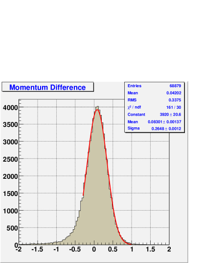
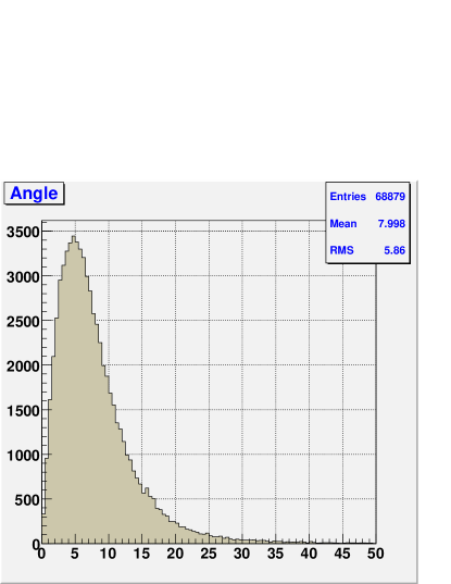
Figure 8: Reconstruction for the $\mu^{+}\to e^{+}+\gamma$ process: The distribution of the difference between the reconstructed and simulated momentum (left). The distribution of the angle between the reconstructed and simulated momentum (right).

4.2 Momentum reconstruction for the $\mu\to 3e$ process

The same setup as for the $\mu^{+}\to e^{+}+\gamma$ process was used for a momentum reconstruction study of the $\mu^{+}\to e^{+}+e^{+}+e^{-}$ process. This process has in the final state an electron and two positrons with energies from 0 to $m_{\mu}$/2 and an average energy equal to one third of the muon mass. The pattern recognition and momentum reconstruction procedure applied for $\mu\to e$ conversion and $\mu^{+}\to e^{+}+\gamma$ processes was based on a single track search algorithm. The same procedure was applied separately for each lepton track of the $\mu^{+}\to e^{+}+e^{+}+e^{-}$. The observable quantity of the process, total scalar momentum of charged leptons $p_{tot}=\sum{p_{i}}$, was reconstructed.

The distribution of the difference between reconstructed total scalar momentum and muon mass is shown in Fig. 9 (left). Fitting this distribution by a Gaussian gives a tracker resolution for total scalar momentum of $\sigma$ = 0.33 MeV. The distribution of the angle between the reconstructed lepton momentum and the simulated momentum is shown in Fig. 9 (right). The most probable value of the angle distribution is 7 mrad. A calculation gives an average angle of multiple scattering in a straw to be 5.4 mrad for charged lepton momentum equals $m_{\mu}$/3.

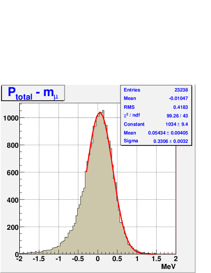
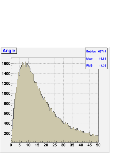
Figure 9: Reconstruction for the $\mu\to 3e$ process: The distribution of the difference between reconstructed total scalar momentum and muon mass (left). The distribution of the angle between the reconstructed and simulated momentum (right).

5 Conclusion

A pattern recognition and momentum reconstruction procedure based on a Kalman filter technique for a straw tube tracker was developed to suppress background and reconstruct track momentum for the lepton flavor violating processes $\mu\to e$ conversion, $\mu^{+}\to e^{+}+\gamma$ and $\mu\to 3e$. The simple modular construction of the tracker allows meeting requirements for lepton momentum measurements for all lepton flavor violation processes mentioned above.

The pattern recognition procedure allows suppressing the background hits by a factor of 800. Only 3% of signal hits are lost by this procedure.

The momentum resolution of the tracker to register monochromatic leptons was found to be $\sigma_{p}=$0.17 and 0.26 MeV for the $\mu\to e$ conversion with background and the $\mu^{+}\to e^{+}+\gamma$ processes without background, respectively. The tracker resolution for the total scalar lepton momentum is $\sigma_{p}=$ 0.33 MeV for the $\mu\to 3e$ process without background. For the $\mu\to e$ conversion, $\mu^{+}\to e^{+}+\gamma$ and $\mu\to 3e$ processes the most probable values of an angle between the simulated and reconstructed momenta (3, 5 and 7 mrad) are in a good agreement with multiple scattering angles in a single tracker straw. The obtained tracker resolutions allow an increase in sensitivity to the branching ratios for these processes by a few orders of magnitude over current experimental limits.

We wish to thank A. Mincer and P.Nemethy for fruitful discussions and helpful remarks. This work has been supported by the National Science Foundation under grants PHY 0428662, PHY 0514425 and PHY 0629419.

References

- [1] J.D.Vergados, Phys.Rep. 133, 1, (1986).
- [2] Y.Kuno and Y.Okada, Rev.Mod.Phys.73, 151 ,(2001).
- [3] R.M.Djilkibaev and V.M.Lobashev, Sov.J.Nucl.Phys. 49, 384, (1989).
- [4] GEANT3 CERN Program Library W5013, CERN (1984).
- [5] R. Frühwirth and A. Stradlie, Comp.Phys.Comm. 120, 197, (1999).
- [6] A. Stradlie and R. Frühwirth, Nucl.Instr.Meth. A 566, 157, (2006).
- [7] R.Djilkibaev and R.Konoplich, arXiv:hep-ex/0312022v1 (2003).
- [8] R.E.Kalman, Transactions of the ASME: J.Basic Engineering, D82, 35, (1960).
- [9] P.Billoir, Nucl.Instr.Meth. 225, 352, (1984); R.Frühwirth, ibid. A262, 444, (1987); P.Billoir and S.Qian, ibid. A294, 219, (1990); E.J.Wolin and L.L.Ho, ibid. A329, 493, (1993).
- [10] R.Mankel, Nucl.Instr.Meth. A 395, 169, (1997).
- [11] R.Frühwirth, Comp. Phys. Communication 100, 1-16 (1997).
- [12] G.Kitagawa, Ann. Inst. Statist. Math. 46, 605 (1994).