Nonlinear resonances of Water Waves

Abstract.

In the last fifteen years great progress has been made in the understanding of nonlinear resonance dynamics of water waves. Notions of scale- and angle-resonances have been introduced, new type of energy cascade due to nonlinear resonances in the gravity water waves has been discovered, conception of a resonance cluster has been much and successfully employed, a novel model of laminated wave turbulence has been developed, etc. etc. Two milestones in this area of research have to be mentioned: a) development of the $q$-class method which is effective for computing integer points on resonance manifolds, and b) construction of marked planar graphs, instead of classical resonance curves, representing simultaneously all resonance clusters in a finite spectral domain, together with their dynamical systems. Among them, new integrable dynamical systems have been found that can be used for explaining numerical and laboratory results. The aim of this paper is to give a brief overview of our current knowledge about nonlinear resonances among water waves, and finally to formulate the three most important open problems.

Elena Kartashova

RISC, J. Kepler University

Altenbergerstr. 69

Linz, A-4040, Austria

(Communicated by the associate editor name)

1. Exposition

In this paper we will try to present a major part of known analytical, numerical and laboratory results on nonlinear resonances among water waves, in as strict mathematical language as possible. This is not a simple task due to the three-fold problem: 1) there is no strict definition of a wave; 2) there is no general agreement about the types of waves which should be called water waves; 3) the notions of resonance in physics and mathematics are different. Let us go through all these points one by one, regarding for concreteness 2D-wavevectors.

First, the simplest possible understanding of a (propagating) wave as a Fourier harmonics

$$A_{\mathbf{k}}\exp{i({\mathbf{k}}\cdot{\mathbf{x}}-\omega\,t)}$$ (1)

is obviously too simplified and does not include normal modes which are due to boundary conditions. Here $\mathbf{x}=(x_{1},\,x_{2}\,)$ and time $t$ are space and time variables correspondingly, $\omega=\omega(\mathbf{k})$ is dispersion function and $\mathbf{k}$ is wavevector. For instance, the normal mode of oceanic planetary waves (that are due to the Earth rotation) with zero boundary conditions in a finite box $[0,L_{x_{1}}]\times[0,L_{x_{2}}]$ reads [43]

$$|A_{\mathbf{k}}|\sin\!\Big{(}\pi\frac{mx_{1}}{L_{x_{1}}}\Big{)}\sin\!\Big{(}\pi\frac{nx_{2}}{L_{x_{2}}}\Big{)}\,\sin\!\Big{(}\frac{\beta}{2\omega}x_{1}+\omega t\Big{)}.$$ (2)

Boundary conditions on a sphere or a circle lead to even more complicated forms of the normal mode including special functions [43]. ”We seem to be left at present with the looser idea that whenever oscillations in space are coupled with oscillation in time through a dispersion relation, we expect the typical effects of dispersive waves” [61]. So, from now on we assume that dispersion function $\omega(\mathbf{k})$ defines the type of a wave, for instance, $\omega\sim|\mathbf{k}|^{3/2}$ corresponds to capillary waves in a rectangular box with periodic boundary conditions, $\omega\sim|\mathbf{k}|^{-1}$ corresponds to oceanic planetary waves in a rectangular box with zero boundary conditions, etc. Sign ”$\sim$” instead of ”$=$” in definitions of dispersion function means that some constant is omitted.

Second, capillary, gravity-capillary, gravity surface, oceanic planetary and freak waves, tsunami, internal waves in rotating fluid, etc., etc. can be observed in water, and they all can be – and sometimes are – called water waves. This is, of course, too extensive a definition that does not allow any reasonable overview, neither in the form of a paper nor of a book. An example of another extreme can be given by [37] where only waves on the surface of deep water are called ”water waves”. In this paper we choose to follow the classical conception of water waves [61], as defined by dispersion function

$$\omega^{2}=(g\,k\tanh k\,d)(1+\frac{\sigma}{\rho g}k^{2}),\quad\mbox{with}\quad k=|\mathbf{k}|$$ (3)

and $g,\,d,\,\sigma,\,\rho$ being the gravitational constant of acceleration, the average water depth, the coefficient of surface tension and density correspondingly. In this paper we will concentrate on, though not restrict ourselves completely by, the three limiting cases of (3) for water waves, with $\rho=1$ and $k\,d\rightarrow\infty$, which are important for numerous applications:

$$1. \quad\mbox{capillary waves,}\quad\lambda_{ch}\ll 2\,\,\mbox{cm}:\quad\omega^{2}=\sigma k^{3},$$ (4)

$$2. \quad\mbox{gravity waves,}\quad\lambda_{ch}\gg 2\,\,\mbox{cm}:\quad\omega^{2}=gk,$$ (5)

$$3. \quad\mbox{gravity-capillary waves,}\quad\lambda_{ch}\sim 2\,\,\mbox{cm}:\quad\omega^{2}=g\,k+\sigma k^{3},$$ (6)

where $\lambda_{ch}$ denotes characteristic wave length for each approximation.

Third, the notion of resonance appears in mathematics in the theory of Poincaré normal forms, as a condition of linearization of a nonlinear ODE or a system of nonlinear ODEs [42], in the form

$$p_{1}\omega_{1}+\cdots+p_{s}\omega_{s}+p_{s+1}\omega_{s+1}=0$$

where $\omega_{j}$ is notation for $\omega(\mathbf{k}_{j})$ and $p_{1},\,p_{2},\,\dots,\,p_{s+1}\in\mathbb{Z}$ are integers. The physical notion of resonance has been first introduced by Galileo Galilei [16] who studied oscillations of a pendulum under the action of a small external force. In modern language, the corresponding equation reads $x_{tt}+r^{2}x=\varepsilon\exp{(ift)}$ with $0<\varepsilon\ll 1,$ and the oscillation amplitude grows linearly with time if eigenfrequency of the system $\omega$ coincides with the frequency of the driving force $f.$ The analogy with the three-wave resonance is now obvious: two Fourier harmonics of the form (1) with wavevectors $\mathbf{k}_{1},\,\mathbf{k}_{2},$ frequencies $\omega_{1},\,\omega_{2}$ and amplitudes $A_{1},\,A_{2}$ will give resonance with harmonic

$$A_{3}\exp{[i({\mathbf{k}_{1}\pm\mathbf{k}_{2}})\cdot{\mathbf{x}}-(\omega_{1}\pm\omega_{2})\,t]},$$

which yields 3-wave resonance conditions in the form

$$\omega_{1}+\omega_{2}=\omega_{3},\quad\mathbf{k}_{1}+\mathbf{k}_{2}=\mathbf{k}_{3}.$$ (7)

Similarly, 4-wave resonance conditions read

$$\omega_{1}+\omega_{2}=\omega_{3}+\omega_{4},\quad\mathbf{k}_{1}+\mathbf{k}_{2}=\mathbf{k}_{3}+\mathbf{k}_{4}.$$ (8)

In the case of periodic or zero boundary conditions, solutions of (7),(8) have to be found in integers, i.e. for $\mathbf{k}_{j}=(m_{j},n_{j})$ with $m_{j},\,n_{j}\in\mathbb{Z}.$ Solutions of (7) and (8) are called triads and quartets correspondingly, they are defined by the geometry of the wave system and do not depend on time, that is, they describe kinematics of a wave system. Dynamics of a resonant triad is covered by

$$i\,\dot{A}_{1}={V^{3}_{12}}^{\ast}A_{2}^{\ast}A_{3},\quad i\,\dot{A}_{2}={V^{3}_{12}}^{\ast}A_{1}^{\ast}A_{3},\quad i\,\dot{A}_{3}=V^{3}_{12}A_{1}A_{2},$$ (9)

where $A_{j}$ are amplitudes of three waves satisfying (7) and $\dot{A}=\frac{d}{dT}{A}$. Dynamical system for a resonant quartet reads

$$i\,\dot{A}_{1}=T^{12}_{34}A_{2}^{\ast}A_{3}A_{4}+(\Omega_{1}-\omega_{1})A_{1}\,,\quad i\,\dot{A}_{2}=T^{12}_{34}A_{1}^{\ast}A_{3}A_{4}+(\Omega_{2}-\omega_{2})A_{2}\,,$$

$$i\,\dot{A}_{3}={T^{12}_{34}}^{\ast}A_{4}^{\ast}A_{1}A_{2}+(\Omega_{3}-\omega_{3})A_{3}\,,\quad i\,\dot{A}_{4}={T^{12}_{34}}^{\ast}A_{3}^{\ast}A_{1}A_{2}+(\Omega_{4}-\omega_{4})A_{4}\ .$$ (10)

where $\Omega_{j}$ are so-called ”Stocks-corrected” frequencies [53]. They are often omitted in the literature while suitable renormalization of $\omega$-s yields more usual form of (1), without terms $(\Omega_{j}-\omega_{j})A_{j}$ included (e.g. [38], for one-dimensional quartets). The general form of (9), (1) can be deduced in the frame of the Hamiltonian formalism, [66], and does not depend on the type of waves. The only difference between various wave types is hidden in the form of coupling coefficients $V^{3}_{12}$ and $T^{12}_{34}$; their expressions for water waves are given in the Table 1. Resonant triads and quartets may form resonance clusters, for instance when one resonant mode $(m,n)$ is part of a few solutions of (7) or (8). Obviously, triads and quartets are the minimal resonance clusters in three- and four-wave systems correspondingly; they are called primary clusters.

Remark 1.

To use the Hamiltonian formalism for describing these wave systems, some small parameter $0<\varepsilon\ll 1$ has to be introduced, which allows the application of variational or multi-scale methods. These yield, in the the simplest case, two time-scales - fast time, $t$, for the linear Fourier harmonic (1), and slow time, $T=\varepsilon\,t$, for the amplitudes of the nonlinear resonant mode (9). In water wave systems, wave steepness is usually taken as a small parameter, $\varepsilon\sim 0.1$.

2. Kinematics

2.1. Exact resonances

Computing integer solutions of resonance conditions (7), (8) for dispersion functions (4)-(5) is equivalent to finding integer points on a resonant manifold of a high degree in many variables. Loosely speaking, the problem is equivalent to Hilbert’s Tenth Problem [21], which is proven to be unsolvable in the general case [40], and even for the case of two variables only partial results are known. We are interested in solutions of equations (7), (8) with 6 and 8 variables correspondingly. One could hope that numerical search for solutions might be a reasonable possibility but it is not. Full search for multivariate problems in integers consumes exponentially more time with the size of the domain to be explored and for each additional variable. For (8) in the domain $|m|,\,|n|\sim 1000$ this would imply some $10^{24}$ tries. Still worse, the equations include radicals and straightforward transformation to a purely integer form would lead to operations with huge integer numbers - for the said domain, of the order of $10^{120}$. All these reasons make a quest for effective algorithms unavoidable.

A special method for solving systems of the form (7), (8) has been presented in [26] for gravity waves with dispersion function (5). Details of its implementation and numerical results for various irrational dispersion functions can be found in [29, 30]. The method is called $q$-class method or $q$-class decomposition. Its idea comes from the linear independence of a finite number of some algebraic numbers. Below we give the general definition of the $q$-class and show how to use it for finding solutions of (7), (8).

Definition 2.1.

For a given $c\in\mathbb{N},c\neq 0,1,-1$ consider the set of algebraic numbers $R_{c}={k^{1/c},k\in\mathbb{N}}$. Any such number $k_{c}$ has a unique representation

$$k_{c}=\gamma q^{1/c},\gamma\in\mathbb{Z}\quad\mbox{with}\quad q=p_{1}^{e_{1}}p_{2}^{e_{2}}...p_{n}^{e_{n}},$$

and $p_{1},...p_{n}$ being all different primes and the powers $e_{1},...e_{n}\in\mathbb{N}$ are all smaller than $c$. The set of numbers from $R_{c}$ having the same $q$ is called $q$-class $Cl_{q}$. The number $q$ is called class index.

Now we can decompose the computational domain into $q$-classes and search for solutions in each class separately. The computational advantage of using $q$-class decomposition is huge. For instance, for dispersion function (5) and resonance conditions (8) straightforward computation takes 3 days with Pentium-4 in the spectral domain $|m|,|n|\leq 128$; the $q$-class decomposition produces all solutions for $|m|,|n|\leq 1000$ in about 15 minutes with Pentium-3.

2.1.1. Capillary waves, $\omega^{2}=\sigma k^{3},$ three-wave resonances.

In this case, we take $c=2$ in the definition above and represent the norm $k_{j}$ as

$$k_{j}=\gamma_{j}\sqrt{q_{j}},\quad\gamma_{j},\,q_{j}\in\mathbb{N},\quad q_{j}\quad\mbox{is square-free}$$ (11)

The presentation (11) is unique for each $k_{j}$ and it follows that

$$\omega_{1}+\omega_{2}=\omega_{3}\quad\ \Rightarrow\ \quad\gamma_{1}^{3}q_{1}\sqrt{q_{1}}+\gamma_{2}^{3}q_{2}\sqrt{q_{2}}=\gamma_{3}^{3}q_{3}\sqrt{q_{3}}.$$ (12)

The necessary condition of the existence of integer solutions of (12) is $q_{1}=q_{2}=q_{3},$ say $q_{j}=q,\,\forall j=1,2,3,$ (see [25]), and this allows to reduce (12) to a particular case of Fermat’s Last Theorem, $\gamma_{1}^{3}+\gamma_{2}^{2}=\gamma_{3}^{3},$ i.e. there are no resonances among capillary waves with dispersion function (4).

The case of capillary waves is unique. Usually, a three-wave system possesses a number of resonances divided into small resonance clusters [24]. Mostly, resonance clusters are isolated triads or groups of two connected triads ($70-100\%\%$ of all clusters, depending on the size of the spectral domain). For instance, the same $q$-class construction used for ocean planetary waves with dispersion function $\omega\sim k^{-1/2}$ and resonance conditions (7), turns the first equation of (7) into $\gamma_{2}\,\gamma_{3}+\gamma_{1}\,\gamma_{3}=\gamma_{1}\,\gamma_{2},$ in which case solutions do exist [29].

At the end of this section we would like to mention quite recent progress on the resonances of capillary waves reported in [8]. Dispersion function has been taken in the form

$$\omega=\frac{\Omega}{2}+\frac{1}{2}\sqrt{\Omega^{2}+4k^{3}\sigma},$$ (13)

where $\Omega$ is non-zero constant vorticity. The main results are as follows: 1) wave trains in flows with constant non-zero vorticity are possible only for two-dimensional flows; 2) only positive constant vorticities can trigger the appearance of three-wave resonances; 3) the number of positive constant vorticities which do trigger a resonance is countable; 4) the magnitude of positive constant vorticity triggering a resonance can not be too small. Of course, these results are only valid for waves with small amplitude [8, 9, 10, 60] (cf. Remark 1 above).

2.1.2. Gravity-capillary waves, $\omega^{2}=g\,k+\sigma k^{3},$ three-wave resonances.

Construction of $q$-classes is this case differs from (11) and is more intricate [32], due to the fact that dispersion function contains two irrationalities and is not homogenous on $k,$ i.e. coefficients $g$ and $\sigma$ do not disappear. For numerical simulations, we used $g=981$ and two values of $\sigma$: $\sigma=74$ and $\sigma=75$, for water with temperature $18^{\circ}$C and $8^{\circ}$C correspondingly. Numerical simulations have been performed, seeking solutions $\omega_{1}+\omega_{2}=\omega_{3}(1+\varepsilon)$, for various $\varepsilon,$ $0\leq|\varepsilon|\leq 10^{-4}$. Spectral domain $-100\leq m,\,n\leq 100$ has been investigated. For both cases, $\sigma=74$ and $\sigma=75$, only isolated triads have been found (for $\varepsilon=0$): 24 and 16 triads correspondingly; no triad appears simultaneously in both lists. The resonance structure is much richer for $\varepsilon>0,$ resonance clusters of two to six triads appearing already for $\varepsilon=10^{-7}$, while for $\varepsilon=10^{-4}$ the overall number of resonances is about $10^{6},$ and more than $90\%$ of all resonant triads coincide for $\sigma=74$ and $\sigma=75$.

2.1.3. Gravity waves, $\omega^{2}=gk,$ four-wave resonances.

In this case, $c=4$ in the definition of the $q$-class, i.e. $k=(m^{2}+n^{2})^{1/4}=\gamma q^{1/4}$, where $q$ does not contain fourth degrees in its representation as a product of different primes in corresponding powers [26]. It can be proven that only two cases are possible: 1) all 4 wavevectors, forming a solution of (8), belong to one class $Cl_{q}$, and 2) two wavevectors belong to $Cl_{q_{1}}$ and two others belong to $Cl_{q_{2}}$ with $q_{1}\neq q_{2}.$ Again, this is only a necessary, not a sufficient condition for the existence of a solution.

From physical point of view, the main difference between nonlinear resonances in three- and four-wave systems can be formulated as follows. Any three-wave resonance generates a new frequency and, correspondingly, new wave length, i.e. any three-wave resonance contributes to the energy transfer over the scales. This is not true in four-wave systems. Indeed, let us regard one specific solution of (8): $\mathbf{k}_{1}=(-64,-16),\,\mathbf{k}_{2}=(4,16),\,\mathbf{k}_{3}=(-64,16),\,\mathbf{k}_{4}=(4,-16).$ This solution is not trivial - all wavevectors are different, but $k_{1}=k_{3}$ and $k_{2}=k_{4},$ i.e. no new wave length appears due to this kind of resonances. Being regarded in $\mathbf{k}$-space, these resonances perform the energy transfer not over the scales but over the angle, forming two circles. Correspondingly, two types of resonances are singled out, with different dynamics - angle- and scale-resonance [28].

The fact of utmost importance is that these two types of resonances should not be studied separately, because mixed cascades also exist. For instance, the wavevector (119,120) takes part in one scale-resonance and 12 angle-resonance [28]. Complete study of all the resonances in the spectral domain $|m_{i}|,|n_{i}|\leq 1000$ can be found in [35]. In this domain, there are more than 600.000.000 exact resonances, among them only 230.464 angle-resonances, among which 213.760 resonances are formed by four collinear wavevectors. As it is shown in [14], the coupling coefficient (see Table 1) in this case is equal to zero, i.e. these resonances do not affect dynamics. Some parametric series of solutions for the resonance conditions (8) are known, for instance, for any given wavevector $(m,n),$ a 3-parametric series of angle-resonances is known:

$${\bf k}_{1}=(m,n),\ {\bf k}_{2}=(t,-n),\ {\bf k}_{3}=(m,-n),\ {\bf k}_{4}=(t,n),\quad t=0,\pm 1,\pm 2,\ldots.$$ (14)

Series of scale-resonances called tridents has been first found in [39] for quartets of the form:

$${\bf k}_{1}=(a,0),\ {\bf k}_{2}=(-b,0),\ {\bf k}_{3}=(c,d),\ {\bf k}_{4}=(c,-d)\,,$$ (15)

where $a=(s^{2}+t^{2}+st)^{2},\ b=(s^{2}+t^{2}-st)^{2},\ c=2st(s^{2}+t^{2}),\ d=s^{4}-t^{4}\,,s,t\in\mathbb{N}.$ This series is of special interest for studying large-scale gravity waves: all scale-resonances in the spectral domain, say, $k\leq 100$ are of this form [35] and therefore can be found analytically. Analytical series are very helpful not only for computing resonance quartets and cluster structure but also for investigating the asymptotic behavior of coupling coefficients. More details can be found in [35].

Remark 2.

The results reported in this section were possible to obtain because all three dispersion functions (4)-(5) are irrational and we could make use of the $q$-class method. Interestingly enough, similar idea can also be worked out into a computational method for a transcendental dispersion function, say, $\omega^{2}=g\,k\tanh k\,d.$ Indeed, using standard presentation $\tanh x=[\exp{x}-\exp{(-x)}]/[\exp{x}+\exp{(-x)}],$ one can rewrite (8) as a combination of different exponents with polynomial coefficients depending on $k$ and $d$ (see [23], Discussion, p.52). Afterwards appropriate theorems about linear independence of exponents over algebraic numbers can be used [2]. This procedure can be used for any transcendental dispersion function which has a representation as a rational function of different exponents.

2.2. Topological structure of the complete resonance set

In 1950-1960th the usual way to represent nonlinear resonances was to construct a resonance curve that is the locus of pairs of wavevectors interacting resonantly with a given wavevector. A locus might be an ellipse, be shaped like an hour-glass, can degenerate into a pair of lines, etc. Eventually, the characteristic form of the locus is useful to know before planning some laboratory experiments: in [45] a resonance curve has been constructed for a special type of resonant quartets of gravity waves, in which two wavevectors coincide. A typical resonance curve for gravity-capillary waves can be found in [46]. The main drawback of the resonance curve presentation is that it allows to visualize – at most – only a part of the resonance set. And of course, without the $q$-class method, there has been no constructive way to establish whether any integer points exist on these curves.

A novel graphical presentation of 2D-wave resonances as a planar graph, [34], provides a very clear and transparent way to exhibit the complete resonance set. The construction is performed in two steps. First, each 2D-vector is regarded as a node of integer lattice in the spectral space, and nodes which construct one solution (triad or quartet) are connected. The result is called geometrical structure of the resonance set and can be rather nebulous [34]. Second, all different topologically equivalent components of the graph, corresponding to the geometrical structure, are singled out. The list of all these elements together with a number, showing how many times a specific component is met in the solution set, is called topological structure of the resonance set. For instance, in a three-wave resonance system, most part of the elements are either isolated triads, shown as triangles, or butterflies, shown as two triangles with one joint vertex. For dynamical reasons which are explained in the Sec. 3.2, it is important to known whether or not a connection within a cluster is realized via a mode with maximal frequency ($\omega_{3}$-mode). This mode is marked by the letter A in each triangle, while two other modes are marked by P. Examples of topological elements appearing in the various water wave systems are shown in Fig.1 in Sec. 3.2. This construction can be extended to the case of four wave resonances but the structure of clusters is more involved [35].

3. Dynamics

3.1. Primary clusters

A more compact form of (9) can be obtained by a suitable change of variables and reads

$$\dot{B}_{1}=ZB_{2}^{*}B_{3},\quad\dot{B}_{2}=ZB_{1}^{*}B_{3},\quad\dot{B}_{3}=-ZB_{1}B_{2}.$$ (16)

It has three conservation laws (e.g. [4])

$$I_{23}=|B_{2}|^{2}+|B_{3}|^{2},\ I_{13}=|B_{1}|^{2}+|B_{3}|^{2},\ H_{tr}=\operatorname{Im}(B_{1}B_{2}B_{3}^{*}).$$ (17)

The first two of them, $I_{23}$ and $I_{13},$ can be rewritten via energy and enstrophy, while the last one $H_{tr}$ is the Hamiltonian of the triad. Notice that though (16) has 3 complex variables, i.e. 6 real variables, and only three conservation laws, it is easy to show that it is integrable. Indeed, one should rewrite it in the standard amplitude-phase representation $B_{j}=C_{j}\exp(i\theta_{j})$:

$$\dot{C}_{1}=ZC_{2}C_{3}\cos\varphi,\quad\dot{C}_{2}=ZC_{1}C_{3}\cos\varphi,\quad\dot{C}_{3}=-ZC_{1}C_{2}\cos\varphi,$$ (18)

$$\dot{\varphi}\ =-Z\,H_{tr}(C_{1}^{-2}+C_{2}^{-2}-C_{3}^{-2}).$$ (19)

where $\varphi=\theta_{1}+\theta_{2}-\theta_{3}$ is called dynamical phase. Now the four equations (18),(19) have four real variables, and analytical expressions for amplitudes $C_{1},\,C_{2},\,C_{3}$ are found in Jacobian elliptic functions $\mathbf{dn},\,\mathbf{sn},\,\mathbf{cn}$ [62]. Using relations between squares of elliptic functions, we can represent squared amplitudes as

$$\begin{cases}C_{1}^{2}(T)=-\mu\,\left(\frac{2K(\mu)}{Z\,\tau}\right)^{2}{{\mathbf{sn}^{2}}\left(2\,K(\mu)\,\frac{{(T-t_{0})}}{{\tau}},\mu\right)}+\gamma_{1}\\ C_{2}^{2}(T)=-\mu\,\left(\frac{2K(\mu)}{Z\,\tau}\right)^{2}{{\mathbf{sn}^{2}}\left(2\,K(\mu)\,\frac{{(T-t_{0})}}{{\tau}},\mu\right)}+\gamma_{2}\\ C_{3}^{2}(T)=\ \mu\,\left(\frac{2K(\mu)}{Z\,\tau}\right)^{2}{{\mathbf{sn}^{2}}\left(2\,K(\mu)\,\frac{{(T-t_{0})}}{{\tau}},\mu\right)}+\gamma_{3}\,,\end{cases}$$ (20)

where $K(\mu)$ is elliptic integral of the first order, and $\mu,\,t_{0},\,\tau,\,\gamma_{1},\,\gamma_{2},\,\gamma_{3}$ are explicit rational expressions of the initial values of the amplitudes $C_{1}^{2}(0),C_{2}^{2}(0),C_{3}^{2}(0)$ (see [6]). Since the energy of each mode $E_{j}$ is proportional to its squared amplitude $C_{j}^{2}$ and $0\leq\mathbf{sn}^{2}\leq 1,$ the characteristic energy variation of any resonant mode $E_{mode}\sim\mathbf{sn}^{2}(k\,t,\mu)$ is bounded: $0\leq E_{mode}\leq E_{0},$ with $E_{0}=E_{0}(I_{13},I_{23},H_{tr})$ being an explicit function of the initial conditions.

The dynamical phase satisfies an evolution equation (19) and its solution cannot be obtained by simply replacing the solution for the amplitudes in the Hamiltonian $H_{tr}=C_{1}C_{2}C_{3}\sin\varphi$ and solving for $\varphi$. The reason is that non-zero $\varphi$ generically evolves between $0$ and $\pi$, crossing the value $\varphi=\pi/2$ periodically. This implies that $\sin^{-1}$ is double-valued and thus it is not possible to obtain $\varphi$ in a unique way. Importance of the dynamical phase is due to the fact that it effects substantially the magnitudes of $C_{1},C_{2},C_{3}$ (see Fig.1 from [5]). Solution for $\varphi,$ first obtained in [6], reads

$$\varphi(t)=\textrm{sign}(\varphi_{0})\,\mathrm{\mathbf{arccot}}\left(-\frac{\mu}{|H_{tr}|}\left(\frac{2K(\mu)}{Z\,\tau}\right)^{3}\mathrm{\mathbf{sn\,cn\,dn}}\left(2\,K(\mu)\,\frac{{(T-t_{0})}}{{\tau}},\mu\right)\right)\,,$$ (21)

with notation $\mathrm{\mathbf{sn\,cn\,dn}}(x,\mu)\equiv\mathrm{\mathbf{sn}}(x,\mu)\,\mathrm{\mathbf{cn}}(x,\mu)\,\mathrm{\mathbf{dn}}(x,\mu)\,.$

Substantially less is known about the integrability of (1). Its analysis can probably be carried out along the same lines as for (9). A promising start has been made in [53], though analysis was not brought all the way to explicit formulae similar to those obtained for (9). Also the importance of the dynamical phase has not been put to work yet, while (1) is analyzed in the complex form and the effect of the dynamical phase is hidden. For the general form of a quartet and for arbitrary initial conditions, (1) ”does not exhibit strict periodicity” [53], though in the particular case of a trident, its behavior is periodic [52] (both statements refer to the results of numerical simulations).

1	2	3
$\sigma k^{3/2}$	$V^{3}_{12}$	$\quad{i\over 8\pi\sqrt{2\sigma}}\sqrt{\omega_{1}\omega_{2}\omega_{3}}\times\left[{\mathcal{K}_{k_{2},k_{3}}\over k_{1}\sqrt{k_{2}k_{3}}}-{\mathcal{K}_{k_{1},-k_{2}}\over k_{3}\sqrt{k_{1}k_{2}}}-{\mathcal{K}_{k_{1},-k_{3}}\over k_{2}\sqrt{k_{1}k_{3}}}\right]\,$
	[64]
		where $\mathcal{K}_{k_{2},k_{3}}=({\mathbf{k}}_{2}\cdot{\mathbf{k}}_{3})+k_{2}k_{3}\$.
$(g\,k+\sigma k^{3})^{1/2}$	$V^{3}_{12}$	$\quad\quad\quad\frac{(\omega_{2}^{2}-\omega_{2}\omega_{3}+\omega_{3}^{2})}{\omega_{1}}k_{1}-\omega_{2}k_{2}+\omega_{3}k_{3}$
	[41]
		$+({\mathbf{k}}_{2}\cdot{\mathbf{k}}_{3})\big{(}\frac{\omega_{2}}{k_{2}}-\frac{\omega_{3}}{k_{3}}-\frac{\omega_{2}\omega_{3}}{\omega_{1}}\frac{k_{1}}{k_{2}k_{3}}\big{)}$
$gk^{1/2}$	$T^{12}_{34}$	$\quad\quad\frac{1}{16\pi^{2}(k_{1}k_{2}k_{3}k_{4})^{1/4}}\Big{[}-12k_{1}k_{2}k_{3}k_{4}$
	[63]
		$-2\frac{(\omega_{1}+\omega_{2})^{2}}{g^{2}}[\omega_{3}\omega_{4}({\mathbf{k}}_{1}\cdot{\mathbf{k}}_{2}-k_{1}k_{2})+\omega_{1}\omega_{2}({\mathbf{k}}_{3}\cdot{\mathbf{k}}_{4}-k_{3}k_{4})]$
		$-2\frac{(\omega_{1}-\omega_{3})^{2}}{g^{2}}[\omega_{2}\omega_{4}({\mathbf{k}}_{1}\cdot{\mathbf{k}}_{3}+k_{1}k_{3})+\omega_{1}\omega_{3}({\mathbf{k}}_{2}\cdot{\mathbf{k}}_{4}+k_{2}k_{4})]$
		$-2\frac{(\omega_{1}-\omega_{4})^{2}}{g^{2}}[\omega_{2}\omega_{3}({\mathbf{k}}_{1}\cdot{\mathbf{k}}_{4}+k_{1}k_{4})+\omega_{1}\omega_{4}({\mathbf{k}}_{2}\cdot{\mathbf{k}}_{3}+k_{2}k_{3})]$
		$+4(\omega_{1}+\omega_{2})^{2}\frac{({\mathbf{k}}_{1}\cdot{\mathbf{k}}_{2}-k_{1}k_{2})(-{\mathbf{k}}_{2}\cdot{\mathbf{k}}_{4}+k_{2}k_{4})}{\omega^{2}_{1+2}-(\omega_{1}+\omega_{2})^{2}}$
		$+4(\omega_{1}-\omega_{3})^{2}\frac{({\mathbf{k}}_{1}\cdot{\mathbf{k}}_{3}+k_{1}k_{3})({\mathbf{k}}_{2}\cdot{\mathbf{k}}_{4}+k_{2}k_{4})}{\omega^{2}_{1-3}-(\omega_{1}-\omega_{3})^{2}}$
		$+4(\omega_{1}-\omega_{4})^{2}\frac{({\mathbf{k}}_{1}\cdot{\mathbf{k}}_{4}+k_{1}k_{4})({\mathbf{k}}_{2}\cdot{\mathbf{k}}_{3}+k_{2}k_{3})}{\omega^{2}_{1-4}-(\omega_{1}-\omega_{4})^{2}}$
		$+({\mathbf{k}}_{1}\cdot{\mathbf{k}}_{2}+k_{1}k_{2})({\mathbf{k}}_{3}\cdot{\mathbf{k}}_{4}+k_{3}k_{4})$
		$+(-{\mathbf{k}}_{1}\cdot{\mathbf{k}}_{3}+k_{1}k_{3})(-{\mathbf{k}}_{2}\cdot{\mathbf{k}}_{4}+k_{2}k_{4})$
		$+(-{\mathbf{k}}_{1}\cdot{\mathbf{k}}_{4}+k_{1}k_{4})(-{\mathbf{k}}_{2}\cdot{\mathbf{k}}_{3}+k_{2}k_{3})\Big{]}$

Table 1. Overall data on three types of water waves: form of dispersion function, notation for coupling coefficient and original reference, form of coupling coefficient (1st, 2d and 3d columns correspondingly).

3.2. Clusters of two and more triads

Dynamics of a cluster consisting of a few connected triads depends on whether or not the connecting mode is the mode with maximal frequency $\omega_{3}$ in one or both triads [33]. It follows from the form of conserved quantities $I_{23},I_{13}$ (see (17)) that if only one of the modes with lower frequencies $\omega_{1}$ and $\omega_{2}$ is exited, it can not share its energy with other modes. Therefore these two modes are called P-modes, P from passive. On the contrary, $\omega_{3}$-mode is called A-mode, A from active, because being exited initially, it causes exponential growth of P-modes amplitudes, until all the modes will have comparable magnitudes of amplitudes (cf. the criterium of instability in [20]). In Fig. 1 examples of simple resonance clusters are given, with marked vertexes. Each isolated marked graph defines uniquely some dynamical system. For instance, a PP-butterfly consisting of triad $a$ and triad $b$, connected via the mode $B_{1a}=B_{1b},$ is covered by

$$\dot{B}_{1a}=Z_{a}B_{2a}^{*}B_{3a}+Z_{b}B_{2b}^{*}B_{3b},\quad\dot{B}_{2a}=Z_{a}B_{1a}^{*}B_{3a},$$

$$\dot{B}_{2b}=Z_{b}B_{1a}^{*}B_{3b},\quad\dot{B}_{3a}=-Z_{a}B_{1a}B_{2a},\quad\dot{B}_{3b}=-Z_{b}B_{1a}B_{2b}\ .$$ (22)

and conservations laws have the form

$$I_{23a}=|B_{2a}|^{2}+|B_{3a}|^{2}\,,\quad I_{23b}=|B_{2b}|^{2}+|B_{3b}|^{2}\,,$$

$$I_{ab}=|B_{1}|^{2}+|B_{3a}|^{2}+|B_{3b}|^{2}\,,\quad H_{but}=\operatorname{Im}(Z_{a}B_{1}B_{2a}B_{3a}^{*}+Z_{b}B_{1}B_{2b}B_{3b}^{*}).$$

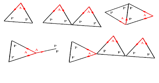
Figure 1. Triad with marked vertices; PP-butterfly; AP-PP-kite, AA-ray and AP-PP-chain of three triads.

Some scattered results on the integrability of resonance clusters can be found in [4, 6, 57, 58]. For instance, PP-butterfly (3.2) is known to be integrable if 1) $Z_{a}/Z_{b}=1$ or 2 or 1/2; and 2) $Z_{a},Z_{b}$ are arbitrary and $H_{but}=0$. However, it is not proven that this list is exhaustive. Some of the kites, rays and finite chains of triads (see Fig.1) are integrable, but complete classification of integrable resonance clusters is still to be constructed.

No quantitative results are known about dynamics of resonance clusters in four-wave systems. Simple qualitative scenario suggested in [35] is based on the pure kinematic considerations – reservoirs formed by many angle quartets in quasi-thermal equilibrium with sparse links between them formed by scale-resonances – and has yet to be justified. At least, magnitudes of coupling coefficients have to be computed; this qualitative scenario will be invalidated, for instance, if most of angle-resonances have zero coupling coefficients, or their magnitudes are substantially smaller then those of scale-resonances, etc.

Remark 3.

Three-wave system might possess a four-wave resonance cluster but it will not be a primary cluster (see Fig.1, kite or ray). This can easily be seen from the form of the corresponding dynamical system. For instance, a PP-PP kite, with $B_{1a}=B_{1b}$ and $B_{2a}=B_{2b},$ has dynamical system

$$\dot{B}_{1a}=B_{2a}^{*}(Z_{a}B_{3a}+Z_{b}B_{3b})\,,\quad\dot{B}_{2a}=B_{1a}^{*}(Z_{a}B_{3a}+Z_{b}B_{3b})\,,$$

$$\dot{B}_{3a}=-Z_{a}B_{1a}B_{2a}\,,\ \dot{B}_{3b}=-Z_{b}B_{1a}B_{2a}\ ,$$ (23)

which is different from (1). Clusters of this form are indeed observed among oceanic planetary waves [36] and their integrability is proven in [6].

Remark 4.

All the results above have been obtained for water waves without vorticity. As has been shown in [8], non-zero vorticity can generate non-linear resonances. It would be interesting to derive dynamical equations for resonance clusters in this case. The presence of non-zero vorticity invalidates the existence of a velocity potential for the flow and harmonic function theory is not readily available for the analysis. On the other hand, both multi-scale methods and variational techniques can also be used for the case of non-zero vorticity [9, 11, 17, 59].

4. Numerical simulations and laboratory experiments

In the past, numerical simulations [1, 39, 48, 65] and laboratory experiments [13, 15] have been mostly performed for checking the prediction possibilities of classical wave turbulence theory with continuous wave spectra (CWT), that is, kinetic equations and power energy spectra. It has been established that the so-called infinite-box limit assumed by CWT theory is not achieved, and even in a 10m x 6m laboratory flume finite-size effects are very strong [13].

Very interesting results are presented in [7], where chains of three connected quasi-resonant triads of gravity-capillary waves have been identified in the experimental data, dynamical system consisting of 7 nonlinear ODEs was written out explicitly and solved numerically. Experimental data have been compared with the numerical predictions of 7-modes model computed for constant dynamical phase, $\varphi=\pi.$ Predictions were in qualitative but not in quantitative agreement with the experiment (magnitudes of amplitudes were underestimated by the theoretical prediction). Quite recently results of laboratory experiments with surface waves on deep water were reported [22, 50] in which regular, nearly permanent patterns on the water surface have been observed. It would be interesting to attribute these regular patterns to specific resonance clusters, like it has been done in [7] but taking into account the dynamical phase also.

In this context, we would like to mention results presented in [49]. Pattern formation due to nonlinear resonances is studied numerically for a somewhat simplified model PDE (nonlinear terms do not include any derivatives). Dissipation and multifrequency forcing are taken into account; the importance of the modes’ phases is fully recognized; pattern-forming modes are computed via fast Fourier transform. The main drawback of this Ansatz is that the model equation, though it has a Hamiltonian limit, can not be derived from Navier-Stokes equation and its dispersion function is different from the real-world case. The choice of the model PDE has the purpose to make numerical simulations less time-consuming. On the other hand, methods developed in [29, 30, 31] allow naturally direct computation of pattern-forming modes without performing any numerical simulation with nonlinear PDEs.

The knowledge of the structure of resonance clusters might shed some new light into the origin of such well-known physical phenomena as Benjamin-Feir instability, [3]. As it was shown recently in [18, 19, 51], its explanation as the modulational instability, though well established in water waves theory, has to be seriously reconsidered for it over-predicts the growth rate of the waves. Another inconsistency is due to the fact that it can easily be stabilized by arbitrary small dissipation. The other way to treat the problem would be to explain the modulational instability in terms of non-collinear resonances.

4.1. Quasi-resonances and approximate interactions

The reason why the predictions of CWT theory are mostly not corroborated, both in numerical simulations and laboratory experiments, is that resonance broadening $\Omega$ (also called resonance width or frequency discrepancy or frequency mismatch etc.), defined as

$$|\omega_{1}\pm\omega_{2}\pm\cdots\pm\omega_{s}|=\Omega>0,\quad\mathbf{k}_{1}\pm\mathbf{k}_{2}\pm\cdots\pm\mathbf{k}_{s}=0,\,s<\infty\,,$$ (24)

is not big enough for CWT theory to be applicable. CWT theory is supposed to work when the resonance broadening $\Omega$ is greater than the spacing $\delta_{\omega}$ between the adjacent wave modes

$$\Omega>(\partial\omega/\partial k)2\pi/L,$$ (25)

where $L$ is the box size. The trouble comes from the notorious small divisor problem known from KAM-theory; in CWT theory it appears first in [67], Eq.(2.5.2). The CWT theory assumes weak nonlinearity, randomness of phases, infinite-box limit, and existence of the inertial interval $(k_{o},k_{1})$, where energy input and dissipation are balanced. Under these assumptions, the wave system is energy conserving, and wave kinetic equations describing the wave spectrum and energy power spectra $k^{-\alpha},\,\alpha>0,$ have stationary solutions ([44, 64, 66], etc.) For $k\ll k_{0}$, so-called finite-size effects take place which are due to boundary conditions and should be regarded separately. For $k\gg k_{1},$ dissipation suppresses nonlinear dynamics (see Fig.2, left).

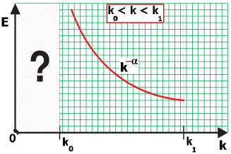
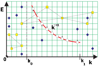
Figure 2.

In the last decade, this standard view proved to be incomplete while finite-size effects are well observable within inertial interval; this led first to introducing such special types of wave turbulence as frozen turbulence of capillary waves [48] and mesoscopic turbulence of gravity waves [65]. Quite recently, a novel two-layer model of laminated turbulence has been developed [27]. It allows to explain finite-size effects in the same frame: each small divisor leaves a gap in the power spectrum, shown as an empty circle in Fig.2 on the right. The lower boundary for the radius $\mathcal{R}$ of each circle can be computed using Thue-Siegel-Roth theorem [28] for the case of an irrational dispersion function, which covers all water waves (4)-(5). The gaps corresponding to the exact and quasi-resonances are shown by yellow squares; their dynamics is covered by the dynamical systems of corresponding resonance clusters ([24], Fig.1). Some gaps, shown by blue diamonds, correspond to the discrete modes that do not take part in resonances; they just keep their initial energies ([24], Fig.3).

Definition 4.1.

Solutions of (24) are called: exact resonances, if $\Omega=0;$ quasi-resonances, if

$$0<\mathcal{R}\leq\Omega\widetilde{<}(\partial\omega/\partial k)2\pi/L;$$

and approximate interactions, if

$$\Omega\gg(\partial\omega/\partial k)2\pi/L.$$

Exact resonances and quasi-resonances form discrete layer of turbulence, while approximate interactions form continuous layer. Correspondingly, the notion of discrete wave turbulence (DWT) is nowadays used, as opposed to CWT.

Remark 5.

Previous to our theory [27], the standard counterpart of CWT were low-dimensioned systems characterized by a small number of modes included. On the other hand, DWT is characterized by the clustering itself, and not by the number of modes in particular clusters which can be fairly big.

The minimal resonance broadening, necessary for quasi-resonances to appear, has been investigated numerically in [56] both for capillary and gravity water waves. Numerical simulations [54, 55, 56] showed that exact and quasi-resonances among the gravity waves are observable not on the time scale $\mathcal{O}(t/\varepsilon^{4})$ of kinetic theory but on the linear time scale. This means that dynamics of discrete layer but not the kinetic equation should be used as the base for a short-term forecast. The classical notion of wave interactions would be quite inappropriate – even misleading – for the description of all these important effects.

5. Summary

In 1981, in the paper with the title ”Wave interactions – evolution of the idea,” [47], O. Phillips wrote prophetical words: ”New physics, new mathematics and new intuition is required” in order to gain some understanding of finite-size effects in wave turbulent systems. Few years later, two – nowadays classical – books were published: ”Wave interactions and fluid flows,” [12], and ”Kolmogorov spectra of turbulence,”[66]. Appearing in 1985, the first one gives comprehensive account of the theory and experiments on exact resonances, quasi-resonances and approximate interactions – all together named wave interactions - of primary clusters in three- and four-wave systems. The second book came to world in 1992, with a beautiful statistical theory of wave turbulence which is due to the exclusion of exact resonances and quasi-resonances from the consideration. The first attempt to fill in the gap between these two treatises has been made in 1994, in a small paper ”Weakly nonlinear theory of finite-size effects in resonators”, [24]. Today, some 15 years later, we know much more about these effects and can formulate the three most important mathematical problems whose solutions would contribute enormously to our understanding of nonlinear resonance dynamics of water waves.

1st problem. Given a dispersion function and a small parameter, by some standard technique initial nonlinear PDE with fixed boundary conditions can be transformed into a set of dynamical systems corresponding to resonance clusters. Each of them is a Poincare normal form. Classification of all normal forms appearing this way according to their integrability properties is needed.

2nd problem. Wave turbulence with continuous spectra is described quite comfortably by the energy power spectra $k^{-\alpha}$, stationary solutions of kinetic equations: the only variable here is the wave length $k,$ while $\alpha$ is a parameter, defined by the wave type. Only the fact that the wave system has a conservation law, say its energy $E$, is used, not the value of $E.$ The finite answer is therefore independent on the initial conditions. The situation is different for discrete wave turbulence. Energy transfer is presently described by exact formulae (20) which are definitely not easy to use while initial values of the conservation laws (17) are included explicitly and they define the period of energy oscillation of each resonant mode. Some simplified description is needed, perhaps also stationary, with $\varphi$ regarded as a (different) constant at each moment of time.

3rd problem. To describe the transition from discrete to continuous layer of turbulence in terms of energy flow is a very challenging problem, which probably can not be solved before a simplified description of the discrete layer will be obtained.

Received xxxx 20xx; revised xxxx 20xx.

References

- [1] S. Annenkov and V. Shrira, Direct numerical simulations of downshift and inverse cascade for water wave turbulence, Phys. Rev. Lett., 96 (2006), 204501-1–204501-4.
- [2] A. Baker, “Transcendental Number Theory,” Cambridge University Press, 1975. (MR1074572)
- [3] T.B. Benjamin and J.E. Feir, The disintegration of wavetrains in deep water, Part 1, J. Fluid Mech., 27 (1967), 417–431.
- [4] M.D. Bustamante and E. Kartashova, Dynamics of nonlinear resonances in Hamiltonian systems, Europhys. Lett., 85 (2009), 14004-1–14004-5.
- [5] M.D. Bustamante and E. Kartashova, Effect of the dynamical phases on the nonlinear amplitudes’ evolution, Europhys. Lett., 85 (2009), 34002-1–34002-6.
- [6] M.D. Bustamante and E. Kartashova, Resonance clusters in the systems with cubic Hamiltonian. Part 1: Integrable dynamics, in preparation (2009)
- [7] C.C. Chow, D. Henderson and H. Segur, A generalized stability criterion for resonant triad interactions , J. Fluid Mech., 319 (1996), 67–76.(MR1406227)
- [8] A. Constantin and E. Kartashova, Effect of non-zero constant vorticity on the nonlinear resonances of capillary water waves, Europhys. Lett., 86 (2009), 29001-1–29001-6.
- [9] A. Constantin, D. Sattinger and W. Strauss, Variational formulations for steady water waves with vorticity, J. Fluid Mech., 548 (2006), 151–163. (MR2264220)
- [10] A. Constantin and W. Strauss, Exact steady periodic water waves with vorticity, Comm. Pure Appl. Math., 57 (2004), 481–527. (MR2027299)
- [11] A. Constantin and W. Strauss, Stability properties of steady water waves with vorticity, Comm. Pure Appl. Math., 60 (2007), 911–950. (MR2306225)
- [12] A.D. Craik, “Wave interactions and fluid flows,” Cambridge University Press, 1985. (MR0952373)
- [13] P. Denissenko, S. Lukaschuk and S. Nazarenko, Gravity surface wave turbulence in a laboratory flume, Phys. Rev. Lett., 99 (2007), 014501-1–014501-4.
- [14] A.I. Dyachenko, Y.V. Lvov and V.E. Zakharov, Five-wave interaction on the surface of deep fluid, Physica D, 87 (1995), 233–261.
- [15] E. Falcon, C. Laroche and S. Fauve, Observation of gravity-capillary wave turbulence, Phys. Rev. Lett., 98 (2007), 094503-1–094503-4.
- [16] G. Galileo, “Discorsi e dimostrazioni matematiche, intorno a‘ due nuove scienze,” Elsevier, Leiden, 1638.
- [17] I.G. Jonsson, Wave-current interactions, in “The Sea”, 65–120, Wiley, New York, 1990
- [18] J.L. Hammack and D.M. Henderson, Experiments on deep water waves with two-dimensional surface patterns, J. Offshore Mech. Artic Eng., 125 (2003), 48–53.
- [19] J.L. Hammack, D.M. Henderson and H. Segur, Progressive waves with persistent, two–dimensional surface patterns in deep water, J. Fluid Mech., 532 (2005), 1–51. (MR2262269)
- [20] K. Hasselmann, A criterion for nonlinear wave stability, J. Fluid Mech., 30 (1967), 737–739.
- [21] D. Hilbert, Mathematical problems, Bull. Amer. Math. Soc., 8 (1902), 437–479. (MR1557926)
- [22] D.M. Henderson, M.S. Patterson and H. Segur, On the laboratory generation of two–dimensional, progressive, surface waves of nearly permanent form on deep water, J. Fluid Mech., 559 (2006), 413–437.
- [23] E. Kartashova, Resonant interactions of the water waves with discrete spectra, in “Proceedings of Nonlinear Water Waves Workshop” (ed. D.H. Peregrine), pp. 43–53, University of Bristol, UK, 1992.
- [24] E. Kartashova, Weakly nonlinear theory of finite-size effects in resonators, Phys. Rev. Lett., 72 (1994), 2013–2016.
- [25] E. Kartashova, Wave resonances in systems with discrete spectra, in “Nonlinear Waves and Weak Turbulence” (ed. V.E. Zakharov), AMS Trans. 2, 95–129, 1998. (MR1618507)
- [26] E. Kartashova, Fast computation algorithm for discrete resonances among gravity waves, Low Temp. Phys., 145 (2006), 286–295.
- [27] E. Kartashova, A model of laminated turbulence, JETP Lett., 83 (2006), 341–345.
- [28] E. Kartashova, Exact and quasi-resonances in discrete water wave turbulence, Phys. Rev. Lett., 98 (2007), 214502-1–214502-4.
- [29] E. Kartashova and A. Kartashov, Laminated wave turbulence: generic algorithms I, Int. J. Mod. Phys. C, 17 (2006), 1579–1596. (MR2288656)
- [30] E. Kartashova and A. Kartashov, Laminated wave turbulence: generic algorithms II, Comm. Comp. Phys., 2 (2007), 783–794. (MR2337745)
- [31] E. Kartashova and A. Kartashov, Laminated wave turbulence: generic algorithms III, Physics A: Stat. Mech. Appl., 380 (2007), 66–74.
- [32] E. Kartashova and A. Kartashov, Exact and quasi-resonances among gravity-capillary waves, in preparation (2009).
- [33] E. Kartashova and V.S. L’vov, Cluster dynamics of planetary waves, Europhys. Lett., 83 (2008), 50012-1–50012-6.
- [34] E. Kartashova and G. Mayrhofer, Cluster formation in mesoscopic systems, Physics A: Stat. Mech. Appl., 385 (2007), 527–542.
- [35] E. Kartashova, S. Nazarenko and O. Rudenko, Resonant interactions of nonlinear water waves in a finite basin, Phys. Rev. E, 98 (2008), 0163041-1–0163041-9.
- [36] E. Kartashova, C. Raab, Ch. Feurer, G. Mayrhofer and W. Schreiner Symbolic computations for nonlinear wave resonances, in “Extreme Ocean Waves” (ed. E. Pelinovsky and Ch. Kharif), Springer, 97–128, 2008.
- [37] N. Kuznetsov, V. Maz’ya and B. Vainberg, “Linear water waves,” Cambridge University Press, 2002.
- [38] W. Lee, G. Kovacic and D. Cai. Renormalized resonance quartets in dispersive wave turbulence, Phys. Rev. Lett., 103 (2009), 024502-1–024502-4.
- [39] Y.V. Lvov, S. Nazarenko and B. Pokorni, Discreteness and its effect on water-wave turbulence, Physica D, 218 (2006), 24–35.
- [40] Yu. Matijasevich, The Diophantineness of Enumerable Sets, Soviet Math. Dokl, 11 (1970), 354–358.
- [41] L.F. McGoldrick, Resonant interactions among capillary-gravity waves, J. Fluid Mech., 21 (1967), 305–331.
- [42] J. Murdock, “Normal forms and unfoldings for local dynamical systems,” Springer-Verlag, New York, 2003. (MR1941477)
- [43] J. Pedlosky, “Geophysical fluid dynamics,” Springer-Verlag, New York, 1987.
- [44] O.M. Phillips, On the dynamics of unsteady gravity waves of infinite amplitude, J. Fluid Mech., 9 (1960), 193–217.
- [45] O.M. Phillips, Theoretical and experimental studies of gravity wave interactions, Proc. Roy. Soc. Lond., A299 (1967), 104–119.
- [46] O.M. Phillips, Wave interactions, in “Nonlinear waves” (eds. S. Leibovich and A.R. Seebass), 186–205, Cornell University Press, Ithaca and London, 1974.
- [47] O.M. Phillips, Wave interactions - evolution of an idea, J. Fluid Mech., 106 (1981), 215–227.
- [48] A.N. Pushkarev and V.E. Zakharov, Turbulence of capillary waves theory and numerical simulation, Physica D, 135 (2000), 98–116.
- [49] A.M. Rucklidge and M. Silber, Design of parametrically forced patterns and quasi-patterns, SIAM J. App. Dyn. Sys., 8 (1) (2009), 298–347.
- [50] H. Segur and D.M. Henderson, The modulation instability revisited, Euro. Phys. J. – Special Topics, 1147 (2007), 25–43.
- [51] H. Segur, D. Henderson, J. Hammack, C.-M. Li, D. Pheiff. and K. Socha., Stabilizing the Benjamin-Feir instability, J. Fluid Mechanics, 539 (2005), 25–4229–2713. (MR2262048)
- [52] L. Shemer and M. Stiassnie, Initial instability and long-time evolution of Stokes waves, in “The ocean surface” (eds. Y. Toba, H. Mitsuyasu and F.D. Reidel), 51–57, Dodrecht, Holland, 1985.
- [53] M. Stiassnie and L. Shemer, On the interactions of four water waves, Wave motion, 41 (2005), 307–328.
- [54] M. Tanaka, Verification of Hasselmann’s energy transfer among surface gravity waves by direct numerical simulations of primitive equations, J. Fluid Mech., 444 (2001), 199–221.
- [55] M. Tanaka, On the role of resonant interactions in the short-term evolution of deep-water ocean spectra, J. Phys. Oceanogr., 37 (2007), 1022–1036.
- [56] M. Tanaka and N. Yokoyama, Effects of discretization of the spectrum in water-wave turbulence, Fluid Dynamics Research, 34 (2004), 199–216.
- [57] F. Verheest, Proof of integrability for five-wave interactions in a case with unequal coupling constants, J. Phys. A: Math. Gen., 21 (1988), L545–L549. (MR0953204)
- [58] F. Verheest, Integrability of restricted multiple three-wave interactions. II. Coupling constants with ratios 1 and 2, J. Math. Phys., 29 (1988), 2197–2201. (MR0962556)
- [59] E. Wahlen, A Hamiltonian formulation of water waves with constant vorticity, Lett. Math. Phys., 79 (2007), 303–315. (MR2309783)
- [60] E. Wahlen, On rotational water waves with surface tension, Philos. Trans. R.Soc. Lon. Ser. A Math. Phys. Eng. Sci., 365 (1858) (2007), 2215–2225. (MR2329143)
- [61] G.B. Whitham, “Linear and nonlinear waves,” Wiley Series in Pure and Applied Mathematics, 1999. (MR1699025)
- [62] E.T. Whittaker, “A treatise on the analytical dynamics of particles and rigid bodies.,” Cambrige University Press, 1937. (MR0992404)
- [63] V.E. Zakharov, Statistical theory of gravity and capillary waves on the surface of a finite-depth fluid, Eur. J. Mech. B: Fluids, (1999), 327–344. (MR1701696)
- [64] V.E. Zakharov and N.N. Filonenko, Weak turbulence of capillary waves, J. Appl. Mech. Tech. Phys., 4 (1967), 500–515.
- [65] V.E. Zakharov, A.O. Korotkevich, A.N. Pushkarev and A.I. Dyachenko, Mesoscopic wave turbulence, JETP Lett., 82 (2005), 487–491.
- [66] V.E. Zakharov, V.S. L’vov and G. Falkovich, “Kolmogorov spectra of turbulence,” Series in Nonlinear Dynamics, Springer-Verlag, New York, 1992.
- [67] V.E. Zakharov and E.I. Shulman, Integrability of nonlinear systems and perturbation theory, in “What is integrability?” (ed. V.E. Zakharov), Springer, 185–250, 1990.