Collisionless plasma expansion in the presence of a dipole magnetic field

Abstract

The collisionless interaction of an expanding high–energy plasma cloud with a magnetized background plasma in the presence of a dipole magnetic field is examined in the framework of a 2D3V hybrid (kinetic ions and massless fluid electrons) model. The retardation of the plasma cloud and the dynamics of the perturbed electromagnetic fields and the background plasma are studied for high Alfvén–Mach numbers using the particle–in–cell method. It is shown that the plasma cloud expands excluding the ambient magnetic field and the background plasma to form a diamagnetic cavity which is accompanied by the generation of a collisionless shock wave. The energy exchange between the plasma cloud and the background plasma is also studied and qualitative agreement with the analytical model suggested previously is obtained.

I Introduction

When a high–energy density plasma is expanded into a magnetized background plasma, the injected plasma expands and excludes the background plasma and magnetic field to form a diamagnetic cavity. This process has been observed in a number of experiments in space and the laboratory (see, e.g., Ref. zak03 and references therein). The similar processes are responsible for the formation of the heliopause, where solar wind drags or convects magnetic fields from the Sun, which causes the deflection of both the interstellar medium and cosmic rays. Other examples of naturally occurring inflated or stretched magnetic fields include coronal mass ejections and the formation of the Earth’s magnetotail win05 ; win00 ; win98 . Starting in the 1960s, many experiments of the collisionless phenomena of exploding plasmas in space and laboratory were performed or planned. Dense, high–energy plasmas can also be formed by laser–irradiation of a small target embedded in a gas in an external magnetic field rip93 . The background gas can either be pre–ionized or be ionized by the laser. Such experiments show that, in addition to expansion, the target plasma is also subject to flute instabilities on its surface as it interacts with the background field and embedded plasma. The diamagnetic cavities are expected to occur also in supernova explosions dra02 . The physics of the plasma expansion and evolution has been investigated in detail numerically, using a variety of techniques, such as full particle win88 , hybrid (particle ions, fluid electron) bre87 and magnetohydrodynamics (MHD) hub92 codes. The properties of the expansion phase in the presence of either a stationary gis89 or a flowing background plasma win89 , as well as the details of unstable modes on the surface of the expanding plasma win89 ; hub90 ; bre92 , have been well studied.

Typical experimental parameters are such that the ions are collisionless but the situation for the electrons ranges from collisionless to collision–dominated. In this paper the dynamics of the expanding plasma cloud is studied for the completely collisionless regimes, which, in particular, are realized in many astrophysical processes (see, e.g., zak03 and references therein). An example is the problem of the collisionless retardation of the supernovae remnants which was first formulated by Oort oor46 and subsequently analyzed in detail by Shklovskii shk76 .

In recent years, the basic concept of the plasma expansion has been extended to consider a large magnetic bubble, which can be formed using a small magnetic coil and plasma source attached to a spacecraft, to efficiently inflate the bubble to a large cross–sectional area win00 ; win03 . A net force would be exerted on the spacecraft due to the deflection of the solar wind around the bubble. In this case, the plasma is continuously injected in the presence of a dipole or dipole–like magnetic field. Theoretical arguments par03 and calculations (see, e.g., Refs. win00 ; tan07 ; gar08 and references therein) suggest that the magnetic field of the dipole can be expanded with the plasma, so that the magnitude of the field falls off much slower with distance $r$ from the dipole, namely as $r^{-s}$, with $s\sim 1,2$ in certain directions at least, rather than $r^{-3}$ (for a bare dipole), allowing a large bubble to form. Laboratory experiments win01 ; win02 have provided some evidence for the slow falloff of the field from the source. However, the nature of the plasma and magnetic field expansion in this configuration is not completely understood, and how it compares with the more common picture of diamagnetic cavity formation has not been addressed to date. References zak03 ; win05 ; tan07 and the papers cited therein conducted a systematic study in a two–dimensional (2D) geometry and only for initial phase of expansion win05 , and in a three–dimensions (3D) but mainly of the characteristics of the magnetic field inflation tan07 . Special attention has been paid to the MHD analysis of the expanding plasma behavior in a dipole field in a vacuum mur01 , i.e. in the absence of the background plasma.

In this paper, in order to provide further insight into the underlying physics we have performed systematic particle–in–cell (PIC) 2D3V hybrid simulations of the plasma expansion in a magnetized background plasma in the presence of a dipole magnetic field. The basic parameters of the problem are introduced in Sec. II. The numerical method and model used are discussed in Sec. III. We perform a number of simulations assuming hydrogen cloud and hydrogen background plasmas and the results are presented and discussed in Sec. IV. Finally, we state the conclusions in Sec. V.

II Basic parameters for the plasma expansion

The plasma expansion process is characterized by the magnetic ($R_{m}$) and hydrodynamic ($R_{g}$) retardation lengths. $R_{m}$ is obtained by equating the initial kinetic energy $W_{0}$ of an initially spherical plasma cloud to the energy of the magnetic field that it pushes out in expanding to the radius $R_{m}$ rai63 , i.e., $R_{m}=(6W_{0}/H_{0}^{2})^{1/3}$. Here $H_{0}$ is the strength of the unperturbed magnetic field. As the plasma expands, it draws the background plasma into a combined motion. Along with this, the mass of expelled plasma increases. The radius of the sphere within which the mass of the plasma cloud and that of the background plasma drawn into the combined motion become equal is referred to as the hydrodynamic retardation length: $R_{g}=(3M/4\pi n_{b}m_{b})^{1/3}$, where $n_{b}$ and $m_{b}$ are the density and mass of the background plasma ions shk76 and $M$ is the mass of the expanding plasma. The smaller of the lengths, $R_{m}$ or $R_{g}$, determines the predominant mechanism for the retardation of the plasma cloud–magnetic or hydrodynamic. Of course $R_{m}$ and $R_{g}$ account for the ideal characteristics of the retardation process, therefore some high–energy particles may penetrate beyond the stopping length. The relation $R_{m}/R_{g}\sim M_{A}^{2/3}$, where $M_{A}=u/v_{A}$ is the Alfvén–Mach number ($u\sim(W_{0}/M)^{1/2}$ is the initial expansion velocity of the plasma) and $v_{A}=H_{0}/\sqrt{4\pi n_{b}m_{b}}$ is the Alfvén velocity in the background plasma, implies that for $M_{A}\ll 1$ the cloud loses energy as a result of the deformation and displacement of the magnetic field, while for $M_{A}\gg 1$ the retardation is caused by the interaction with the background plasma zak88 ; osi03 (see also Ref. zak03 ). In this paper we consider only the second (hydrodynamic) regime of collisionless expansion with $M_{A}\gg 1$. In this case the retardation length is given by $\ell_{s}\simeq R_{g}$.

An analysis shows that the hydrodynamic retardation can only be ensured by a collisionless laminar (or turbulent) mechanism zak88 associated with the generation of vortical electric fields $E_{i}$ in the front of the expanding plasma or by a collisional mechanism owing to pairwise collisions of the cloud ions with the ions and electrons of the background plasma. The ions of the expanding plasma transfer their energy to the ions and electrons of the background plasma in multiple ion–ion or ion–electron Coulomb collisions with a mean free paths $\lambda_{ii}$ and $\lambda_{ei}\sim(m_{e}/m_{c})\lambda_{ii}$, respectively tru65 ; koo72 . Here $m_{e}$ and $m_{c}$ are the electron and cloud ion masses, respectively. In this paper we assume a completely collisionless regimes when $\lambda_{ii}\gg\lambda_{ei}>\ell_{s}$. Strictly speaking, the hydrodynamic description is inapplicable under these conditions. However, as shown in Ref. rai95 the hydrodynamic approach, when considering collisionless plasma expansion into the magnetized, ionized medium, can give quite reasonable qualitative and even satisfactory quantitative results. The physical reason underlying this situation is the small ion cyclotron radius $a_{L}$ in comparison with a characteristic flow scale $\ell_{s}$, with the ion cyclotron radius playing the role of particle mean free path.

The first group of the collisionless interaction mechanisms are collective turbulent mechanisms (anomalous viscosity, anomalous resistivity) during the development of ion–ion or electron–ion beam instabilities win84 . The condition for excitation of the ion–ion instability has the form $u^{2}\leqslant v_{A}^{2}+2c_{s}^{2}$ (see, e.g., Ref. pap71 ) or $M_{A}^{2}\leqslant 1+2c_{s}^{2}/v_{A}^{2}$, where $c_{s}=\sqrt{T_{e}/m_{b}}$ is the ion sound speed in the background plasma. In many typical situations $v_{A}\gtrsim c_{s}$ and $M_{A}\lesssim 2$. Thus, according to the criteria mentioned above at high Alfvén–Mach numbers $M_{A}\gg 1$ the retardation of the expanding plasma cannot be caused by the turbulent mechanisms.

The second group is the collisionless laminar retardation mechanism associated with the generation of vortical electric fields. It is known that the role of vortical electric fields becomes predominant as $M_{A}$ increases, since $E_{i}/E_{p}\sim M_{A}^{2}$ zak88 , where $E_{p}$ is the polarization electric field which arises as a result of the drop of the hydrodynamic and magnetic pressures at the front of the plasma cloud. A model for energy exchange between the cloud and the background plasma due to the combined effect of the gyromotion of the ions and the generation of vortical electric fields when $M_{A}>1$ (so–called magnetolaminar mechanism (MLM)) has been proposed in Ref. gol78 . Analytic solutions for the initial expansion phase, when only a vortical electric field $E_{i}$ develops, showed that the fraction of energy transferred from the cloud to the background plasma is proportional to $\delta=(R_{g}/a_{L})^{2}$ (MLM interaction parameter), where $a_{L}$ is the cyclotron radius of the cloud ions.

In the framework of the ideal MHD approximation for the description of the plasma expansion into a vacuum in the presence of dipole magnetic field, another energetic parameter $\kappa$ was defined which is given by $\kappa=W_{0}/W_{M}$ nik93 , where $W_{M}$ is the total magnetic energy of the dipole beyond the spherical radius $r_{d}$ ($W_{M}=p^{2}/3r_{d}^{3}$), $r_{d}$ is the distance from the dipole to the center of the plasma cloud and $p$ is the magnetic moment magnitude. Nikitin et al. introduced critical value $\kappa_{c}$ for a different plasma location nik93 . In the case when $\kappa<\kappa_{c}$, a substantial plasma retardation will occur in all directions from the cloud center location (”quasi–capture” mode), meanwhile the plasma will not be captured by an ambient magnetic field when $\kappa>\kappa_{c}$ (”rupture” mode). The critical value varies between $0.1$ and $0.4$. The latter value is realized when the plasma cloud is located at the dipole axis. In this paper we consider only the second regime of the plasma expansion.

III Collisionless hybrid simulation

The hybrid model is used to study the collisionless plasma expansion in a magnetic field. This model describes the ions by means of the velocity distribution function $f(\mathbf{r},\mathbf{v},t)$, the electrons being considered hydrodynamically hae81 ; ler84 . The typical scale on which the macroscopic parameters (the plasma density, magnetic field) vary is the ion cyclotron radius $a_{L}$. The electron cyclotron radius $a_{Le}$ is much less than $a_{L}$ due to the small electron mass. Of course, the electron distribution function changes sharply on a small scale $a_{Le}$, but we do not consider such details. If we are interested in the behavior of those macroscopic parameters that vary on a scale $a_{L}$, it is sufficient to consider only the motion of the electron small–scale gyromotion centers. In this case one can consider the electrons as a fluid and describe their motions hydrodynamically.

All of the estimates show that the plasma under the conditions in question is essentially quasineutral everywhere, although there are thin space charge regions. These regions are located near the plasma cloud boundary as well as near the collisionless shock in the background plasma. The scales of these regions are essentially less than $a_{L}$, and therefore, they are not considered here. Then the densities of ions $n_{\alpha}$ and electrons $n_{e}$ in quasineutral plasma satisfy the condition $n_{e}=\sum_{\alpha}Z_{\alpha}n_{\alpha}$, where $Z_{\alpha}e$ is the charge of the ion from plasma species $\alpha$. Let the cloud ions have the index $\alpha=c$, whereas the index of the background ions is $\alpha=b$. The ion distribution functions $f_{\alpha}$ are governed by the Vlasov kinetic equation

$$\frac{\partial f_{\alpha}}{\partial t}+{\mathbf{v}}\cdot\frac{\partial f_{\alpha}}{\partial{\mathbf{r}}}+\frac{Z_{\alpha}e}{m_{\alpha}}\left({\mathbf{E}}+\frac{1}{c}\left[{\mathbf{v}}\times{\mathbf{H}}\right]\right)\cdot\frac{\partial f_{\alpha}}{\partial{\mathbf{v}}}=0.$$ (1)

The electric and magnetic fields satisfy the Maxwell equations

$$\boldsymbol{\nabla}\times{\mathbf{H}}=\frac{4\pi n_{e}e}{c}\left(\mathbf{v}_{i}-\mathbf{v}_{e}\right),\quad\boldsymbol{\nabla}\times\mathbf{E}=-\frac{1}{c}\frac{\partial\mathbf{H}}{\partial t}$$ (2)

in which the displacement current is omitted. We assume non–relativistic expansion velocity of the plasma cloud. Here $\mathbf{v}_{i}$ is the ion mean velocity which is defined as

$$n_{e}=\sum_{\alpha}Z_{\alpha}n_{\alpha},\quad\mathbf{v}_{i}=\frac{1}{n_{e}}\sum_{\alpha}Z_{\alpha}n_{\alpha}\mathbf{v}_{\alpha},$$ (3)

$$n_{\alpha}=\int f_{\alpha}d\mathbf{v},\quad\mathbf{v}_{\alpha}=\frac{1}{n_{\alpha}}\int\mathbf{v}f_{\alpha}d\mathbf{v}.$$ (4)

The mean electron velocity $\mathbf{v}_{e}$ satisfies the equation

$$\mathbf{E}=-\frac{1}{c}\left[\mathbf{v}_{e}\times\mathbf{H}\right]$$ (5)

which can be derived from the hydrodynamic equation of motion of electrons ignoring the inertial term (i.e. formally by taking the limit $m_{e}\to 0$). The electric field in Eq. (5) is that required to keep the electrons and ions together ensuring the quasineutrality of the plasma. Thus, we do not resolve the expansion process on the Debye scale. One can interpret Eq. (5) as follows. The electromagnetic force acting on the electrons and ions does not depend on the particle mass; therefore light electrons are accelerated much more than ions. This would lead to charge separation and would violate the quasineutrality condition if the strong Coulomb interaction would not prevent this from occurring; i.e., an appropriate electric field arises to enforce quasineutrality. The mean force itself, which so strongly accelerates the electron gas, has to disappear or, more exactly, its electric component has to compensate the Lorentz force within the accuracy of the order of $m_{e}/m_{\alpha}$. This fact is expressed by the approximate relation (5). Equations (1)–(5) constitute a closed system and are used to investigate the collisionless plasma dynamics in an external magnetic field.

Note that in Eqs. (1)–(5) we have also neglected the terms associated with the finite conductivity (e.g. magnetic field diffusion and Joule heating). It can be shown that this approximation is easily satisfied in a wide range of parameters. In fact, for example, we can estimate the characteristic diffusion time for the magnetic field, $\tau_{m}=4\pi a_{L}^{2}\sigma/c^{2}$, where $\sigma$ is the conductivity of the plasma. Introducing the characteristic retardation time of the plasma cloud $\tau_{s}=R_{g}/u$ we obtain $\tau_{m}/\tau_{s}\sim M_{A}^{2}(\lambda_{ii}/R_{g})\gg 1$. Here $\lambda_{ii}$ is the mean free path for ion–ion Coulomb interaction.

These approximations constitute the hybrid collisionless plasma model employed in this paper. It should be emphasized that earlier simulations and experiments demonstrated the practical realizability of the magnetolaminar interaction model zak03 ; zak88 discussed briefly in Sec. II. In addition it can be shown that Eqs. (1)–(5) of the hybrid model have universal nature. This universality can be demonstrated by normalizing Eqs. (1)–(5) and all the quantities with the scales $n_{b0}$ (densities), $c/\omega_{pb}$ (lengths), $v_{A}$ (velocities) $H_{0}$ (magnetic field), $(v_{A}/c)H_{0}$ (electric field). In these units the time and the ionic distribution functions are scaled by the cyclotron period $\Omega^{-1}_{b}$ and $n_{b0}/v^{3}_{A}$, respectively. Here $\omega_{pb}$, $\Omega_{b}$ and $n_{b0}$ are the plasma and cyclotron frequencies and the unperturbed (initial) density of the background ions, respectively. $v_{A}$ is the Alfvén velocity in the background plasma. Then it is seen that Eqs. (1)–(5) depend only on the dimensionless parameters $Z_{c}/Z_{b}$ and $Z_{c}m_{b}/Z_{b}m_{c}$.

Figure 1: Scheme of the simulation region showing location of the dipole and the initial position of the plasma cloud.

Let us consider axially symmetric model for the dynamics of a point explosion that forms a cloud of dense plasma expanding into a magnetized low–density background plasma. For a simplicity we assume hydrogen cloud and background plasmas with $m_{c}=m_{b}=m_{p}$, $Z_{c}=Z_{b}=1$, where $m_{p}$ is the proton mass. At the initial time $t=0$, an explosion occurs at the point $\rho=z=0$ in a cylindrical region $0\leqslant\rho\leqslant L_{\rho}$, $-L_{z}\leqslant z\leqslant L_{z}$ (see Fig. 1) filled with a homogeneous background plasma of density $n_{b0}$. The magnetic dipole with a moment $\mathbf{p}=p_{z}\mathbf{e}_{z}$ creates a magnetic field $\mathbf{H}_{0}(\mathbf{r})=\mathbf{H}_{0}(\boldsymbol{\rho},z)$ and is placed outside the cylindrical region on the $z$–axis ($z_{d}<-L_{z}$, $\boldsymbol{\rho}_{d}=0$). Here $\rho,z,\varphi$ are the cylindrical coordinates and $\boldsymbol{\rho}$ is the cylindrical radius vector. Similarly $r,\theta,\varphi$ are the spherical coordinates with the radius vector $\mathbf{r}$, and $\theta$ is the angle between $\mathbf{r}$ and the $z$–axis. We consider the case when the dipole moment is parallel to the $z$–axis and due to the symmetry we chose $p_{z}>0$. In our simulations the dipole magnetic field is determined by the ratio $\eta=H_{0}(0,-L_{z})/H_{0}(0,L_{z})>1$ and the strength of the dipole magnetic field at the center of the simulation domain, i.e. $H_{0}=H_{0z}(0)>0$. Using these two quantities it is easy to obtain the position $z_{d}$ and the moment $p_{z}$ of the dipole

$$p_{z}=-\frac{z_{d}^{3}}{2}H_{0},\qquad z_{d}=-L_{z}\frac{\eta^{1/3}+1}{\eta^{1/3}-1}$$ (6)

which completely determine the dipole field for given length $L_{z}$. At fixed $H_{0}$ the limits $\eta\to 1$ and $\eta\gg 1$ correspond to nearly homogeneous and strongly inhomogeneous dipole magnetic fields in a cylindrical region, respectively. Throughout this paper the cyclotron frequency $\Omega_{b}$ and the Alfvén velocity $v_{A}$ are determined in terms of the magnetic field $H_{0}$. Note that due to the axial symmetry all physical quantities are independent on the azimuthal angle $\varphi$ (obviously this symmetry breaks down for arbitrary orientation of the magnetic moment $\mathbf{p}$). Here we neglect the $\varphi$–derivatives in Eqs. (1)-(5) and consider 2D3V model for our simulations. It should be also emphasized that the scheme outlined in Fig. 1 essentially differs from one adopted in Refs. win05 ; tan07 where the dipole is located inside the simulation domain and due to the strong interactions the ions may be trapped by the dipole.

The explosion forms a cloud of dense plasma of radius $r_{0}$ containing $N_{c}$ ions with a total kinetic energy $W_{0}$. At the initial time, the velocity of the cloud ions is distributed linearly along the radius, i.e. at $r\leqslant r_{0}$

$$v_{r}\left(r,0\right)=u(r)=v_{m}\frac{r}{r_{0}}$$ (7)

and $v_{r}(r,0)=0$ at $r>r_{0}$. Here $v_{m}$ is the maximal velocity of the ions in the cloud and is determined by the initial energy $W_{0}$ of the cloud, with $v_{m}=(10W_{0}/3N_{c}m_{p})^{1/2}=v_{0}(5/3)^{1/2}$, where $v_{0}=(2W_{0}/N_{c}m_{p})^{1/2}$ is the average velocity of the cloud ions.

The equation of the energy conservation of the system is given by

$$W=W_{\mathrm{kin}}+2\pi\int_{0}^{L_{\rho}}\rho d\rho\int_{-L_{z}}^{L_{z}}dz\left(\frac{1}{2}nmv_{e}^{2}+\frac{H^{2}}{8\pi}\right).$$ (8)

Here $n=n_{e}$, and $n$ is the total density of the ions in the cloud and background plasmas. The total energy of the system consists of the kinetic energies of the electron gas, the energy of the magnetic field, and the kinetic energy $W_{\mathrm{kin}}$ of the ions. Note that in Eq. (8) we have neglected the energy of the electric field as $v_{e}\ll c$ and $E\ll H$.

The system size employed in the computations is $2L_{z}=9.8a_{L}$ and $L_{\rho}=4.9a_{L}$ and uses $98\times 49$ cells in $z$ and $\rho$ directions, respectively, where $a_{L}=v_{m}/\Omega_{b}$ is the ion cyclotron radius. Thus, the cell size in the $\rho$ and $z$ directions is $h=h_{\rho}=h_{z}=0.1a_{L}$. In order to correctly resolve the ion gyromotion the quantity $h$ and the time step $\Delta t$ are fraction of the ion cyclotron radius $a_{L}$ and the ion cyclotron period $\Omega^{-1}_{b}$, respectively. In our simulations $\Delta t=0.01\Omega^{-1}_{b}$. The initial radius $r_{0}$ of the plasma cloud is considerably smaller than the step size $h$; that is, we can assume that at the initial time the cloud is concentrated at a point. At the initial time $t=0$ we take the background plasma at rest and assume that the background particles are distributed uniformly over the entire cylindrical region and the particles of the expanding plasma are distributed uniformly in the cloud. Explicitly the initial distribution functions of the background and cloud ions are given by $f_{b}(\mathbf{r},\mathbf{v},0)=n_{b0}\delta(\mathbf{v})$ and $f_{c}(\mathbf{r},\mathbf{v},0)=n_{c0}\delta(\mathbf{v}-u(r)\frac{\mathbf{r}}{r})$, respectively, where $n_{c0}$ is the initial density of the cloud ions and $u(r)$ is determined by Eq. (7). Note that the distribution function $f_{c}(\mathbf{r},\mathbf{v},0)$ is non–zero only at $0\leqslant r\leqslant r_{0}$. Boundary conditions are one of the most important conditions to be satisfied in an electromagnetic problem, and they vary depending on the problem. In Ref. win05 , periodic boundary conditions are imposed on the fields and the particles. They only run the system a relatively short amount of time before any disturbances reach the edges of the system. In this paper, at the boundaries of the cylindrical region $\rho=L_{\rho}$ and $z=\pm L_{z}$, all quantities are specified by its unperturbed values, and on the $z$–axis (i.e. at $\rho=0$) we assume the condition $E_{\rho,\varphi}=H_{\rho,\varphi}=v_{e\rho,\varphi}=0$ which is a natural consequence of the symmetry of the model. The absorption boundary conditions are chosen for all the particles which means that any particle leaving the computation domain is assumed to have gotten lost. With these boundary conditions the calculations are continued until the time the perturbations reach the boundaries of the cylindrical region.

Table 1: The values of the parameters for the numerical simulation ($M_{A}=15$, $\delta=1$). The number of the ions (protons) in a cloud is $N_{c}=1.67\times 10^{19}$.

$a_{L}=34.16$ cm	$R_{g}=34.16$ cm	$R_{m}=175.2$ cm	$\tau_{s}=1.044$ $\mu$s
$H_{0}=100$ G	$W_{0}=0.896$ kJ	$v_{m}=3.27\times 10^{7}$ cm/s	$\eta=100$
$n_{b0}=10^{14}$ cm-3	$v_{A}=2.18\times 10^{6}$ cm/s	$\Omega_{b}=9.58\times 10^{5}$ s-1	$\omega_{pb}=1.32\times 10^{10}$ s-1

The equations of motion for the ions are the equations of the characteristics of the Vlasov kinetic equation (1). Assuming hydrogen plasma we obtain

$$\dot{\mathbf{r}}_{i}={\mathbf{v}}_{i},\qquad\dot{\mathbf{v}}_{i}=\frac{e}{m_{p}}\left({\mathbf{E}}+\frac{1}{c}\left[{\mathbf{v}}_{i}\times{\mathbf{H}}\right]\right).$$ (9)

These equations are solved by the particle-in-cell (PIC) method using Boris pusher algorithm hoc88 ; bir04 . Instead of the kinetic equation integration, the trajectories of a large number of the quasi–particles (each of these particles in turn consist of the large number of ions) are computed. In our simulations the total number of the quasi–particles is $97000$ and $20168$ quasi–particles are used for a cloud. For the background plasma we set $16$ quasi–particles in the cell with close values of the cyclotron radii (because $h\ll a_{L}$) which allows us to simulate ion kinetics in details. Further increasing the number of the quasi–particles does not essentially influence the simulation results. The Maxwell equations are solved using an explicit first order splitting scheme on staggered grid. A more detailed description of the mathematical model and the numerical simulation can be found, for example, in Refs. ler84 ; hoc88 ; bir04 .

IV Results

In this section, results from several calculations are presented to describe the overall physics and to show the properties of the resulting structures. Numerical simulations have been performed for calculation of the energy, density and electromagnetic characteristics of the expansion of a hydrogen plasma into a uniform magnetized background hydrogen plasma at high Alfvén–Mach numbers with $M_{A}=v_{m}/v_{A}=15.0$ and for a MLM interaction parameter $\delta=1.0$. The basic physical parameters of the simulations are shown in Table 1, where $\tau_{s}=R_{g}/v_{m}$ is the hydrodynamic retardation time. Note that $R_{g}\ll R_{m}$ and the retardation of the cloud is caused here by the interaction with the background plasma. The dipole is placed at $z_{d}=-258.86$ cm (see Fig. 1). The initial radius of the plasma cloud is $r_{0}=0.01a_{L}$ which corresponds to the initial density $n_{c0}=10^{20}$ cm^-3. The parameter $\kappa$ introduced in Sec. II is $\kappa=0.62>\kappa_{c}$. Thus we expect that the ions will not be captured by a dipole magnetic field. Using the parameters introduced above, the simulation is run to $t\simeq 5\tau_{s}$ when the perturbation reach to the boundaries of the cylindrical region and the boundary conditions adopted here become invalid. Due to the cylindrical symmetry the solutions of Eqs. (1)–(5) are obtained using the cylindrical coordinate system shown in Fig. 1.

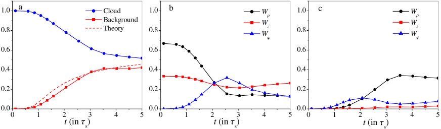
Figure 2: (Color online) The time (in units of $\tau_{s}$) variation of the kinetic energy (in units of $W_{0}$) of the plasma cloud and background plasma particles for $M_{A}=15.0$, $\delta=1.0$. a) The variation of the total energy of the background plasma (squares) and plasma cloud (circles). The dashed line is the theoretical predictions of Ref. gol78 (see the text for details). b) The time variation of the radial ($W_{\rho}$, circles), longitudinal ($W_{z}$, squares) and rotational ($W_{\varphi}$, triangles) energies of the plasma cloud. c) The same as in b) but for background plasma.

Figure 2 shows the time variation of the kinetic energies of the cloud and the background plasma. The energies are normalized to the initial energy of the plasma cloud $W_{0}$ and the time is given in units of the retardation time $\tau_{s}$. It is seen that the energy of the plasma cloud decreases with a time and at $t\simeq 5\tau_{s}$, about a half of the initial energy is transferred to the background plasma. Let us recall that the Coulomb collisions between particles are completely ignored here and thus as mentioned in Sec. II the energy transfer is caused by the MLM interaction. In Ref. gol78 a simple analytical model was suggested for the energy transfer from the plasma cloud to the ambient plasma in the presence of a homogeneous magnetic field. Assuming the initial distribution functions $f_{c}(\mathbf{r},\mathbf{v},0)=N_{c}\delta(\mathbf{r})f_{0}(v)$ and $f_{b}(\mathbf{r},\mathbf{v},0)=n_{b}\delta(\mathbf{v})$ of the ions in the plasma cloud and the background plasma, respectively, the energy transfer in this model reads (see Ref. gol78 for details)

$$\frac{\Delta W(t)}{W_{0}}=\frac{\delta}{6}\left[\kappa^{5}(t)+5\int_{\kappa(t)}^{\infty}\chi^{2}\left(x,t\right)dx\right],$$ (10)

where

$$\varphi\left(u\right)=4\pi\int_{u}^{\infty}f_{0}(v)v^{2}dv,\quad\chi\left(x,t\right)=x^{2}-\left[x^{3}-\varphi\left(\frac{R_{g}x}{t}\right)\right]^{2/3}.$$ (11)

Here the velocity distribution function $f_{0}(v)$ is normalized according to $\varphi(0)=1$ and the quantity $\kappa(t)$ is determined from the equation

$$\kappa^{3}(t)=\varphi\left(\frac{R_{g}\kappa(t)}{t}\right).$$ (12)

Assuming that the strength of the homogeneous magnetic field is $H_{0}$ and the velocity distribution function $f_{0}(v)=(3/4\pi v^{3}_{m})H(v_{m}-v)$ (where $H(z)$ is the Heaviside unit–step function) the prediction of this model is shown in Fig. 2a (the dashed line). The transferred energy (10) at $t<\tau_{s}$ and for a chosen $f_{0}(v)$ is then given by $\Delta W(t)/W_{0}\simeq(\delta/6)(t/\tau_{s})^{5}$ and in the limit $t\to\infty$ approaches $\Delta W_{\infty}/W_{0}=C\delta$ (where $C\simeq 0.59$) independently of the particles initial velocity distribution function in a cloud. It is seen that the theory agrees qualitatively with the simulation (squares) although it has been derived under assumption that $\Delta W(t)\ll W_{0}$. The sum of the cloud and background plasma energies is the total kinetic energy $W_{\mathrm{kin}}(t)$ of the ions involved in the energy conservation relation, Eq. (8). This energy decreases with a time due to the energy transfer to the electrons (second term in Eq. (8)) and the magnetic field (last term in Eq. (8)). However the amount of the energy gained by the electrons and the magnetic field is small compared to $W_{\mathrm{kin}}$.

The time variation of the radial ($W_{\rho}$), longitudinal ($W_{z}$) and gyromotion ($W_{\varphi}$) components of the energies are shown in Fig. 2b,c. Using Eq. (7) it is easy to calculate the radial and longitudinal energies of the plasma cloud at $t=0$ which are given by $W_{\rho}(0)=(2/3)W_{0}$ and $W_{z}(0)=(1/3)W_{0}$, respectively. At the initial time there is no gyromotion of the particles and $W_{\varphi}(0)=0$. As shown in Fig. 2b,c the expanding plasma cloud loses its radial energy which is transferred to the gyromotion energy of the cloud and the background plasma ions. In addition a large amount of the cloud kinetic energy is transferred to the radial energy of the background ions. It is also seen that the changes of the longitudinal energies of the ions are small.

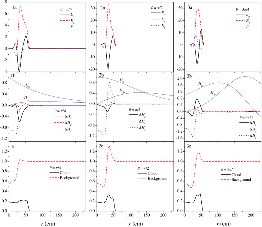
Figure 3: (Color online) The perturbations of the electromagnetic fields and the densities of the plasma cloud and background plasma as functions of the spherical coordinate $r$ (in cm) for $t=2\tau_{s}$, $M_{A}=15.0$ and $\delta=1.0$ and for some values of $\theta$. The panels 1a–3a show the distributions of the $\rho$ (solid lines), $\varphi$ (dashed lines), and $z$ (dotted lines) components of the electric field (in units of $(v_{A}/c)H_{0}$) at $\theta=\pi/4$, $\theta=\pi/2$ and $\theta=3\pi/4$, respectively. The panels 1b–3b show the same as 1a–3a but for the perturbation of the magnetic field $\Delta\mathbf{H}$ (in units of $H_{0}$). The components of the dipole magnetic field $H_{0z}$ and $H_{0\rho}$ are also shown as thin solid lines. 1c–3c show the densities (in units of $n_{b0}$) of the cloud (solid lines) and the background plasma (dashed lines) at $\theta=\pi/4$, $\theta=\pi/2$ and $\theta=3\pi/4$, respectively.

Figure 3 shows the electric (panels 1a–3a) and the perturbed magnetic ($\Delta\mathbf{H}(\mathbf{r},t)=\mathbf{H}(\mathbf{r},t)-\mathbf{H}_{0}(\mathbf{r})$, panels 1b–3b) fields strengths in units of $(v_{A}/c)H_{0}$ and $H_{0}$, respectively, as well as the densities (panels 1c–3c) of the cloud and the background plasma in units of $n_{b0}$ as the functions of $r$ (in cm) at $t=2\tau_{s}$, $\theta=\pi/4$, $\theta=\pi/2$ and $\theta=3\pi/4$. Here $\theta$ is the angle between the spherical radius vector $\mathbf{r}$ and the $z$–axis. In the panels 1b–3b of Fig. 3 the radial $H_{0\rho}$ and longitudinal $H_{0z}$ components of the dipole magnetic field are also shown (note that $H_{0\varphi}=0$) as thin solid lines. As expected the density of the plasma cloud is strongly reduced due to the expansion. In addition the perturbations of the electromagnetic fields are larger at $\theta\geqslant\pi/2$ where the dipole magnetic field is stronger. At the initial stage of the expansion process ($t\ll\tau_{s}$) the ions of the plasma cloud front propagates through a quiescent background plasma, and different plasmas are mixed. At this stage the background ions are accelerated mainly by the generated azimuthal electric field. Then, turning under the Lorentz force action, they acquire the radial velocity. At the later stage when the radial and longitudinal electric fields arise, the motionless background ions acquire a velocity due to all components of the field, with the azimuthal and radial fields being dominant. In general the motion of the ions in the electric and magnetic fields is very complicated. They will do a gyromotion along the magnetic field lines. But along with the gyromotion, the ions will also experience $\mathbf{E}\times\mathbf{H}$ drift and gradient drift. In contrast to the azimuthal electric field, the radial and longitudinal components of $\mathbf{E}$ are space–charge fields. This follows from Eq. (5) as the electromagnetic induction Eq. (2) provides the azimuthal field generation rather than the radial and longitudinal ones. The electric field is generated in a region of the perturbation of the magnetic field, and everywhere it is perpendicular to the total field $\mathbf{H}$.

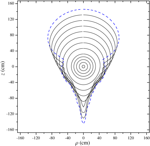
Figure 4: (Color online) The evolution of the boundary of the plasma cloud from $t=0.11\tau_{s}$ (central circle) to $t\simeq 5\tau_{s}$ (external dashed line). The time interval between two successive lines is approximately $\Delta t\simeq 0.4\tau_{s}$.

From Fig. 3 it is seen that the retardation of the plasma cloud is accompanied by the formation of a compressed plasma layer which moves together with the compressed electromagnetic field; i.e., a collisionless shock wave is formed. The depth of the compressed layer is of the order of the ion cyclotron radius $a_{L}$, in agreement with an estimate $\Delta\sim a_{L}$ of the width $\Delta$ of the collisionless shock front given in Ref. sag66 . The ions of the background plasma are pushed out of the expansion region; this leads to the formation of a plasma cavity. It correlates with the diamagnetic cavity, a region in which the total magnetic field $\mathbf{H}(\mathbf{r},t)$ is smaller than the unperturbed dipole field because it is squeezed out (Fig. 3). Thus, there is essentially no electric field in the cavity. Due to the retardation of the ions of the plasma cloud front, a part of its mass forms a shell near the front boundary, see panels 1c–3c of Fig. 3. However this shell is not isotropic and is more visible at $\theta\geqslant\pi/2$, i.e. in the region closer to the dipole. At the later time of the expansion $t>2\tau_{s}$ the plasma shell becomes more and more pronounced with the formation of the cavity also in the plasma cloud with sharply (with the width $\sim a_{L}$) distributed ions.

The time evolution of the plasma cloud boundary is shown in Fig. 4, where the central circle and external dashed lines correspond to $t=0.11\tau_{s}$ and $t\simeq 5\tau_{s}$, respectively. As shown in Fig. 4 an initially symmetrical plasma cloud begins to be asymmetric in the $\rho z$ plane at $t\gtrsim 2\tau_{s}$. On the other hand the shape of the cloud is symmetrical at all the stages in the plane perpendicular to the $z$–axis (not shown). The similar shape of the plasma cloud is observed in the experiments as well as in numerical simulations of the plasma expansion in a vacuum when the background plasma is absent zak03 ; mur01 . In this case the asymmetrical pattern may be caused only by the ambient magnetic field. At the initial stage, the plasma cloud expands isotropically as a free stream with high kinetic energy. Then, plasma expanding downward begins to decelerate because the ambient dipole magnetic field is stronger at a lower region near the dipole (see, e.g., Figs. 1 and 4). The kinetic beta $\beta_{c}$ defined as the ratio of plasma cloud kinetic energy density to magnetic energy density reaches unity around this area first, and then strong interaction between plasma and the ambient field occurs. Thus, the diamagnetic motion of plasma is induced to generate the surface diamagnetic current asymmetrically, only on the lower plasma surface. In Ref. ner06 an analytical model was suggested to calculate the pressure of the dipole magnetic field on the surface of the plasma cloud. It was shown that at $\mathbf{p}=p_{z}\mathbf{e}_{z}$ this pressure vanishes at $\theta=0;\pi$ and has its maximum at $\theta=\theta_{\max}$ ($\pi/2<\theta_{\max}<\pi$) which depends on the ratio $R/|z_{d}|$. Here $R$ is the radius of the plasma cloud. The maximal value $\theta_{\max}$ tends to $\pi$ with increasing $R$ and shifts towards the value $\theta_{\max}\simeq\pi/2$, when $R\to 0$. Therefore the layer near $\theta\simeq\theta_{\max}$ of the expanding plasma sphere will be mainly deformed by the external magnetic pressure. In the present context of the high–energy expansion $\beta_{c}\gg 1$ even at the later stages of the expansion and the magnetic field cannot deform directly the cloud shape. In this case the deformation occurs due to the interaction with the background plasma with initially low kinetic $\beta_{b}$. Then the background plasma tends to change the shape to follow the dipole magnetic field lines. As shown in Fig. 2 the kinetic energy of the background ions and hence the parameter $\beta_{b}$ increases with time which leads to the formation of the asymmetrical kinetic pressure of the background ions on the plasma cloud.

V Conclusions

In this paper we have investigated the collisionless expansion of the dense plasma cloud into magnetized background plasma in the presence of a dipole magnetic field. The 2D3V hybrid–PIC simulations with kinetic ions and massless fluid electrons have been employed. We have considered the case of high–energy super–Alfvénic expansion with $M_{A}\gg 1$ when the expanding plasma is not captured by the ambient magnetic field. It is shown that in this parameter regime the retardation and the deformation of the plasma cloud is mainly caused by the interaction with background plasma which, however, can be strongly affected (at least at the initial stage) by a magnetic field. Our numerical results for the energy transfer from the plasma cloud to the background plasma have been compared with the theoretical predictions of Ref. gol78 and qualitatively good agreement has been found. For future applications the arbitrary orientation of the dipole (with respect to the $z$–axis, see Fig. 1) should be considered. For instance, such a configuration has been realized in the experiment mur01 . In this case the physical quantities also depend on the azimuthal angle $\varphi$ and the shape of the plasma cloud becomes asymmetric in the plane perpendicular to the $z$–axis.

An additional item for further investigations is the development of a model which accounts the thermal effects for electrons which are completely neglected in the current study. These effects can be included by adding in the right hand side of Eq. (5) the term $-(1/en)\boldsymbol{\nabla}p_{e}$, where $p_{e}$ is the thermal pressure of the electrons. Also along with Eqs. (1)–(5) an equation for the evolution of $p_{e}$ should be considered (see, e.g., Ref. osi03 ). In this connection assuming the strong heating of the electrons in the shock front it is also desirable to investigate the physics allowing for charge separation effects and the resolution of the electron Debye length scale. We intend to address this and other issues in the context of the plasma expansion in a separate study.

- (1) Yu.P. Zakharov, IEEE Trans. Plasma Sci. 31, 1243 (2003).
- (2) D. Winske and N. Omidi, Phys. Plasmas 12, 072514 (2005).
- (3) R.M. Winglee, J. Slough, T. Ziemba, and A. Goodson, J. Geophys. Res. [Space Phys.] 105, 21067 (2000).
- (4) R.M. Winglee, Geophys. Res. Lett. 25, 4441 (1998).
- (5) B.H. Ripin, J.D. Huba, E.A. McLean, C.K. Manka, T. Peyser, H.R. Burris, and J. Grun, Phys. Fluids B 5, 3491 (1993).
- (6) R.P. Drake, Phys. Plasmas 9, 727 (2002).
- (7) D. Winske, J. Geophys. Res., [Space Phys.] 93, 2539 (1988).
- (8) S.H. Brecht and V.A. Thomas, J. Geophys. Res., [Space Phys.] 92, 2289 (1987).
- (9) J.D. Huba, P.A. Bernhardt, and J.G. Lyon, J. Geophys. Res. [Space Phys.] 97, 11 (1992).
- (10) G. Gisler, IEEE Trans. Plasma Sci. 17, 210 (1989).
- (11) D. Winske, Phys. Fluids B 1, 1900 (1989).
- (12) J.D. Huba, A.B. Hassan, and D. Winske, Phys. Fluids B 2, 1676 (1990).
- (13) S.H. Brecht and N.T. Gladd, IEEE Trans. Plasma Sci. 20, 678 (1992).
- (14) J.H. Oort, Mon. Notic. Roy. Astron. Soc. 106, 159 (1946).
- (15) I.S. Shklovskii, Supernova Stars and Processes Associated with Them (Nauka, Moscow, 1976) (in Russian).
- (16) R.M. Winglee, P. Euripides, T. Ziemba, J. Slough, and L. Giersch, AIAA/ASME/SAE/ASEE Joint Propulsion Conference and Exhibition, Huntsville, AL, 2003 (AIAA, 2003), Paper 2003–5224.
- (17) D.E. Parks and I. Katz, J. Spacecr. Rockets 40, 597 (2003).
- (18) H.B. Tang, J. Yao, H.X. Wang, and Yu Liu, Phys. Plasmas 14, 053502 (2007).
- (19) L. Gargaté, R. Bingham, R.A. Fonseca, R. Bamford, A. Thornton, K. Gibson, J. Bradford, and L.O. Silva, Plasma Phys. Control. Fusion 50, 074017 (2008).
- (20) R.M. Winglee, T. Ziemba, J. Slough, P. Euripides, and D. Gallagher, Space Technology and Applications International Forum (STAIF-2000) on Space Exploration and Transportation -Journey into the Future, Albuquerque, NM, 2001 AIP Conf. Proc. No. 552 (AIP, New York, 2001), p. 407.
- (21) R.M. Winglee, T. Ziemba, P. Euripides, and J. Slough, Space Technology and Applications International Forum (STAIF-2002) Conference on Innovation Transportation Systems for Exploration of the Solar System and Beyond, Albuquerque, NM, 2002 AIP Conf. Proc. No. 608 (AIP, NY, 2002), p. 443.
- (22) T. Muranaka, H. Uchimura, H. Nakashima, Yu.P. Zakharov, S.A. Nikitin, and A.G. Ponomarenko, Jpn. J. Appl. Phys. 40, 824 (2001); K.V. Vchivkov, H. Nakashima, Yu.P. Zakharov, T. Esaki, T. Kawano, and T. Muranaka, Jpn. J. Appl. Phys. 42, 6590 (2003).
- (23) Yu.P. Raizer, Soviet J. Appl. Mech. Tech. Phys., No. 6, 19 (1963).
- (24) Yu.P. Zakharov, A.M. Orishich, and A.G. Ponomarenko, Laser–Produced Plasma and Laboratory Simulation of Non-Stationary Space Processes (in Russian), edited by N.G. Preobrazhensky (Inst. Pure and Applied Mechanics, Novosibirsk, 1988).
- (25) D.A. Osipyan, H.B. Nersisyan, and H.H. Matevosyan, Astrophysics 46, 434 (2003).
- (26) B.A. Trubnikov, Particles Collisions in Completely Ionized Plasma, in: Reviews of Plasma Physics, edited by M.A. Leontovich (Consultants Bureau, New York, 1965), vol. 1, p. 105.
- (27) D.W. Koopman, Phys. Fluids 15, 1959 (1972).
- (28) Yu.P. Raizer and S.T. Surzhikov, AIAA Journal 33, 486 (1995); Yu.P. Raizer and S.T. Surzhikov, AIAA Journal 33, 479 (1995).
- (29) C.S. Wu, D. Winske, Y.M. Zhou, S.T. Tsai, P. Rodriguez, M. Tanaka, K. Papadopoulos, K. Akimoto, C.S. Lin, M.M. Leroy, and C.C. Goodrich, Space Sci. Rev. 37, 63 (1984).
- (30) K. Papadopoulos, J. Geophys. Res. 14, 3806 (1971).
- (31) A.I. Golubev, A.A. Solov’ev, and V.A. Terekhin, J. Appl. Mech. Tech. Phys. 19, 602 (1978); V.P. Bashurin, A.I. Golubev, and V.A. Terekhin, J. Appl. Mech. Tech. Phys. 24, 614 (1983).
- (32) S.A. Nikitin and A.G. Ponomarenko, J. Appl. Mech. Tech. Phys. 34, 745 (1993).
- (33) G. Haerendel and R.Z. Sagdeev, Artificial Plasma Jet in the Ionosphere, in: Advances in Space Research, vol. 1, p. 29 (1981).
- (34) M.M. Leroy, Computer Simulations of Collisionless Shock Waves, in: Advances in Space Research, vol. 4, p. 231 (1984).
- (35) R.W. Hockney and J.W. Eastwood, Computer Simulation Using Particles (CRC Press, 1988).
- (36) C.K. Birdsall and A.B Langdon, Plasma Physics via Computer Simulation (Taylor and Francis, 2004).
- (37) R.Z. Sagdeev, Cooperative Processes and Shock Waves in Rarefied Plasmas, in: Reviews of Plasma Physics, edited by M.A. Leontovich (Consultants Bureau, New York, 1966), vol. 4, p. 23.
- (38) H.B. Nersisyan and D.A. Osipyan, J. Phys. A: Math. and General 39, 7531 (2006).