Electron Flow in Circular n-p Junctions of Bilayer Graphene

Abstract

We present a theoretical study of electron wave functions in ballistic circular $n$-$p$ junctions of bilayer graphene. Similarly to the case of a circular $n$-$p$ junction of monolayer graphene, we find that (i) the wave functions form caustics inside the circular region, and (ii) the shape of these caustics are well described by a geometrical optics model using the concept of a negative refractive index. In contrast to the monolayer case, we show that the strong focusing effect is absent in the bilayer. We explain these findings in terms of the angular dependence of Klein tunneling at a planar $n$-$p$ junction.

I Introduction

The interface of an $n$-$p$ junction (NPJ) of grapheneNovoselov et al. (2004, 2005); Castro Neto et al. (2009) is fully transparent for electrons approaching it with a perpendicular incidenceCheianov et al. (2007); Cheianov and Falko (2006); Katsnelson et al. (2006); Beenakker (2009); Zhang and Fogler (2008); Fogler et al. (2008). Electrons approaching the interface at a finite angle are still transmitted with a high probability provided that the transition between the $n$ and the $p$ regions is sharp enoughCheianov and Falko (2006). As proposed recently by Cheianov et al.Cheianov et al. (2007), this high transparency of the interface offers a way to use the graphene NPJ as an electronic lens. The refraction of electron rays in this system follows Snell’s law with a negative refractive index, which is a consequence of the fact that the wave vector and the velocity of the valence band quasiparticles in the $p$ region are antiparallel. In the case of a point-like source of electrons on the $n$ side of the interface, the NPJ provides perfect focusing of the emitted electrons on the $p$ side if $k_{n}=k_{p}$, where $k_{n}$ ($k_{p}$) is the wave number in the $n$ ($p$) region. If $k_{n}\neq k_{p}$, the sharp focus transforms into a smeared focus and a pair of caustics. (For a review on the theory and classification of caustics see Ref. Berry and Upstill, 1980.)

According to our earlier theoretical analysisCserti et al. (2007), focusing and caustic formation also arises in circular $n$-$p$ junctions of graphene, where the $n$ ($p$) region is defined as the area outside (inside) a circle. Such a device is found to be able to focus an incident parallel beam of electrons into a certain spot inside the $p$ region, however the focusing is imperfect and caustic formation arises even if $k_{n}=k_{p}$.

The interband or Klein tunnelingKatsnelson et al. (2006); Beenakker (2009) of carriers in bilayer grapheneNovoselov et al. (2006); McCann et al. (2007) is remarkably different from the same process in monolayer graphene. Namely, the bilayer NPJ reflects normally incident electrons with unit probabilityKatsnelson et al. (2006). This difference leads to the anticipation that the patterns of electron flow in planar or circular bilayer graphene $n$-$p$ junctions are distinct from the patterns in their monolayer counterparts.

In this work, we investigate the possibility of controlling the electron flow in bilayer graphene by using a gate-defined circular NPJ. We provide an exact solution of the effective Schrödinger equation in the presence of a step-like circular potential barrier. Using the exact wave functions we demonstrate that in contrast to the monolayer case, the focusing of a parallel electron beam is not possible in the circular bilayer NPJ. However, we find that caustic formation remains a sizeable and possibly observable effect even in the bilayer. We also calculate the angular dependence of transmission probability in a planar NPJ, and use the results of this calculation to interpret the absence of focusing and the presence of caustic formation in circular junctions.

The paper is organized as follows. In Section II we solve the effective Schrödinger equation modelling the circular NPJ in bilayer graphene using the method of partial waves. In Section III we calculate the angular dependence of transmission probability in a planar NPJ, and discuss the results of Section II in terms of the transmission probability function. In Section IV we discuss the validity of the model we use, give a brief overview of related experiments, and provide a short conclusion.

II Electron flow in a circular $n$-$p$ junction

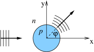
Figure 1: (Color online) An incident plane wave of electrons in bilayer graphene is scattered by a circular $n$-$p$ junction created by a gate-induced circular potential barrier $V(r)$. In the $n$ ($p$) region the Fermi energy lies in the conduction (valence) band.

In this Section we consider the scattering of an electron plane wave on a circular $n$-$p$ junction in bilayer graphene (see Fig.1). Our goal is to calculate the exact scattering wave function as a function of system parameters and to identify the characteristics of the flow of electrons inside the circular $p$ region. We will focus on the case when the radius of the circle is much larger then the electron wavelength, since in that regime we expect a correspondence between results of the quantum mechanical model and a simplified description based on principles of geometrical optics.

To model the two-dimensional electron flow in bilayer graphene, we use a two-component envelope function Hamiltonian which has been derived by McCann and Fal’koMcCann and Falko (2006). The derivation of this Hamiltonian starts from a simple tight-binding model of bilayer graphene, which contains only nearest-neighbor intralayer and interlayer hopping matrix elements. These hopping matrix elements are usually denotedCastro Neto et al. (2009); McCann et al. (2007) by $\gamma_{0}$ and $\gamma_{1}$, respectively. This tight binding model predicts that the valence and conduction bands of bilayer graphene are touching at the $K$ and $K^{\prime}$ points, i. e. at the two nonequivalent corners of the hexagonal Brillouin zone. The Fermi energy of undoped bilayer graphene lies exactly at the energy corresponding to these touching points. In the vicinity of the $K$ point, the dispersion relations describing the conduction and valence bands are both quadratic, $E_{\pm}(\text{\boldmath{$k$}})\approx\pm\hbar^{2}(\text{\boldmath{$k$}}-\text{\boldmath{$K$}})^{2}/2m$, where $m=\frac{2\hbar^{2}\gamma_{1}}{3a^{2}\gamma_{0}^{2}}\approx 0.054m_{0}$ is the effective mass. Here the $+$ ($-$) sign refers to the conduction (valence) band, $a$ is the lattice constant and $m_{0}$ is the free electron mass. In this low-energy regime the quasiparticle wave functions can be characterized by the eigenfunctions of the $2\times 2$ effective Hamiltonian

$$H_{0}=-\frac{1}{2m}\left[\begin{array}[]{cc}0&p_{-}^{2}\\ \vskip 6.0pt plus 2.0pt minus 2.0pt\cr p_{+}^{2}&0\end{array}\right],$$ (1)

where $p_{\pm}=(p_{x}\pm ip_{y})$. Note that this Hamiltonian describes the valence band and conduction band states simultaneously. Similar statements are true for the vicinity of the $K^{\prime}$ point. We note that the dispersion relation and the effective Hamiltonian becomes more complex if one includes second-nearest-neighbor interlayer hopping matrix elements in the tight-binding model. In particular, such terms lead to a trigonal warpingMcCann et al. (2007); McCann and Falko (2006); Cserti et al. (2007b) of the quasiparticle dispersion. We comment on the significance of trigonal warping in Section IV.

We model the gate-defined circular potential barrier by a step-like potential $V(r)=V_{0}\Theta(R-r)$, where $\Theta$ denotes the Heaviside function. Hence the complete Hamiltonian of the system under study is

$$H=H_{0}+V(r)\openone,$$ (2)

where $\openone$ is the $2\times 2$ unit matrix. The validity of this model will be discussed in Section IV. Note that the same model was used recently to calculate the lifetime of quasibound states in a similar systemMatulis and Peeters (2008).

We concentrate on the regime where the potential barrier forms an $n$-$p$ junction, i.e. the Fermi energy $E_{F}$ of the electrons lies between the Dirac point of the bulk and the top of the potential barrier ($0<E_{F}<V_{0}$). In this case, the region outside the circle of radius $R$ contains electrons in the conduction band ($n$-type), whereas the region inside the circle contains holes in the valence band ($p$-type).

Our aim is to consider the scattering of an incident electron plane wave coming from the $n$ region along the $x$-axis as shown in Fig. 1 and having energy $E_{F}$. Such an electron has the following two-component wave functionKatsnelson et al. (2006):

$$\phi(x,y)=e^{ik_{n}x}\frac{1}{\sqrt{2}}\left[\begin{array}[]{c}1\\[6.45831pt] -1\end{array}\right],$$ (3)

where $k_{n}=\sqrt{2mE_{F}}/\hbar$. In order to derive the wave function describing the scattering of this plane wave, we first treat the scattering of cylindrical waves and then utilize the fact that the plane wave $\phi(x,y)$ is a certain linear combination of cylindrical waves. Here we note that scattering theory has been used recently to predict transport properties of disorderedKatsnelson (2007); Kechedzhi et al. (2007); Adam and Das Sarma (2008); Culcer and Winkler (2009) and ballisticBraun et al. (2008) bilayer graphene structures.

The system has a circular symmetry around the origin, hence the Hamiltonian commutes with a pseudo angular momentum’ operator $J_{z}=-i\hbar\partial_{\varphi}+\hbar\sigma_{z}$, where $\partial_{\varphi}$ is the derivative with respect to the angular polar coordinate and $\sigma_{z}$ is the third Pauli matrix. The presence of this symmetry simplifies the forthcoming calculations.

Using the properties of Bessel functionsAbramowitz and Stegun (1972) it can be shown that in the $n$ region, for any integer $j$ the wave functions

$$\mathbf{h}_{j}^{(1)}(r,\varphi) = \left[\begin{array}[]{c}H^{(1)}_{j-1}(k_{n}r)e^{-i\varphi}\\[6.45831pt] H^{(1)}_{j+1}(k_{n}r)e^{i\varphi}\end{array}\right]{e^{ij\varphi}},$$ (4c)

$$\mathbf{h}_{j}^{(2)}(r,\varphi) = \left[\begin{array}[]{c}H^{(2)}_{j-1}(k_{n}r)e^{-i\varphi}\\[6.45831pt] H^{(2)}_{j+1}(k_{n}r)e^{i\varphi}\end{array}\right]{e^{ij\varphi}},$$ (4f)

$$\mathbf{k}_{j}(r,\varphi) = \left[\begin{array}[]{c}K_{j-1}(k_{n}r)e^{-i\varphi}\\[6.45831pt] K_{j+1}(k_{n}r)e^{i\varphi}\end{array}\right]{e^{ij\varphi}}$$ (4i)

are simultaneous eigenfunctions of $H$ and $J_{z}$, with eigenvalues $E_{F}$ and $\hbar j$, respectively. We denote the radial polar coordinate with $r$. Here $H_{m}^{(1)}$, $H_{m}^{(2)}$ and $K_{m}$ denote Hankel functions of first and second kind and the modified Bessel function which is bounded for large argumentsAbramowitz and Stegun (1972), respectively. There exists a solution similar to those in Eq. (4), containing the modified Bessel function $I_{m}$. We disregard it because $I_{m}$ diverges for large arguments. Analysis of the quantum mechanical current density in state $\mathbf{h}_{j}^{(1)}$ ($\mathbf{h}_{j}^{(2)}$) shows that it is an outgoing (incoming) cylindrical wave. On the other hand, $\mathbf{k}_{j}$ is an evanescent cylindrical wave which does not carry current in the radial direction.

Inside the circular $p$ region, the regular eigenfunctions of the Hamiltonian $H$ having energy $E_{F}$ are

$$\mathbf{j}_{j}(r,\varphi) = \left[\begin{array}[]{c}J_{j-1}(k_{p}r)e^{-i\varphi}\\[6.45831pt] -J_{j+1}(k_{p}r)e^{i\varphi}\end{array}\right]{e^{ij\varphi}},$$ (5c)

$$\mathbf{i}_{j}(r,\varphi) = \left[\begin{array}[]{c}I_{j-1}(k_{p}r)e^{-i\varphi}\\[6.45831pt] -I_{j+1}(k_{p}r)e^{i\varphi}\end{array}\right]{e^{ij\varphi}}.$$ (5f)

Here $k_{p}=\sqrt{2m(V_{0}-E_{F})}/\hbar$ and $j$ is an arbitrary integer. Similarly to the wave functions in the $n$ region, $\mathbf{j}_{j}$ and $\mathbf{i}_{j}$ are eigenfunctions of $J_{z}$ with an eigenvalue $\hbar j$. We disregard other eigenfunctions of $H$ which are divergent at the origin.

Now we consider the scattering of a single incoming cylindrical wave, $\mathbf{h}^{(2)}_{j}$. Since $[H,J_{z}]=0$, the pseudo angular momentum does not change during the scattering process, therefore the complete wave function describing the scattering can be written as

$$\psi^{(n)}_{j} = \mathbf{h}^{(2)}_{j}+S_{j}\mathbf{h}^{(1)}_{j}+A_{j}\mathbf{k}_{j},$$ (6a)

$$\psi^{(p)}_{j} = B_{j}\mathbf{j}_{j}+C_{j}\mathbf{i}_{j},$$ (6b)

in the $n$ and $p$ regions, respectively. The coefficients $S_{j}$, $A_{j}$, $B_{j}$ and $C_{j}$ have to be determined from the boundary conditions at the interface of the NPJ: the wave functions and their derivatives have to be continuous at $r=R$. Due to the two-component nature of the wavefunctions, the two boundary conditions result in an inhomogeneous linear system with four equations and the four coefficients as unknowns. This system can be solved analytically.

Having the coefficients $S_{j}$, $A_{j}$, $B_{j}$ and $C_{j}$ in hand, one can determine the wave function describing the scattering of the plane wave $\phi$ in Eq. (3). Making use of the fact thatAbramowitz and Stegun (1972)

$$e^{ikx}=\sum_{m\in\mathbb{Z}}i^{m}J_{m}(kr)e^{im\varphi},$$ (7)

it can be shown that the plane wave $\phi$ can be written as a linear combination of incoming and outgoing cylindrical waves:

$$\phi=\frac{1}{i\sqrt{8}}\sum_{j\in\mathbb{Z}}i^{j}\left(\mathbf{h}^{(1)}_{j}+\mathbf{h}^{(2)}_{j}\right).$$ (8)

This expansion allows us to use the coefficients determined from the analysis of partial waves to derive the wave function describing the scattering of the plane wave. In the $n$ region,

$$\psi^{(n)}=\phi+\frac{1}{i\sqrt{8}}\sum_{j\in\mathbb{Z}}i^{j}\left[(S_{j}-1)\mathbf{h}^{(1)}_{j}+A_{j}\mathbf{k}_{j}\right],$$ (9)

and in the $p$ region

$$\psi^{(p)}=\frac{1}{i\sqrt{8}}\sum_{j\in\mathbb{Z}}i^{j}\left(B_{j}\mathbf{j}_{j}+C_{j}\mathbf{i}_{j}\right).$$ (10)

The complete wave function $\psi$ is constructed by tailoring $\psi^{(n)}$ and $\psi^{(p)}$. It is built up from cylindrical waves having energy $E_{F}$, therefore $\psi$ is also an energy eigenstate with energy $E_{F}$. Since the cylindrical waves fulfill the boundary conditions at $R$, $\psi$ also fulfills them. Finally, since in the $n$ region $\psi$ contains only the plane wave and outgoing and evanescent cylindrical waves (no incoming wave), we conclude that $\psi$ is the wave function which describes the scattering of the incident plane wave.

Figure 2: (Color online) The spatial dependence of the intensity of the wave function $|\psi(\text{\boldmath{$r$}})|^{2}$ is plotted in the scattering area. Here $k_{n}R=300$, and $k_{p}R=300$ corresponding to $n=-1$. The solid (dashed) line corresponds to the caustic for $p=1$ ($p=2$), where $p$ denotes the number of chords inside the NPJ Cserti et al. (2007).

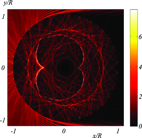
Figure 3: (Color online) The same as in Fig. 2 with $k_{n}R=200$ and $k_{p}R=300$ corresponding to $n=-1.5$.

Numerical results for the spatial dependence of the magnitude of the complete scattering state ($|\psi(\text{\boldmath{$r$}})|^{2}$) are shown in Fig. 2 and Fig. 3 for two different set of parameters. In both cases, well-defined patterns of the electron flow can be identified, the wave function magnitude is sharply peaked close to the solid curve. This effect is almost identical to the one predicted for circular NPJs of monolayer grapheneCserti et al. (2007). As we will argue in Section III, the geometrical optics model developed in Ref. Cheianov et al., 2007 and Ref. Cserti et al., 2007 for single layer graphene is also applicable for bilayer with certain restrictions. According to the referred theories, the refraction of the incident electrons is governed by Snell’s law with a negative refractive index. After the refraction, the electrons enter the $p$ region of the junction, and the envelope of the electron rays form a caustic. These caustics can be identified in the quantum mechanical charge density, as it is revealed by Figs. 2 and 3.

Despite the apparent similarities of the monolayer and bilayer case, the analogy is not complete. In a circular monolayer NPJ the charge density is maximal close to the meeting point of the two caustic lines, which means that the interface between the $n$ and $p$ regions provides strong focusing of the incident electronsCserti et al. (2007). This feature is missing in our results for the bilayer. In Section III we will show that the absence of focusing is connected to a general characteristic of interband (Klein) tunneling in bilayer graphene.

III Transmission in a planar $n$-$p$ junction

In this section we study the refraction of electron plane waves at a planar $n$-$p$ junction of bilayer graphene. We derive the counterpart of Snell’s law for this system, and calculate how the probability of transmission depends on the propagation direction of the incident electron. The obtained results will be used to explain our findings for the circular NPJ (Section II).

The studied system consists of a sheet of bilayer graphene in the $x$-$y$ plane which is $n$-type for $x<0$ and $p$-type for $x>0$. The electrostatic potential which creates these regions is modelled by a step-like function $V(x,y)=V_{0}\Theta(x)$. We consider a conduction electron plane wave incident from the $n$ side of the junction. We assume that the propagation direction of the plane wave is given by the angle $\alpha\in[-\pi/2,\pi/2]$, and it has energy $E_{F}$ ($0<E_{F}<V_{0}$).

To derive the Snell’s law for planar $n$-$p$ junction of bilayer graphene we follow Ref. Cheianov et al., 2007. The length of the wave vector in the $n$ ($p$) region is $k_{n}$ ($k_{p}$), and the length of the corresponding group velocity is $v_{n}$ ($v_{p}$). (We assume that the plane wave is refracted, and do not consider the case of total reflection here.) The incident electron has the velocity $v_{n}(\cos\alpha,\sin\alpha)$ and wave vector $k_{n}(\cos\alpha,\sin\alpha)$. At the interface this electron is partially reflected with velocity $v_{n}(-\cos\alpha,\sin\alpha)$ and wave vector $k_{n}(-\cos\alpha,\sin\alpha)$. We denote the direction of propagation of the refracted wave by $\beta$, hence the velocity of the refracted wave is $v_{p}(\cos\beta,\sin\beta)$. Since the refracted wave is in the valence band, its velocity is antiparallel with its wave vector, and thus the corresponding wave vector is $k_{p}(-\cos\beta,-\sin\beta)$. The translational invariance of the system along the $y$ direction implies that the $y$ component of the wave vector must not change during the refraction, i.e. $k_{n}\sin\alpha=-k_{p}\sin\beta$, which results in Snell’s law with a negative refractive index $n=-k_{p}/k_{n}$,

$$\frac{\sin\alpha}{\sin\beta}=n<0.$$ (11)

This form of Snell’s law is identical to the one found for monolayer graphene NPJs. Consequently, the mathematical formula describing the caustic lines formed by the electron rays in a circular bilayer NPJ is also identical to the one derived for the monolayer case. This formula is given for the monolayer in Eq. (9) of Ref. Cserti et al., 2007, and it has been used to plot the solid curves in Figs. 2 and 3. The correspondence between the description of the electron flow in terms of quantum mechanics and geometrical optics is apparent from the figures: the high-density regions of the quantum mechanical wave functions are condensed in the vicinity of the caustic line.

We further investigate the refraction of electrons at the $n$-$p$ interface by calculating the probability of transmission as the function of the angle of incidence $\alpha$. The system is modelled by the Hamiltonian $H=H_{0}+V_{0}\Theta(x)$. The wave functions at the $n$ and $p$ regions can be constructed using the results of Ref. Katsnelson et al., 2006. In the $n$ region, the incident, reflected and evanescent modes are given by

$$\psi_{\rm inc}(x,y) = e^{ik_{ny}y}e^{ik_{nx}x}\left[\begin{array}[]{c}1\\[6.45831pt] -e^{2i\alpha}\end{array}\right],$$ (12c)

$$\psi_{\rm refl}(x,y) = e^{ik_{ny}y}e^{-ik_{nx}x}\left[\begin{array}[]{c}1\\[6.45831pt] -e^{-2i\alpha}\end{array}\right],$$ (12f)

$$\psi_{\rm ev,n}(x,y) = e^{ik_{ny}y}e^{\kappa_{n}x}\left[\begin{array}[]{c}1\\[6.45831pt] h(\alpha)\end{array}\right],$$ (12i)

where $k_{ny}=k_{n}\sin\alpha$, $k_{nx}=k_{n}\cos\alpha$, $\kappa_{n}=k_{n}\sqrt{1+\sin^{2}\alpha}$ and $h(\alpha)=(\sqrt{1+\sin^{2}\alpha}-\sin\alpha)^{2}$. In the $p$ region, the refracted and the evanescent waves are

$$\psi_{\rm refr}(x,y) = e^{ik_{ny}y}e^{-ik_{px}x}\left[\begin{array}[]{c}1\\[6.45831pt] e^{2i\beta}\end{array}\right],$$ (13c)

$$\psi_{\rm ev,p}(x,y) = e^{ik_{ny}y}e^{-\kappa_{p}x}\left[\begin{array}[]{c}1\\[6.45831pt] -1/h(\beta+\pi)\end{array}\right].$$ (13f)

Here $k_{px}=k_{p}\cos\beta$ and $\kappa_{p}=k_{p}\sqrt{1+\sin^{2}\beta}$. Note that the refraction angle $\beta$ has to be determined from Snell’s law [Eq. (11)].

The wave function describing the reflection-refraction process in the $n$ region is $\psi_{n}=\psi_{\rm inc}+r\psi_{\rm refl}+a\psi_{\rm ev,n}$, whereas in the $p$ region it is $\psi_{p}=t\psi_{\rm refr}+b\psi_{\rm ev,p}$. One has to determine the coefficients $r$, $a$, $t$ and $b$ from the boundary conditions which match the wavefunctions and their derivatives at the interface $x=0$. The transmission probability as a function of the angle of incidence is

$$T(\alpha) = |t(\alpha)|^{2}\frac{\left<\psi_{\rm refr}|v_{x}|\psi_{\rm refr}\right>}{\left<\psi_{\rm inc}|v_{x}|\psi_{\rm inc}\right>}\mbox{, where}$$ (14)

$$v_{x} = \frac{i}{\hbar}[H,x]=-\frac{1}{m}\left[\begin{array}[]{cc}0&p_{-}\\ p_{+}&0\end{array}\right]$$ (17)

is the $x$-component of the current operator. Similarly, we found that $R(\alpha)=|r(\alpha)|^{2}=1-T(\alpha)$.

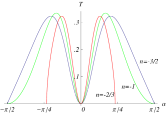
Figure 4: (Color online) Angular dependence of transmission probability through a planar NPJ of bilayer graphene. The corresponding values of the refractive index $n$ are shown in the figure.

In Fig. 4 we plot $T(\alpha)$ for three different values of the refractive index. A characteristic feature of all the three cases is the absence of transmission for perpendicular incidence, $T(0)=0$. This behavior has been predicted and explained with the chiral nature of the quasiparticles of bilayer grapheneKatsnelson et al. (2006). With the help of Fig. 5 we argue that the absence of transmission at perpendicular incidence is responsible for the complete suppression of focusing in the circular junction we studied in Section II. Fig. 5 shows several electron rays approaching the circular $p$ region and being refracted at the $n$-$p$ interface. An incoming electron ray can be characterized by its impact factor $b$, which is the distance between the incoming ray and the optical axis (defined as the line containing the horizontal diameter of the circular $p$ region, see Fig. 4 of Ref. Cserti et al., 2007). Note that the impact factor of rays entering the $p$ region is between $-R$ and $R$. The angle of incidence, i.e. the angle between the incoming electron ray and the local normal vector of the interface at the point of incidence, can be calculated from simple trigonometry: $\alpha(b)={\rm arcsin}\frac{b}{R}$. From this result one can express (i) the propagation direction of the refracted ray using Snell’s law in Eq. (11), and (ii) the probability of transmission (=refraction) as a function of the impact parameter $T(b)$, by combining the results for $T(\alpha)$ and $\alpha(b)$. In Fig. 5 the darkness of the refracted electron rays reflects the transmission probability $T(b)$. The figure indicates that the electron rays approaching the junction in the close vicinity of the optical axis does not have an appreciable probability of transmission at the interface, which leads to the complete suppression of the focusing effect (cf. Fig. 5 of Ref. Cserti et al., 2007).

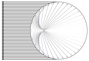
Figure 5: (Color online) Refraction of electron rays at the interface of the $n$-$p$ junction. The darkness of the refracted rays reflects the transmission probability: a white ray corresponds to $T=0$, and a black ray would correspond to $T=1$. The dashed curve shows the shape of the caustic derived from Snell’s lawCserti et al. (2007). Only the rays with no internal reflections are displayed. Here the refractive index is $n=-1$.

An other remarkable feature of the transmission functions plotted in Fig. 4 is that transmission is significant ($\geq 0.1$) in a wide range between perpendicular ($\alpha=0$) and nearly parallel ($|\alpha|\approx\pi/2$) incidence. With respect to the circular junction shown in Fig. 5, it means that electron rays hitting the NPJ further from the optical axis have a significant probability to be refracted, and hence, to form caustics along the dashed line of Fig. 5. This analysis built on the geometrical optics approach and the transmission probability calculations for the planar junction provides a qualitative explanation of the presence of the well-defined wave function patterns presented in Figs. 2 and 3.

IV Discussion and Summary

During the analysis of circular and planar NPJs, we modelled the electrostatic potential as a step-like function of position which does not couple different valleys. This assumption is justified if $a\ll d\ll\lambda_{n},\lambda_{p}$, where $a$ is the lattice constant, $d$ is the characteristic length describing the width of the transition region between the $n$ and $p$ sides of the junction and $\lambda_{n}$, $\lambda_{p}$ are the de Broglie wavelengths of the considered quasiparticles in the $n$ and $p$ regions. The first relation $a\ll d$ ensures the absence of intervalley scattering at the interface, and the second relation $d\ll\lambda_{n},\lambda_{p}$ justifies the usage of a step-like potential in our model.

Since the geometrical optics model is expected to capture the main features of electron flow patterns only when the wavelength of the electrons is much shorter then the size of the system, the conditions $k_{n}R,k_{p}R\gg 1$ has to be fulfilled to observe a pronounced caustic formation effect.

In the model Hamiltonian in Eq. (2) we neglected the trigonal warping termMcCann and Falko (2006); McCann et al. (2007) and used an approximate effective Hamiltonian which results in a quadratic dispersion relation. In bilayer graphene trigonal warping is strong only at very low energies, when $E_{F}<\gamma_{1}(\gamma_{3}/\gamma_{0})^{2}/4\approx 1.15$meV. Here $\gamma_{0}$, $\gamma_{1}$ and $\gamma_{3}$ are hopping matrix elements of the standard tight-binding model of bilayer grapheneMcCann and Falko (2006); McCann et al. (2007), and we used estimates for them from the review of Castro Neto et al.Castro Neto et al. (2009) For larger energies, the dispersion relation is dominantly quadratic up to an energy $E_{F}=\gamma_{1}/2\approx 200$meV, where it crosses over to a mostly linear dispersion.McCann and Falko (2006); McCann et al. (2007) Therefore our model should give a good description of quasiparticles having energies between $1.15$meV and $200$meV.

To give a numerical example of parameters which fulfill the above criteria, we consider a bilayer graphene circular NPJ with Fermi energy $E_{F}=10$meV, gate potential $V_{0}=20$meV, transition region width $d=10$nm and $p$ region radius $R=1\mu$m. Then $k_{n}=k_{p}\approx 0.12$nm^-1, $\lambda_{n}=\lambda_{p}\approx 53$nm, $k_{n}R=k_{p}R\approx 118$ and the refractive index $n=-1$. For these experimental parameters the model we used is expected to give a good description of electron dynamics in the circular bilayer NPJ, and the relation $k_{n}R=k_{p}R\approx 118\gg 1$ is expected to ensure the strong caustic formation effect in this system.

Finally, we summarize some experimental results which support the feasibility of electron optics devices in graphene in general. Control of electron flow in a ballistic two-dimensional electron system by means of gate-defined potential barriers as refractive elements has been realized nearly two decades agoSpector et al. (1990). Direct imaging of the electron flow in a two-dimensional electron system has also been carried out applying scanning gate techniquesTopinka et al. (2000, 2001). Scanning tunneling microscopy has been used to show that oscillations of the local density of states around a static impurity can be refocused to a remote locationManoharan et al. (2000). To realize similar experiments making use of the negative refraction index in graphene, a trivial prerequisite is the ability to fabricate gate-defined tunable NPJs, which has already been reported by several groupsÖzyilmaz et al. (2007); Huard et al. (2007); Liu et al. (2008); Williams et al. (2007); Gorbachev et al. (2008); Stander et al. (2009); Young and Kim (2009).

In conclusion, we have carried out a theoretical analysis of electron dynamics in circular NPJs of bilayer graphene. We demonstrated that such a system might be used to control the flow of electrons, similarly to previously realized and proposed electron optics devices. We have pointed out similarities and differences between electron dynamics in the circular NPJ of bilayer and monolayer graphene. In both devices, electron paths form caustics inside the circular $p$ region, and the form of these caustics can be described with a geometrical optics model based on the concept of negative refractive index. The major difference is that the strong focusing of electrons, which is a characteristic of the monolayer device, is completely absent in the bilayer. Our findings are explained in terms of the angular dependence of transmission probability at a planar NPJ.