Numerical Construction of Magnetosphere with Relativistic Two-fluid Plasma Flows

Abstract

We present a numerical model in which a cold pair plasma is ejected with relativistic speed through a polar cap region and flows almost radially outside the light cylinder. Stationary axisymmetric structures of electromagnetic fields and plasma flows are self-consistently calculated. In our model, motions of positively and negatively charged particles are assumed to be determined by electromagnetic forces and inertial terms, without pair creation and annihilation or radiation loss. The global electromagnetic fields are calculated by the Maxwell’s equations for the plasma density and velocity, without using ideal MHD condition. Numerical result demonstrates the acceleration and deceleration of plasma due to parallel component of the electric fields. Numerical model is successfully constructed for weak magnetic fields or highly relativistic fluid velocity, i.e, kinetic energy dominated outflow. It is found that appropriate choices of boundary conditions and plasma injection model at the polar cap should be explored in order to extend present method to more realistic pulsar magnetosphere, in which the Poynting flux is dominated.

1 INTRODUCTION

A global structure of pulsar magnetosphere is one of key issues to understanding energy outflow to the exterior. The numerical model has been successfully developed in the past decade, although the basic equation was already derived in the early days of pulsar theory. Extensive reviews are available in some books (e.g, Michel (1991); Beskin et al. (1993); Mestel (1999)). Contopoulos et al. (1999) calculated the stationary axially symmetric magnetosphere based on the force-free approximation. They for the first time showed a solution with dipole magnetic field lines near a neutron star, which smoothly pass through the light cylinder to the wind region at infinity. In the model, there is a current sheet flowing on the separatrix and equator outside the light cylinder. The magnetosphere model is subsequently explored in detail by several authors; some physical properties represented by the solution (Ogura & Kojima, 2003), the Y-point singularity between open and closed field lines on the equator (Uzdensky, 2003; Timokhin, 2006), the electromagnetic luminosity in high numerical resolution (Gruzinov, 2005, 2006). Numerical construction of the magnetosphere around an aligned rotator is also performed using time-dependent codes with the force-free and MHD approximations (Komissarov, 2006; McKinney, 2006). A stationary state, which is very similar to the solution given by Contopoulos et al. (1999), is obtained with certain initial and boundary conditions. The approach is extended to an oblique rotator by 3D simulation codes (Spitkovsky, 2006; Kalapotharakos & Contopoulos, 2008).

An ideal MHD condition $\vec{E}=\vec{B}\times\vec{v}/c$ is used to determine the electric field in these calculations irrespective of the numerical methods. Consequently, two electromagnetic field vectors are always orthogonal $\vec{B}\cdot\vec{E}=0$, and the parallel component of $\vec{E}$ along the plasma motion vanishes everywhere. This condition holds if the plasma density much exceeds the Goldreich-Julian density (Goldreich & Julian, 1969). The global structure based on the force-free and MHD approximations is obviously a good step to understanding the whole magnetosphere. However, it is important to study how and where the condition breaks down, and how this changes the electromagnetic field structure and plasma behavior. An alternative approach, in which the ideal MHD condition is relaxed, is necessary to address these problems. Breakdown of ideal MHD condition in the pulsar magnetosphere is qualitatively pointed out in the literature, e.g, (Mestel & Shibata, 1994; Goodwin et al., 2004). It is our purpose to further study the problem by actual modeling. It is necessary to determine the electric fields from the distribution of the charge density, since $\vec{E}=\vec{B}\times\vec{v}/c$ is no longer used. The electric acceleration or deceleration of fluids will be allowed elsewhere, since $\vec{v}\cdot\vec{E}\neq 0$. The location may be important to the observation.

In this paper, we present an approach based on a two-fluid plasma consisting of positively and negatively charged particles. In this approach, the electromagnetic fields are modeled by Maxwell’s equations with a plasma source. Resultant electric fields are not in general perpendicular to magnetic fields $\vec{B}\cdot\vec{E}\neq 0$, i.e, breakdown of ideal MHD condition. The stream lines of the plasma flows are not a priori assumed to coincide with the magnetic field lines. The plasma flows are determined by equation of motion under the electromagnetic forces. In this paper, we consider a simple plasma model, a cold dissipationless plasma, in which thermal pressure, pair creation or annihilation and radiation loss are neglected. If we further neglect the inertial terms in equations of motion, then we have the force-free and MHD conditions (Goodwin et al., 2004). We here keep the inertial terms, in order to model the magnetosphere taken into account one of non-ideal MHD effects. We also assume stationary axisymmetric states in the electromagnetic fields and the plasma flows. However, the azimuthal component of a vector is not zero in general. For example, a toroidal magnetic field $B_{\phi}$ can be produced by poloidal currents $\vec{j}_{p}=(j_{r},j_{\theta})$, in the spherical coordinates $(r,\theta,\phi)$. This approach can be naturally extended to include other physical mechanisms in the future. This paper is, therefore, the first step towards including more physical processes.

This paper is organized as follows. In section 2, we discuss our numerical method to solve electromagnetic fields and fluid streams in two-dimensional meridian plane. The relevant boundary conditions are also given. A model of plasma injection is given at the inner boundary, a polar cap region. The angular dependence of the injection rates is different between positively and negatively charged particles, but the total is the same. The total current from the polar cap is therefore zero. This provides a model to construct magnetosphere with charge-separated plasma flow. This choice of the injection model is not unique. In section 3, we show our results of the global structure. Section 4 contains our conclusions.

2 ASSUMPTIONS AND EQUATIONS

2.1 Electromagnetic fields and plasma flows

Axially symmetric electromagnetic fields in the stationary state are expressed by three functions $\Phi(r,\theta)$,$G(r,\theta)$,$S(r,\theta)$ as

$$\vec{E} = -\vec{\nabla}\Phi,$$ (1)

$$\vec{B} = \frac{1}{R}\vec{\nabla}G\times\vec{e}_{\phi}+\frac{S}{R}\vec{e}_{\phi},$$ (2)

where we use spherical coordinate $(r,\theta,\phi)$ and $R=r\sin\theta$. It is convenient to use the non-corotational potential $\Psi=\Phi-\Omega G/c$, where $\Omega$ is angular velocity of a central star. Maxwell equations with charge density $\rho_{e}$, and poloidal and toroidal components of current $(\vec{j}_{p},j_{\phi})$ are given by

$${\mathcal{D}}G=-\frac{4\pi}{c}Rj_{\phi},$$ (3)

$$\frac{1}{R}\vec{\nabla}S\times\vec{e}_{\phi}=\frac{4\pi}{c}\vec{j}_{p},$$ (4)

$$\nabla^{2}\Psi=-4\pi\left(\rho_{e}-\frac{\Omega R}{c^{2}}j_{\phi}\right)-\frac{2\Omega}{cr^{2}}\left(r\frac{\partial G}{\partial r}+\cot\theta\frac{\partial G}{\partial\theta}\right),$$ (5)

where operators ${\mathcal{D}}$ and $\nabla^{2}$ in spherical coordinate are given by

$${\mathcal{D}}=\frac{\partial^{2}}{\partial r^{2}}+\frac{\sin\theta}{r^{2}}\frac{\partial}{\partial\theta}\left(\frac{1}{\sin\theta}\frac{\partial}{\partial\theta}\right),$$ (6)

$$\nabla^{2}=\frac{1}{r^{2}}\frac{\partial}{\partial r}\left(r^{2}\frac{\partial}{\partial r}\right)+\frac{1}{r^{2}\sin\theta}\frac{\partial}{\partial\theta}\left(\sin\theta\frac{\partial}{\partial\theta}\right).$$ (7)

We adopt a treatment in which the plasma is modeled as a two-component fluid. Each component, consisting of positively or negatively charged particles, is described by a number density $n_{\pm}$ and velocity $\vec{v}_{\pm}=\vec{v}_{\pm p}+v_{\phi}\vec{e}_{\phi}$. Note that the proper density $n_{\pm}^{\ast}$ is related with the lab-frame density $n_{\pm}$ by $n_{\pm}^{\ast}=n_{\pm}/\gamma_{\pm}$, where $\gamma_{\pm}$ is a Lorentz factor $\gamma_{\pm}=(1-(v_{\pm}/c)^{2})^{-1/2}$ (e.g, Goodwin et al. (2004)). We assume that the positive particle has mass $m$ and charge $q$, while the negative one has mass $m$ and charge $-q$. The charge density and electric current are given in terms of $n_{\pm}$ and $\vec{v}_{\pm}$ as

$$\rho_{e} = q(n_{+}-n_{-}),$$ (8)

$$\vec{j} = q(n_{+}\vec{v}_{+}-n_{-}\vec{v}_{-}).$$ (9)

Continuity equation for each component in the stationary axisymmetric conditions is

$$0=\vec{\nabla}\cdot(n_{\pm}\vec{v}_{\pm})=\vec{\nabla}\cdot(n_{\pm}\vec{v}_{\pm p}).$$ (10)

The poloidal velocity components $\vec{v}_{\pm p}$ are satisfied by introducing a stream function $F_{\pm}(r,\theta)$ as

$$n_{\pm}\vec{v}_{\pm p}=\frac{1}{R}\vec{\nabla}F_{\pm}\times\vec{e}_{\phi}.$$ (11)

From the definition, the number density is given by

$$n_{\pm}=\frac{|\nabla F_{\pm}|}{R(v_{\pm r}^{2}+v_{\pm\theta}^{2})^{1/2}}.$$ (12)

From eqs.(9) and (11), the current function $S$ in eq.(4) can be solved as

$$S=\frac{4\pi q}{c}(F_{+}-F_{-}).$$ (13)

The electromagnetic force is dominant so that collision, thermal pressure and gravity are ignored. The interaction between two-component fluids is assumed only through the global electromagnetic fields. The equation of motion for each component with mass $m$ and charge $\pm q$ in the stationary state is given by

$$\left(\vec{v}_{\pm}\cdot\vec{\nabla}\right)\gamma_{\pm}\vec{v}_{\pm}=\pm\frac{q}{m}\left[\vec{E}+\frac{\vec{v}_{\pm}}{c}\times\vec{B}\right].$$ (14)

By adding and subtracting equations (14) for two components, we have an equation of one-fluid bulk motion and a generalized Ohm’s law. See e.g, (Melatos & Melrose, 1996; Goodwin et al., 2004) for the detailed discussion. We do not follow such a treatment, but rather solve eq.(14) for each component. Using the identity $(\vec{v}\cdot\vec{\nabla})\gamma\vec{v}$ $=(\vec{\nabla}\times\gamma\vec{v})\times\vec{v}+\vec{\nabla}\gamma c^{2}$, we find two conserved quantities along each stream line, corresponding to axially symmetric and stationary conditions. They are generalized angular momentum $J_{\pm}$ and Bernoulli integral $K_{\pm}$, which are obtained by the azimuthal component of eq.(14) and a scalar product of $\vec{v}$ and eq.(14) (Mestel, 1999). Their explicit expressions are given by

$$J_{\pm}=\gamma_{\pm}v_{\pm\phi}R\pm\frac{q}{mc}G,$$ (15)

$$K_{\pm}=\gamma_{\pm}\pm\frac{q}{mc^{2}}\Phi.$$ (16)

These quantities depend on the stream functions $F_{\pm}$ only, and the spatial distributions are therefore determined by $F_{\pm}$ which is specified at the injection point in our model. The convenient form for the third component of eq.(14) is the azimuthal component of a cross product of $\vec{v}$ and eq.(14). This means a perpendicular component to the stream lines, which is given by

$${\mathcal{D}}F_{\pm}=\vec{\nabla}\ln\left(\frac{n_{\pm}}{\gamma_{\pm}}\right)\cdot\vec{\nabla}F_{\pm}+\frac{c^{2}n_{\pm}^{2}R^{2}}{\gamma_{\pm}}\left(K_{\pm}^{\prime}-\frac{v_{\pm\phi}}{c^{2}R}J_{\pm}^{\prime}\right)\pm\frac{q}{mc}\frac{n_{\pm}}{\gamma_{\pm}}S,$$ (17)

where $J_{\pm}^{\prime}$ and $K_{\pm}^{\prime}$ are derivatives of $J_{\pm}$ and $K_{\pm}$ with respect to $F_{\pm}$. Using $\vec{\nabla}J_{\pm}=J_{\pm}^{\prime}\vec{\nabla}F_{\pm}$, $\vec{\nabla}K_{\pm}=K_{\pm}^{\prime}\vec{\nabla}F_{\pm}$ and eq.(12), eq.(17) can be written in an alternative form

$${\mathcal{D}}F_{\pm}=\left[\vec{\nabla}\ln\left(\frac{n_{\pm}}{\gamma_{\pm}}\right)+\frac{c^{2}}{\gamma_{\pm}(v_{\pm r}^{2}+v_{\pm\theta}^{2})}\left(\vec{\nabla}K_{\pm}-\frac{v_{\pm\phi}}{c^{2}R}\vec{\nabla}J_{\pm}\right)\right]\cdot\vec{\nabla}F_{\pm}\pm\frac{q}{mc}\frac{n_{\pm}}{\gamma_{\pm}}S.$$ (18)

The stream function can not be defined in corotating region, where poloidal components of the velocity vanish, and the expression (11) is no longer used. Instead, the charge density $\rho_{e\ast}$ and current $\vec{j}_{\ast}$ are given in terms of the corotating condition $\Phi=\Omega G/c$, $\vec{j}_{\ast}=\rho_{e\ast}\Omega R\vec{e}_{\phi}$. From eq.(5), the corotating charge density is given by

$$4\pi\rho_{e\ast}=\frac{2c\Omega}{(c^{2}-\Omega^{2}R^{2})R}\left(\sin\theta\frac{\partial G}{\partial r}+\frac{\cos\theta}{r}\frac{\partial G}{\partial\theta}\right).$$ (19)

Three velocity components, Lorentz factor and number density are determined by eq.(12) and two integrals (15),(16), if four functions $G$, $\Psi$ and $F_{\pm}$ are known. The charge density (8) and current (9) are calculated from these fluid quantities of both species. In the corotating region, they are given by corotating charge density and current. Irrespective of the spatial region, the source terms of partial differential equations for $G$, $\Psi$ and $F_{\pm}$ depend on themselves in a non-linear manner. Some iterative methods are needed to self-consistently solve a set of eqs.(3),(5) and (18). There is no established method so far to solve nonlinearly coupled equations, so that our numerical procedure is rather primitive. Initial guess for these functions is assumed, say $G^{(0)}$, $\Psi^{(0)}$ and $F_{\pm}^{(0)}$. Using these functions, the source terms are calculated, and a new set of functions $G^{(1)}$, $\Psi^{(1)}$ and $F_{\pm}^{(1)}$ are solved from these source terms with appropriate boundary conditions. The procedure is repeated until the convergence, say, $|G^{(n+1)}-G^{(n)}|$, $|\Psi^{(n+1)}-\Psi^{(n)}|$, $|F_{\pm}^{(n+1)}-F_{\pm}^{(n)}|<\varepsilon$, where $\varepsilon$ is a small number. The iteration scheme may not necessarily lead to a convergent solution, since there is no mathematical proof.

In order to examine our numerical scheme, we have performed a test for the split-monopole case, for which an analytic solution is known (Michel, 1973). The non-corotational electric potential in the solution is zero everywhere, so that the condition $\Psi=0$ is used and a reduced system of $G$ and $F_{\pm}$ is checked. These functions are numerically solved by a finite difference method with appropriate boundary conditions in the upper half plane. Results for the convergence to the solution are given in Table 1. Two types of initial trial functions and two different grid numbers are used. Deviation from the analytic solution is shown by a norm $\|\delta f\|_{n}$, which is evaluated at all grid points as $\|\delta f\|_{n}=\left[\sum(f^{(n)}(r_{i},\theta_{j})-f^{\ast}(r_{i},\theta_{j}))^{2}\right]^{1/2}/\left[\sum(f^{\ast}(r_{i},\theta_{j}))^{2}\right]^{1/2}$, where $f^{\ast}$ is the analytic solution and $f^{(n)}$ is numerical result after $n$ iterations. We have repeated until the relative error $\varepsilon=1\times 10^{-3}$ in this test problem. We have started from $G^{(0)}=0$, so that $\|\delta G\|_{0}=1$. The initial choice of $G^{(0)}$ is not so important, since the numerical solution approaches the analytic one at the first step. On the other hand, the choice of initial guess for $F_{\pm}$ is important. It is not easy to set large deviation at the initial step, since the function $F_{\pm}$ should be monotonic. If there is a maximum or minimum, where $|\nabla F_{\pm}|=0$ inside the numerical domain, the flow vanishes $nv_{p}=0$. This causes a numerical difficulty at that point. From the monotonic nature consistent with the boundary conditions, the initial norm $\|\delta F_{\pm}\|_{0}$ can not be large. Table 1 shows that the numerical solutions successfully converge on the analytic ones within certain errors. Convergence factor $\varepsilon$ does not exactly correspond to deviation from true solution, but gives an estimate. The true solution is not known in most problems, and the deviation can not be calculated. The convergence factor $\varepsilon$ can be regarded as error estimate.

Table 1: Convergence test

Model	grid	$\|\delta G\|_{0}$	$\|\delta F_{+}\|_{0}$	$\|\delta F_{-}\|_{0}$	$\|\delta G\|_{N}$	$\|\delta F_{+}\|_{N}$	$\|\delta F_{-}\|_{N}$
A1	150 $\times$ 50	1.0	0.15	0.15	1.4 $\times$ 10-3	1.3 $\times$ 10-2	1.1 $\times$ 10-2
A2	300 $\times$ 100	1.0	0.15	0.15	4.1 $\times$ 10-4	7.4 $\times$ 10-3	5.6 $\times$ 10-3
B1	150 $\times$ 50	1.0	0.25	0.25	2.5 $\times$ 10-3	1.6 $\times$ 10-2	1.2 $\times$ 10-2
B2	300 $\times$ 100	1.0	0.25	0.25	9.1 $\times$ 10-4	7.8 $\times$ 10-3	5.2 $\times$ 10-3

2.2 Boundary conditions

We assume that the axially symmetry around a polar axis and the reflection symmetry across an equator. The numerical domain in the spherical coordinate $(r,\theta)$ is $r_{0}\leq r\leq r_{1}$, $0\leq\theta\leq\pi/2$. The inner and outer radii in our calculations are $r_{0}=r_{L}/5$ and $r_{1}=5r_{L}$, where $r_{L}=c/\Omega$ is the distance to the light cylinder. Figure 1 schematically represents the numerical domain. The functions at the inner boundary $r_{0}$ are closely related with plasma injection model, which is separately discussed in the next subsection. We here discuss the boundary conditions at the axis, equator and outer radius.

We solve the magnetic flux function $G$ in the upper half plane between $r_{0}$ and $r_{1}$, which is the region enclosed by a curve $PBRQP$ in Fig.1. Poloidal magnetic field at the inner boundary $r_{0}$, i.e, on $PB$ is dipole, so that we impose the condition, $G=\mu\sin^{2}\theta/r_{0}$, where $\mu$ is the magnetic dipole moment. The plasma is injected through a polar cap region $0\leq\theta\leq\theta_{0}$ at $r_{0}$, $PA$ in Fig.1. A curve $AL$ represents the last open magnetic field line. All the field lines originated from a point with $\theta\leq\theta_{0}$ at $r_{0}$ extend to infinity, whereas those from $\theta>\theta_{0}$ are closed. The point $L$ is $(r_{L},\pi/2)$. The last open line is given by $G_{0}=\mu\sin^{2}\theta_{0}/r_{0}$. For purely dipolar field, the polar cap region and critical field line are given by $\sin^{2}\theta_{0}=r_{0}/r_{L}$ and $G_{0}=\mu/r_{L}$. These values in our numerical model are not known a priori, but are determined simultaneously with the global structures. The boundary condition on the equator $\theta=\pi/2$ is $\partial G/\partial\theta=0$ inside the light cylinder, i.e, on $BL$ in Fig.1, while outside it $G=G_{0}$. This condition on the equator means $B_{r}=0$ inside the light cylinder, but $B_{\theta}=0$ outside it. The boundary condition at the outer radius on $QR$ is continuous, $\partial G/\partial r=0$ at $r_{1}$. This condition means that the poloidal magnetic field becomes radial, since $B_{\theta}=0$. On the polar axis $PQ$, we impose the regularity condition which is given by $G\propto(r\sin\theta)^{2}$ for $\theta\rightarrow 0$, i.e, $B_{\theta}=0$ on the axis.

Next, we consider the boundary conditions for the stream function $F_{\pm}$, which is defined outside of the corotation region, i.e, a region enclosed by a curve $PALRQP$ in Fig.1. We here assume that irrespective of the fluid species, the last stream line coincides with the last open line of the poloidal magnetic field. The function $F_{\pm}$ should continuously approach a constant $F_{\pm c}$ on the boundary with the corotation region $AL$. Outside the light cylinder, the boundary condition on the equator $LR$ is $F_{\pm}=F_{\pm c}$ for $r_{L}\leq r\leq r_{1}$ at $\theta=\pi/2$, since there is no flow across the equator due to the refection symmetry. Outer boundary condition at $r_{1}$ is $\partial F_{\pm}/\partial r=0$. This condition also means that the flow becomes radial since $nv_{\theta}=(\partial F/\partial r)/R=0$. The regularity condition on the polar axis $PQ$ is $F_{\pm}\propto(r\sin\theta)^{2}$ for $\theta\rightarrow 0$.

Finally, we consider the boundary conditions for $\Psi$, which is non-corotating part of the electric potential. We solve it only outside the corotating region, the region enclosed by a curve $PALRQP$ in Fig.1, since $\Psi=0$ in the corotating region. As the boundary condition of $\Psi$, the function continuously becomes zero, $\Psi=0$, toward the boundary $AL$ with the corotation region. Outside the light cylinder, the condition on the equator $LR$ is assumed as $\Psi=0$ at $\theta=\pi/2$ for $r_{L}\leq r\leq r_{1}$. Outer boundary condition at $r_{1}$ is also assumed as $\Psi=0$. One might think the boundary condition on the polar axis $PQ$ is $\Psi=0$, for which ideal MHD condition $\vec{B}\cdot\vec{E}=0$ is satisfied due to $E_{r}=B_{\theta}=0$. We found that the Dirichlet condition is too severe to lead to any numerical solution. We use the regularity condition of $\Psi$, that is, $\partial\Psi/\partial\theta=0$. The Neumann condition is less severe, and allows the numerical solution. This means $E_{\theta}=0$ on the axis. The ideal MHD condition is likely to be broken near the axis, $\vec{B}\cdot\vec{E}\neq 0$. This condition is quite different from usual MHD treatment.

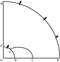
Figure 1: Meridian region of numerical calculation. The region enclosed by a curve $ABLA$ is a corotating region. Plasma is injected through the polar region $PA$ and goes out through the outer radius $QR$. A line $OQ$ is polar axis, and $OR$ is an equator.

2.3 Injection model

In our model, plasma is assumed to flow through a small polar region, $0\leq\theta\leq\theta_{0}$, at the inner boundary $r_{0}$, represented by $PA$ in Fig.1. If the stream lines completely agree with the magnetic dipolar field lines, then the stream function is given by $F_{\pm}\propto\sin^{2}\theta/r$ near the surface $r_{0}$. We assume that the function for each particle type slightly deviates from the dipolar configuration near the polar cap region. In our injection model, the stream function in the range of $0\leq\theta\leq\theta_{0}$ is given by

$$F_{\pm}(r_{0},\theta)=\frac{\lambda\sin^{2}\theta}{r_{0}}\left[1\mp\alpha\left(1-\left(\frac{\sin\theta}{\sin\theta_{0}}\right)^{2}\right)\right],$$ (20)

and the current function $S$ is calculated as

$$S=-\frac{8\pi q\lambda\alpha}{cr_{0}}\sin^{2}\theta\left[1-\left(\frac{\sin\theta}{\sin\theta_{0}}\right)^{2}\right].$$ (21)

The constant $\alpha$ determines the deviation from the dipolar field. The poloidal current completely vanishes in the limit of $\alpha=0$, where the positively charged particles and negatively charged particles move along the common stream lines. The scale factor $\lambda$ is chosen as $4\pi q\lambda\alpha=\mu\Omega$, so that the current function can be written as $S\approx-2\Omega G_{d}/c$ near the polar region, where $G_{d}=\mu\sin^{2}\theta/r$. The current function corresponds to the split-monopole solution near the polar region (Michel, 1973). Our current function $S$ smoothly goes to zero at the edge of polar cap, $\theta=\theta_{0}$. This property is different from that of the force-free and ideal MHD approximations in which the function has a discontinuity (Contopoulos et al., 1999; Ogura & Kojima, 2003; Gruzinov, 2005). That is, there is a current sheet.

The current density as a function of angle is calculated as $j_{r}=-4\mu\Omega\cos\theta[1-2(\sin\theta/\sin\theta_{0})^{2}]/r_{0}^{3}$ at the polar cap. The electric current is negative for $0\leq\sin\theta<\sin\theta_{0}/\sqrt{2}$ and positive for $\sin\theta_{0}/\sqrt{2}<\sin\theta\leq\sin\theta_{0}$. The total current ejected through the polar cap region is zero, since $S(r_{0},\theta_{0})=0$. The positive or negative current flow is produced from the charge-separated plasma, i.e, different number-density distribution between two components in our model. The injection flow at $r_{0}$ is calculated from eq.(20) as

$$n_{\pm}v_{\pm r}=\frac{2\lambda\cos\theta}{r_{0}^{3}}\left[1\mp\alpha\left(1-2\left(\frac{\sin\theta}{\sin\theta_{0}}\right)^{2}\right)\right].$$ (22)

We assume that the flow speed $v_{0}$ is relativistic, $\gamma_{0}=(1-(v_{0}/c)^{2})^{-1/2}\gg 1$, and is independent of $\theta$. This property is assumed to be the same for each particle type. The flow direction through the small polar region $\cos\theta\sim 1$ is almost radial and the velocity is $v_{r}\sim c$, so that the number density at $r_{0}$ is approximately given by

$$n_{\pm}=\frac{2\lambda}{cr_{0}^{3}}\left[1\mp\alpha\left(1-2\left(\frac{\sin\theta}{\sin\theta_{0}}\right)^{2}\right)\right].$$ (23)

The charge density is given by

$$\rho_{e}=-\frac{4q\lambda\alpha}{cr_{0}^{3}}\left[1-2\left(\frac{\sin\theta}{\sin\theta_{0}}\right)^{2}\right]=-\frac{\mu\Omega}{\pi cr_{0}^{3}}\left[1-2\left(\frac{\sin\theta}{\sin\theta_{0}}\right)^{2}\right],$$ (24)

where our choice of parameter $4\pi q\lambda\alpha=\mu\Omega$ is used. The typical value of eq.(24) $\mu\Omega/(\pi cr_{0}^{3})=B_{d}\Omega/(2\pi c)$ is the Goldrich-Julian charge density for the field strength $B_{d}$ of magnetic dipole.

Near the polar cap region, the force-free condition is satisfied, so that the current function $S$ and electric potential $\Psi$ depend on the magnetic flux function $G$. We adopt the following forms, $S_{p}(G_{d})$ and $\Phi_{p}(G_{d})$, as a function of dipolar flux function $G_{d}$ as

$$S_{p}=-\frac{2\Omega G_{d}}{c}(1-bG_{d}),$$ (25)

$$\Phi_{p}=\frac{\Omega G_{d}}{c}+\frac{\Omega}{2bc}\left[1-(bG_{d})^{2}\right],$$ (26)

where $b=r_{0}/(\mu\sin^{2}\theta_{0})$. Equation (25) is reduced to eq.(21) at $r_{0}$, and the Poisson equation is approximately satisfied for $\Phi_{p}$ (26) and the charge density (24). The electric current in the force-free condition is generally given by

$$\vec{j}=c\frac{dS}{dG}\vec{B}+\rho_{e}cR\frac{d\Phi}{dG}\vec{e}_{\phi}.$$ (27)

By the straightforward calculations, it is found that the poloidal components of eq.(27) with the expressions $S_{p}(G_{d})$ and $\Phi_{p}(G_{d})$ are satisfied and toroidal component gives a small value $j_{\phi}\approx\rho_{e}c\times(r_{0}/r_{L})^{5/2}\ll j_{r}\approx\rho_{e}c$. We regard $j_{\phi}=0$ and impose the $\phi$-component of the fluid velocity as

$$v_{+\phi}=\frac{n_{-}+n_{+}}{2n_{+}}R_{0}\Omega,~{}~{}~{}~{}v_{-\phi}=\frac{n_{-}+n_{+}}{2n_{-}}R_{0}\Omega,$$ (28)

where $R_{0}=r_{0}\sin\theta$. For this choice, total angular momentum of plasma flow is $m(n_{-}+n_{+})\gamma_{0}R_{0}^{2}\Omega$ at the inner boundary.

We here summarize the boundary conditions at $r_{0}$. Equation (20) is used for $F_{\pm}$ with $4\pi q\lambda\alpha=\mu\Omega$, and eq.(26) for $\Phi$. Two integrals $J_{\pm}$ and $K_{\pm}$ are calculated at $r_{0}$ as a function of polar angle $\theta$ from eqs.(23),(26),(28), $G_{d}$ and $\gamma_{0}$. The relations $J_{\pm}(F_{\pm})$ and $K_{\pm}(F_{\pm})$ are constructed by eliminating $\theta$ in terms of eq.(20).

3 NUMERICAL RESULTS

We use a finite difference method to solve a set of partial differential equations. The typical grid number in the spherical coordinate $(r,\theta)$ is $300\times 100$ for $0.2\leq r/r_{L}\leq 5$ and $0\leq\theta\leq\pi/2$. The polar cap region at the inner boundary is covered by approximately 30 grid points. We have obtained the same result by changing the grid numbers as $150\times 50$ or $450\times 150$. The convergent factor is $\varepsilon\approx 10^{-2}$, and can not be improved so much by the grid refinement. We demonstrate numerically constructed magnetosphere. Parameters used in the numerical calculation are a deviation parameter $\alpha=0.2$, Lorentz factor $\gamma_{0}=10^{2}$ and $q\mu/(mc^{2}r_{L}^{2})=10$. The last dimensionless parameter is magnetic gyration frequency to angular velocity $\Omega=c/r_{L}$ of a star. Numerical results of the plasma flows and electromagnetic fields depend on a single combination, $\eta=q\mu/(mc^{2}\gamma_{0}r_{L}^{2})$, as far as $\gamma_{0}\gg 1$, since the source terms for eqs.(3),(5) and (18) are scaled by it. Thus $\eta$ is a key parameter to determining the global structure. See Appendix for the details.

Figure 3 shows numerical solution of the magnetic function $G$. We also show that of dipole field $G_{d}=\mu\sin^{2}\theta/r$ for the comparison. The poloidal magnetic field is dipole near the inner radius $r_{0}/r_{L}=0.2$. The field gradually deviates from the dipole, and becomes open outside the light cylinder. The field configuration is eventually radial near outer radius $r_{1}/r_{L}=5$. The numerical result provides the last open field line as $G_{0}\approx 1.15\mu/r_{L}$. The critical value is $G_{0}=1.592\mu/r_{L}$ in magnetosphere fulled with rigidly rotating plasma (Michel, 1973, 1991; Mestel & Pryce, 1992), and $G_{0}=1.36\mu/r_{L}$ (Contopoulos et al., 1999), $G_{0}=1.27\mu/r_{L}$ (Gruzinov, 2005) in a solution with the force-free approximation, and $G_{0}=1.26\mu/r_{L}$ (Komissarov, 2006) in MHD simulation. Our value is smaller than that of other models, but is not so different. The total current is different from that of these models, so that there is no reason why the critical value should agree.

Figure 2: Magnetic flux functions. Solid curves denote the flux surfaces of numerical solution for $Gr_{L}/\mu=$ $0.1,0.2,\cdots,1.4$, and dotted curves those of dipole for $G_{d}r_{L}/\mu=$ $0.2,0.4,\cdots,1.4$ starting from the polar axis.

Figure 3: Stream functions for negatively and positively charged fluids. Solid curves denote the flux surfaces of $F_{-}$, and dotted curves those of $F_{+}$ in intervals of $0.1(\lambda\sin^{2}\theta_{0}/r_{0})$.

Figure 3 shows the results of the stream functions for both species. The global structure of stream lines is almost the same as that of the magnetic field lines shown in Fig.3, although the numerical agreement is not so complete. Thus, flows in meridian plane is almost parallel to the magnetic field lines. A difference between $F_{+}$ and $F_{-}$ at large radius originates from the inner boundary condition at $r_{0}$, where the fraction of negatively charged plasma is slightly larger in polar region $\theta\approx 0$, but smaller for $\theta\approx\theta_{0}$. The property extends to the outer radius. At large radius, the flow becomes is radial and the velocity is still relativistic, so that the number density decreases with the radius, $n_{\pm}\approx|\partial_{\theta}F_{\pm}|/(r^{2}\sin\theta)$ $\propto r^{-2}$. However, the fraction $(n_{+}-n_{-})/(n_{+}+n_{-})$ is still finite, and the charge separation remains. Our numerical model shows that negatively and positively charged regions are separated approximately by a curve with $F_{\pm}\approx 0.5(\lambda\sin^{2}\theta_{0}/r_{0})$.

We show numerical result of the electric potential. The contour of the non-corotating part $\Psi=\Phi-\Omega G/c$ is shown in Fig. 5. There is a peak on the polar axis at $r\approx 0.4r_{L}$. The function $\Psi$ decreases toward the outer boundaries, where $\Psi=0$ is imposed as the boundary condition at outer radius, and on the last open magnetic field. Numerical result shows the maximum value $\Psi=0.85\mu\Omega/(cr_{L})$ at $(r,\theta)=(0.4r_{L},0)$. This value is not small, since the maximum of corotating electric potential is $\Omega G/c\approx 1.15\mu\Omega/(cr_{L})$. Total electric potential $\Phi=\Psi+\Omega G/c$ is shown in Fig. 5. Overall structure is very different from the magnetic flux function $G$ or stream functions $F_{\pm}$ shown in Figs.3-3. The difference is clear at the polar region, whereas the agreement becomes better at high latitude region near the equator. Ideal MHD condition $\vec{B}\cdot\vec{E}=0$ is not assumed in our model. The deviation is very large on the polar axis. This feature is closely related with the boundary conditions. As discussed in section 2, the boundary condition of $\Psi$ is not $E_{r}=0$, but $E_{\theta}=0$ on the axis. This mathematical condition may allow the large value of $\Psi$ on the axis. On the other hand, $\Psi$ almost remains zero near the equatorial region from the boundary condition.

Figure 4: Contour of non-corotating part of electric potential $\Psi=\Phi-\Omega G/c$. Contour levels outwardly decrease in intervals of 0.1$\mu\Omega/(cr_{L})$.

Figure 5: Contour of electric potential $\Phi$. Contour levels upwardly decrease in intervals of 0.1$\mu\Omega/(cr_{L})$.

We discuss a consequence of non-ideal MHD field $\vec{B}\cdot\vec{E}\neq 0$. Figure 7 shows contour of the Lorentz factor of positively charged particles normalized by initial one $\gamma_{0}$. At the injection boundary, $\gamma_{+}$ is fixed as $\gamma_{+}=\gamma_{0}=10^{2}$ for all polar cap angle, but there is a gradual increase toward the outer radius. The increase is remarkable at low $\theta$, but $\gamma_{+}$ is almost constant for the flow along the equator. The increase of $\gamma_{+}$ is determined by the Bernoulli integral as $\Delta\gamma_{+}=-q\Delta\Phi/(mc^{2})$, since $0=\Delta K_{+}=\Delta\gamma_{+}+q\Delta\Phi/(mc^{2})$ along each flow line. Thus, large acceleration of positively charged particles toward the polar region can be understood, since available potential difference $-\Delta\Phi$ is large as inferred from Fig. 5. The change of the Lorentz factor $\gamma_{-}$ of negatively charged particles is opposite in the sign, and is given by $\Delta\gamma_{-}=q\Delta\Phi/(mc^{2})$. They are therefore decelerated toward the polar region.

Figure 6: Increase of Lorentz factor for positively charged particles. Contour levels outwardly increase in intervals of 0.01.

Figure 7: Electromagnetic forces acting on a positively charged particle on a stream line. The electric and magnetic forces are shown by solid and dotted arrows. Three dotted curves denote the stream lines.

Figure 7 demonstrates electromagnetic forces acting on a positively charged particle on the stream lines. Two vectors $q\vec{E}$ and $q(\vec{v}\times\vec{B})/c$ in the meridian plan are shown by arrows. The sum of these two forces causes a net acceleration. It is clear that the vector $\vec{E}$ is not perpendicular to the flow lines, and hence accelerates outwardly. The acceleration mechanism works better for the flow toward the polar region. This is another explanation for the increase of the Lorentz factor $\gamma_{+}$ as shown in Fig. 7. This electric effect is opposite for negatively charged particles, which should be decelerated.

In Fig. 9, we show the current function $S$. The poloidal current flows along a curve with a constant value of $S$. Figure 9 demonstrates a return current. That is, two distinct positions at $r_{0}$ are connected by a curve, say, the curve with $S=-0.3\mu/r_{L}^{2}$. Such a global return current is generally produced due to the inertial term in our model. The integral $J_{\pm}$ in eq.(15) is replaced by $G$ in the limit of $m=0$. The stream function $F_{\pm}$ is constant on a constant magnetic surface $G$, and the current function $S=4\pi q(F_{+}-F_{-})/c$ is also constant. The global structure of $S$ should be the same as that of $G$. Therefore, no loop of $S$ is allowed in the limit of $m=0$, since $G$ is open field outside corotation region. In the context of generalized Ohm’s law, the inertial term is a kind of resistivity. This term causes the dissipation of global current, and return current is produced in our model.

We consider the effect of the current decay on the toroidal magnetic field, which is given by $B_{\phi}=S/R$. Figure 9 shows the global structure. The function is zero at the polar axis, on the last open field line of $G$, and has a maximum at $\theta\approx\theta_{0}/\sqrt{2}$ of the polar cap region. The function decreases outwardly. Ratio to the poloidal component is important since the magnetic field strength both of poloidal and toroidal components decreases with radius. The ratio is small, $|B_{\phi}/B_{p}|\leq(r_{0}/r_{L})^{3/2}/2\approx 0.04$ at the inner boundary. We numerically estimated and found that $|B_{\phi}/B_{p}|\approx 0.5$ at $(r_{L},\pi/4)$, and $|B_{\phi}/B_{p}|\approx 1$ at $(4r_{L},\pi/4)$. Outside the light cylinder, the poloidal magnetic field is monopole-like as shown in Fig. 3, so that $|B_{p}|\propto r^{-2}$. On the other hand, $|B_{\phi}|\propto r^{-1}$ along the stream lines in the limit of $m=0$. The slope of $|B_{\phi}|$ slightly becomes steep due to the inertial term, but is not so steep as $\propto r^{-2}$. In this way, toroidal component of the magnetic field is gradually important with radius, although the resistivity is involved in our model.

Figure 8: Contour of current stream function $S$ in intervals of $0.1\mu/r_{L}^{2}$.

Figure 9: Contour of toroidal magnetic field $B_{\phi}$. Contour levels are outwardly for $-B_{\phi}r_{L}^{3}/\mu=3.2,1.6,0.8,0.4,0.2,0.1,0.05$.

The electromagnetic luminosity through a sphere at $r$ is evaluated by radial component of the Poynting flux as

$$L_{\rm{em}}(r)=2\int_{0}^{\pi/2}\frac{c}{4\pi}(\vec{E}\times\vec{B})_{r}2\pi r^{2}\sin\theta d\theta.$$ (29)

The luminosity of the plasma flow is a sum of both species as

$$L_{\rm{plasma}}(r)=2\int_{0}^{\pi/2}mc^{2}(\gamma_{+}n_{+}v_{+r}+\gamma_{-}n_{-}v_{-r})2\pi r^{2}\sin\theta d\theta.$$ (30)

The energy conversion between two flows is possible through the Joule heating $\vec{j}\cdot\vec{E}$, but the total $L_{\rm{em}}(r)+L_{\rm{plasma}}(r)$ should be conserved. In Table 2, numerical results are shown for different radii. We can check the conservation within a numerical error. The energy flux by plasma flow is always much larger than the electromagnetic one, and the conversion is very small in our model. The magnitude of the luminosities is almost fixed by the injection condition. We analytically evaluate these luminosities at $r_{0}$ using the inner boundary conditions, and find that $L_{\rm{em}}=(\mu\Omega\sin^{2}\theta_{0}/r_{0})^{2}/(3c)$ $\approx 0.4\mu^{2}\Omega^{4}/c^{3}$ and $L_{\rm{plasma}}=$ $8\pi mc^{2}\gamma_{0}\lambda\sin^{2}\theta_{0}/r_{0}$ $=2\mu^{2}\Omega^{3}\sin^{2}\theta_{0}/(\alpha\eta r_{0})$ $\approx 115\mu^{2}\Omega^{4}/c^{3}$, where the numerical values $\alpha=0.2$, $\eta=0.1$ and $\sin^{2}\theta_{0}=1.15\Omega/c$ are used. In order to simulate the Poynting flux dominated case, it is necessary to increase the parameter $\eta$.

Table 2: Luminosity through a sphere with radius $r$.

$r/r_{L}$	$L_{\rm{em}}c^{3}/(\mu^{2}\Omega^{4})$	$L_{\rm{plasma}}c^{3}/(\mu^{2}\Omega^{4})$
1.5	0.18	115.57
2.0	0.20	115.55
2.5	0.21	115.54
3.0	0.22	115.53
3.5	0.23	115.53
4.0	0.23	115.53
4.5	0.23	115.53

4 CONCLUSION

We have numerically constructed a stationary axisymmetric model of magnetosphere with charge separated plasma outflow. The stream lines of pair plasma are determined by electromagnetic forces and inertial term. The massless limit corresponds to the force-free and ideal MHD approximations. The global structures of electromagnetic fields and plasma flows are calculated by taking into account the inertial term. In particular, the non-ideal MHD effects are studied. The electrical acceleration or deceleration region depending on the charge species appears. Poloidal current slightly dissipates. Numerical results depend on a single parameter $\eta=q\mu/(mc^{2}\gamma_{0}r_{L}^{2})$ as far as $\gamma_{0}\gg 1$. The number of our model demonstrated in section 4 is $\eta=0.1$, and is small when applying to the pulsar magnetosphere. Typical number $\eta$ is estimated for electron-positron pair plasma, magnetic field $B_{s}$ at the surface and spin period $P$ as $\eta=$ $10^{4}(B_{s}/10^{12}\rm{G})(P/1\rm{s})^{-2}(\gamma_{0}/10^{2})^{-1}$. Our present model is only applicable to highly relativistic injection ($\gamma_{0}\gg 1$) or weaker magnetic fields ($B_{s}\ll 10^{12}$G). It will be necessary to scale up many orders of magnitude to $\eta\sim 10^{4}$ in order to apply the present method to more realistic cases. We in fact tried scaling up in our numerical calculations, but found that it is not straightforward.

The difficulty and the limitation to smaller value of $\eta$ are closely related with boundary conditions and involved physics, as explained below. The Bernoulli integral (16) should satisfy a constraint $K_{\pm}\mp q\Psi/(mc^{2})=\gamma>1$. In our model, we specify $K_{\pm}$ by the injection condition which is fixed at the inner boundary. During the numerical iterations, the magnitude of the function $\Psi$ becomes very large in a certain region, where the condition $K_{\pm}\mp q\Psi/(mc^{2})>1$ is no longer satisfied. It is easily understood that this easily happens for large value of $\eta=q\mu/(mc^{2}\gamma_{0}r_{L}^{2})$, since the typical scale of $\Psi$ is $\mu/r_{L}^{2}$. This gives a certain upper limit to the choice of $\eta$. The actual estimate of the limit is somewhat complicated, since the potential $\Psi$ depends on the choice of boundary conditions, especially injection model at inner radius. It is therefore necessary to explore consistent boundary conditions or to include some physical process, in order to calculate the models with larger $\eta$. Adjusting mechanism may be required at the boundary or within the numerical domain. For example, our present inner boundary is one-way, i.e, injection only at fixed rate. During numerical iterations, the charge density might numerically blow up elsewhere due to poor boundary condition. If the injection rate is able to be adjusted or plasma is absorbed through the boundary, the increase may be suppressed. However, this is a very difficult back-reaction problem. The boundary conditions are normally used to determine the inner structures. The adjustable boundary conditions should be controlled by the interior. Thus, the boundary conditions and the inner structures should be determined simultaneously. Such numerical scheme is not known and should be developed in future. Otherwise, extensive study to find out consistent boundary conditions for large $\eta$ is required. Our numerical method will be improved by either approach.

Pulsar magnetosphere is described in most spatial region by the force-free and ideal MHD approximations, which correspond to the limit of $\eta\gg 1$. Stationary axisymmetric magnetosphere is constructed so far by a solution of the Grad-Shafranov equation with these approximations (Contopoulos et al., 1999; Ogura & Kojima, 2003; Gruzinov, 2005). Poloidal magnetic field approaches a quasi-spherical wind at infinity. There is a discontinuity in toroidal magnetic field at the boundary of the corotating region, where the current sheet is formed. Lovelace et al. (2006) have obtained an alternative solution of the same equation, but with a different injection current. Their solution exhibits a jet along polar axis and a disk on the equator. There is no current sheet in their numerical model. Thus there are at least two models in the strong magnetic field limit, $\eta\gg 1$. The poloidal magnetic field at infinity is quasi-spherical and there is no current sheet in our numerical solution. It is interesting to examine the model sequence by increasing the parameter $\eta$. Some plasma flow should be highly constrained to a thin region, or the jet-disk system should be formed in the large $\eta$ limit. It is unclear whether or not many solutions exist, depending on physical situations including the plasma state. In order to address these questions, it is necessary to construct the magnetosphere with plasma flow beyond the force-free and ideal MHD approximations. We have here presented a possible approach, although the improvement is needed.

Appendix A DIMENSIONLESS FORMS

We consider the dimensionless forms of eqs. (3),(5) and (18). The magnetic function $G$ is normalized in terms of the magnetic dipole moment $\mu$ and the distance to light cylinder $r_{L}$ as $G=\mu G^{\dagger}/r_{L}$, where a symbol ^† denotes a dimensionless quantity. The electric potential $\Psi$ is expressed as $\Psi=\mu\Omega\Psi^{\dagger}/(cr_{L})$ $=\mu\Psi^{\dagger}/r_{L}^{2}$. Two integrals (15) and (16) are written as $J_{\pm}=\gamma_{0}cr_{L}J^{\dagger}_{\pm}$ and $K_{\pm}=\gamma_{0}K^{\dagger}_{\pm}$, where

$$J^{\dagger}_{\pm}=\left(\frac{\gamma_{\pm}}{\gamma_{0}}\right)\left(\frac{v_{\pm\phi}}{c}\right)\left(\frac{R}{r_{L}}\right)\pm\eta G^{\dagger},$$ (31)

$$K^{\dagger}_{\pm}=\left(\frac{\gamma_{\pm}}{\gamma_{0}}\right)\pm\eta\Psi^{\dagger}.$$ (32)

These values depend on a dimensionless parameter $\eta=q\mu/(mc^{2}\gamma_{0}r_{L}^{2})$. As for the stream function $F_{\pm}$, the normalization constant is $\mu\Omega/(qr_{L})=\mu c/(qr_{L}^{2})$ and $F_{\pm}=\mu\Omega F_{\pm}^{\dagger}/(qr_{L})$. The number density is normalized from eq.(12) as $n_{\pm}=\mu\Omega n_{\pm}^{\dagger}/(qcr_{L}^{3})$. Electric charge and current densities are normalized as $\rho_{e}=\mu\Omega\rho_{e}^{\dagger}/(cr_{L}^{3})$ and $\vec{j}=\mu\Omega\vec{j}^{\dagger}/r_{L}^{3}$ . Using these dimensionless functions, eqs. (3),(5) and (18) can be written as

$${\mathcal{D}}^{\dagger}G^{\dagger}=-4\pi R^{\dagger}j_{\phi}^{\dagger},$$ (33)

$$\left(\nabla^{\dagger}\right)^{2}\Psi^{\dagger}=-4\pi\left(\rho_{e}^{\dagger}-R^{\dagger}j_{\phi}^{\dagger}\right)-2\left(\frac{1}{r^{\dagger}}\right)^{2}\left(r^{\dagger}\frac{\partial}{\partial r^{\dagger}}+\cot\theta\frac{\partial}{\partial\theta}\right)G^{\dagger},$$ (34)

$${\mathcal{D}}^{\dagger}F_{\pm}^{\dagger}=\left[\vec{\nabla}^{\dagger}\ln\left(\frac{n_{\pm}^{\dagger}\gamma_{0}}{\gamma_{\pm}}\right)+\frac{c^{2}\gamma_{0}}{\gamma_{\pm}(v_{\pm r}^{2}+v_{\pm\theta}^{2})}\left(\vec{\nabla}^{\dagger}K_{\pm}^{\dagger}-\frac{v_{\pm\phi}}{cR^{\dagger}}\vec{\nabla}^{\dagger}J_{\pm}^{\dagger}\right)\right]\cdot\vec{\nabla}^{\dagger}F_{\pm}^{\dagger}\pm 4\pi\eta\frac{n_{\pm}^{\dagger}\gamma_{0}}{\gamma_{\pm}}\left(F_{+}^{\dagger}-F_{-}^{\dagger}\right).$$ (35)

where $R^{\dagger}=R/r_{L}$, $r^{\dagger}=r/r_{L}$ and the differential operators with the symbol ^† are defined by $r^{\dagger}=r/r_{L}$. From these expressions, we find that $\eta$ is an important parameter.

References

- Beskin et al. (1993) Beskin, V. S., Gurevich, A. V. & Istomin, Ya. N., 1993, Physics of the Pulsar Magnetospheres, Cambridge University Press
- Contopoulos et al. (1999) Contopoulos, I., Kazanas, D., & Fendt, C., 1999, ApJ, 511, 351
- Goldreich & Julian (1969) Goldreich, P. & Julian, W. H. 1969, ApJ, 157, 869
- Goodwin et al. (2004) Goodwin, S. P., Mestel, J., Mestel, L., & Wright, G. A. E. 2004, MNRAS, 349, 213
- Gruzinov (2005) Gruzinov, A. 2005, Phys. Rev. Lett. 94, 021101
- Gruzinov (2006) Gruzinov, A. 2005, ApJ, 647, L119
- Kalapotharakos & Contopoulos (2008) Kalapotharakos, C. & Contopoulos, I., 2008, arXiv:0811.2863
- Komissarov (2006) Komissarov, S. S., 2006, MNRAS, 367, 19
- Lovelace et al. (2006) Lovelace, R. V. E., Turner, L., & Romanova, M. M., 2006, ApJ, 652, 1494
- McKinney (2006) McKinney, J. C., 2006, MNRAS, 368, L30
- Melatos & Melrose (1996) Melatos, A., & Melrose, D. B., 1996, MNRAS, 279, 1168
- Mestel & Pryce (1992) Mestel, L., & Pryce, M. H. L., 1992, MNRAS, 254, 355
- Mestel & Shibata (1994) Mestel, L., & Shibata, S., 1994, MNRAS, 271, 621
- Mestel (1999) Mestel, L., 1999, Stellar Magnetism, Oxford University Press
- Michel (1973) Michel, F. C., 1973, ApJ, 180, 207
- Michel (1991) Michel, F. C., 1991, Theory of Neutron Star Magnetospheres, University of Chicago Press
- Ogura & Kojima (2003) Ogura, J. & Kojima, Y., 2003, Prog. Theor. Phys., 109, 619
- Spitkovsky (2006) Spitkovsky, A., 2006, ApJ, 648, L51
- Timokhin (2006) Timokhin, A. N. 2006, MNRAS, 368,1055
- Uzdensky (2003) Uzdensky, D. A. 2003, ApJ, 598, 446