Sparse sky grid for the coherent detection of gravitational wave bursts

Abstract

The gravitational wave detectors currently in operation perform the analysis of their scientific data jointly. Concerning the search for bursting sources, coherent data analysis methods have been shown to be more efficient. In the coherent approach, the data collected by the detectors are time-shifted and linearly combined so that the signatures received by each detector add up constructively (thus improving the resulting signal-to-noise ratio). This operation has to be performed over a sky grid (which determines the sky locations to be searched). A limitation of those pipelines is their large computing cost. One of the available degrees of freedom to reduce the cost is the choice of the sky grid. Ideally, the sky sampling scheme should adapt the angular resolution associated with the considered gravitational wave detector network. As the geometry of detector network is not regular (the detectors are not equally spaced and oriented), the angular resolution varies largely depending on the sky location. We propose here a procedure which designs sky grids that permit a complete sky coverage with a minimum number of vertices and thus adapt the local resolution.

1 Introduction

According to Einstein’s theory of General Relativity, the gravitational interaction manifests the geometry of space-time curved by matter. The theory also predicts the existence of radiative solutions to the space-time dynamics which are called gravitational waves. Several detectors (including LIGO in the US, Virgo and GEO in Europe) [1] have been built in the last decade to provide the direct observation of the gravitational waves. They are mainly long-baseline Michelson-type laser interferometers able to sense the weak strain in the arms of the instrument caused by the gravitational waves radiated by astrophysical sources.

While no gravitational wave has been observed so far by these detectors, a first detection is plausible with the sensitivities that will be achieved for the up-coming data takings (labeled S6/VSR2, to start in 2009). Combining gravitational wave data with other types of observations may provide crucial help [2] as they allow better background rejection. For instance, a follow-up search for optical counterparts has been suggested in [3]. The search for coincident high-energy neutrinos has also been proposed in [4].

As these combined searches check the occurence of an (optical or neutrino) event in time/spatial coincidence with the gravitational wave triggers, they rely on an estimate for the location of the gravitational wave source.

Several data analysis pipelines have been proposed to search for bursts of gravitational waves (typically from star collapses or binary mergers), our primary focus here. We will be interested in the ones [5, 6, 7, 8] which perform the coherent processing of the data streams collected by each gravitational wave detectors, as they have shown to be particularly efficient.

In the coherent approach, the data collected by the detectors are time-shifted and linearly combined so that the signatures received by each detector add up constructively if they originate from a given sky location. The transient signal is then searched for in the combined data stream. This operation is repeated by scanning many sky locations. The result is a likelihood sky map which quantifies the “likelihood” of an actual gravitational wave burst source in a particular sky location. The computation of likelihood sky maps requires the discretization of the sky sphere. A uniform sky sampling (see e.g., [9]) is usually used in practice.

A fundamental limitation of the coherent pipelines is their large computational cost. One of the available degrees of freedom to reduce the cost is the choice of the sky grid. On one hand, the computing cost scales linearly with the number of grid points or vertices (the same calculation is repeated for each bin of the sky grid with different data and coherent mixing coefficients). On the other hand, the grid should not be too coarse not to miss any signals. In this paper, we address this trade-off and propose a procedure which designs a sky grid that permits a complete sky coverage with a minimum number of vertices.

This procedure determines the location of the grid vertices on the basis of an estimate of the local angular resolution of the gravitational wave detector network. It thus takes into account both the specific geometry of the detector network and the characteristics of the individual detector antenna patterns. Calibration uncertainties and other timing errors may be also folded in.

We give here a brief outline of the method and connect the various parts to the corresponding section of the paper. In section 2, we describe the context of this study. We describe the characteristics of the signature left by a passing gravitational wave. We spend special attention on the “travel time” (difference in the time of arrival of gravitational waves at each detector with respect to a reference one) and its property because it is an important ingredient for the sky sampling problem.

The direction of a source can be equivalently described in terms of the usual spherical coordinates or using the set of travel times. In section 3, we produce a first sky grid by sampling regularly in the coordinate system associated to the travel times. We propose a robust mapping between the discretized travel times and spherical angles.

The sky grid produced in the first step is “over-sampled” as it is based on timing information only. In a second step presented in section 4, we use the information of the position and orientation of all the detectors and extract the smallest sub-set of vertices that ensures complete sky coverage for a given loss in signal-to-noise ratio. We build this sub-set by casting the grid size minimization as a set covering problem that can be efficiently solved using a greedy procedure based on a dual Lagrangian relaxation heuristic. As an illustration, we produce these sky-grids for an idealized detector network and for the LIGO-Virgo detector network. Section 5 concludes this paper.

2 Framework

Let us consider a network of $D$ gravitational wave detectors. The response of detector $i$ to an incoming gravitational wave emitted from the direction $(\phi,\theta)$ can be written as [8]:

$$s_{i}(t)=\Re\left[F_{i}(\phi,\theta)^{*}h(t-\tau_{i}(\phi,\theta))\right],\hskip 56.9055ptt\geq t_{i}$$ (1)

where $F_{i}$ is the complex-valued antenna pattern ($x^{*}$ denotes the complex conjugate of $x$), and $h(t)=h_{+}(t)+ih_{\times}(t)$ is the complex-valued gravitational wave signal combining the two polarizations $+$ and $\times$. $t_{i}$ is the time of arrival of gravitational wave at detector $i$. In eq. (1), time is defined with respect to a reference which we arbitrarily set to be the time at detector $1$. With this convention, $\tau_{i}(\phi,\theta)=(t_{i}-t_{1})$ denotes the time taken by the wave to travel from detector $1$ to detector $i$. For this reason, we refer to $\tau_{i}(\phi,\theta)$ as travel time. It is proportional to the projected distance between detectors $1$ and $i$ onto the projection direction of the wave, viz.

$$\tau_{i}(\phi,\theta)=\frac{1}{c}(\mathbf{r}_{i}-\mathbf{r}_{1})^{T}\mathbf{w}(\phi,\theta),$$ (2)

where $\mathbf{r}_{i}$ is the coordinate vector of detector $i$, $\mathbf{w}(\phi,\theta)$ is the unit wave vector and $c$ is the speed of light in free space. Here, bold symbols are (column) vectors and $\mathbf{x}^{T}$ denotes the transpose of $\mathbf{x}$.

2.1 Link between spherical coordinates and travel times

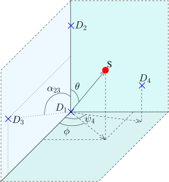
Figure 1: Reference frame — We choose here to work in a reference frame (described for example in [10]) in which expressions linking spherical coordinates and travel times are simple. In this graph, $D_{i}$ corresponds to the position of detector $i$. The origin of the network is chosen to be detector $D_{1}$ which also define our time reference. The $z$ axis is defined as the line joining $D_{1}$ and $D_{2}$. The $x$ axis is defined to be the intersection between the plane orthogonal to the $z$ axis and the plane containing $D_{1}$, $D_{2}$ and $D_{3}$. Finally the $y$ axis is chosen so that the $x$, $y$ and $z$ axes form a right-handed coordinate system. $D_{1}S$ represents the direction of the gravitational wave source.

In this section, we describe the relationship between the spherical coordinates $(\phi,\theta)$ and the set of travel times $\{\tau_{i}(\phi,\theta)\}_{i=1,\dots,D}$. This has already been examined in [10] and this section summarizes some of the results presented in this article.

We choose to work in the reference frame presented in Fig. 1 where the expressions linking spherical coordinates and travel times are simple. Let $T_{i}=d_{1i}/c$ be the time of flight between detectors $D_{1}$ and $D_{i}$ (here $d_{1i}=\|\mathbf{r}_{i}-\mathbf{r}_{1}\|$ is the distance between $D_{1}$ and $D_{i}$). With these notations, the travel time can be expressed with respect to the spherical coordinates $(\phi,\theta)$ in the reference frame by:

$$\tau_{i}=-T_{i}\left(\cos\theta\cos\alpha_{2i}+\sin\alpha_{2i}\cos\left(\phi-\psi_{i}\right)\sin\theta\right),$$ (3)

where $\alpha_{2i}$ is the angle between the lines $(D_{1}D_{2})$ and $(D_{1}D_{i})$ and $\psi_{i}$ is the angle between the $x$ axis and the line $(D_{1}D_{ixy})$ (with $D_{ixy}$ being the projection of $D_{i}$ onto the $xy$ plane).

The spherical coordinates in this frame can be obtained by the reciprocal expressions:

$$\theta =\cos^{-1}\left(-\frac{\tau_{2}}{T_{2}}\right),$$ (4)

$$\phi =\pm\cos^{-1}\left(-\frac{T_{2}\tau_{i}-T_{i}\tau_{2}\cos\alpha_{2i}}{T_{i}\sqrt{T_{2}^{2}-\tau_{2}^{2}}\sin\alpha_{2i}}\right),$$ (5)

with $i\geq 3$. These equations display well-known features of triangulation: the zenith angle $\theta$ can be determined only by two detectors, however the azimuth angle $\phi$ requires at least four detectors to be completely determined (including the sign). Thus alternatively, the set of travel times may be seen as “coordinates” equivalent to the spherical angles.

As we will describe later in Sec. 3, the coordinate system generated by the collection of travel times is more convenient to produce sky grids adapted to the considered detector network. However, this coordinate system is not “standard”. This is why we examine its geometry into some more details now. The 2-sphere is completely characterized by the two spherical angles. For a number $D$ of detectors, the number of travel times is $D-1$. We need to identify the corresponding 2-sphere in the resulting $D-1$- dimensional coordinate space.

From eq. (3), we see that the travel time $\tau_{i}$ takes values in $[-T_{i},T_{i}]$. Therefore, the admissible values for the coordinates $\boldsymbol{\tau}=[\tau_{2},\ldots,\tau_{D}]^{T}$ are located inside a $D-1$-rectangular cuboid. But, for a detector network with $D>2$, the travel time coordinates do not span this cuboid entirely. For instance, it is impossible to have $\tau_{2}=T_{2}$ and $\tau_{3}=T_{3}$ unless $D_{1}$, $D_{2}$ and $D_{3}$ lie on a straight line. From the constraints imposed by the physics, i.e. the propagation of the wave and the geometry of the network, it is possible to determine the admissible surface spanned by the travel time coordinates.

The equation of this two dimensional admissible surface can be obtained from Eq. (3) [10]. It can be written in the form

$$\boldsymbol{\tau}^{T}\mathbf{A}_{D}\boldsymbol{\tau} \leq B_{D}\hskip 56.9055ptD=3\,$$ (6)

$$= B_{D}\hskip 56.9055ptD=4\,.$$ (7)

The expressions of the (symmetric) matrix $\mathbf{A}_{D}$ and $B_{D}$ were obtained in [10] for $D=3$ and $D=4$. We give them below for completeness.

For $D=3$, the admissible surface is an ellipse with

$$\mathbf{A}_{3} =\left[\begin{array}[]{cc}\frac{T_{3}^{2}}{T_{2}^{2}}&-\frac{T_{3}}{T_{2}}\cos\alpha_{23}\\ -\frac{T_{3}}{T_{2}}\cos\alpha_{23}&1\end{array}\right],$$ (10)

$$B_{3} =T_{3}^{2}\sin^{2}\alpha_{23}.$$ (11)

For $D=4$, the admissible surface is an ellipsoid. If $\mathbf{A}_{4}\equiv(A)_{ij}$, we then have

$$A_{11} = \frac{T_{4}^{2}}{T_{2}^{2}}\left[\left(\cos\alpha_{24}-\sin\alpha_{24}\cos\psi_{4}\cot\alpha_{23}\right)^{2}+\left(\frac{\sin\alpha_{24}}{\sin\alpha_{23}}\sin\psi_{4}\right)^{2}\right],$$

$$A_{22} = \left(\frac{T_{4}\sin\alpha_{24}}{T_{3}\sin\alpha_{23}}\right)^{2},$$

$$A_{33} = 1,$$

$$A_{12} = \frac{T_{4}^{2}}{T_{2}T_{3}}\frac{\sin\alpha_{24}}{\sin\alpha_{23}}\left(\cos\alpha_{24}\cos\psi_{4}-\sin\alpha_{24}\cot\alpha_{23}\right),$$

$$A_{13} = -\frac{T_{4}}{T_{2}}\left(\cos\alpha_{24}-\sin\alpha_{24}\cos\psi_{4}\cot\alpha_{23}\right),$$

$$A_{23} = -\frac{T_{4}}{T_{3}}\frac{\sin\alpha_{24}}{\sin\alpha_{23}}\cos\psi_{4},$$

while $B_{4}=T_{4}^{2}\sin^{2}\alpha_{24}\sin^{2}\psi_{4}$.

With the projection of the ellipsoid onto the ($\tau_{i},\tau_{j}$) plane, we retrieve the ellipse for the corresponding $D_{1}$, $D_{i}$ and $D_{j}$ three-detector network. The two points from the two shelves of the ellipsoid which get projected in a single one are associated to the two possible values for $\phi$ in Eq. (5).

For $D>4$ detectors, it is not straightforward to determine the equation of the admissible surface. However, we notice that any triplet taken from the set $\{\tau_{i}(\phi,\theta)\}_{i=2,\dots,D}$ must verify the corresponding ellipsoid equation. The admissible surface is thus the intersection of $C^{D-1}_{3}$ ellipsoidic cylinders. Those equations are redundant. As a sky location is associated to one travel time triplet only, all travel times can be determined from three of them. We need one equation to get one “master” travel time triplet and $D-1-3$ equations to determine the remaining travel times, thus a total of $D-3$ equations.

3 Sampling the travel time space and mapping to sky grid

The coherent analysis follows directly from the computation of the “global” or “network” likelihood ratio testing the presence of a signal in the output from all detectors jointly. The network likelihood ratio involves linear combination of the data streams such that the response of the detectors to an incoming gravitational wave adds coherently. This implies the adjustment of the data streams in time and phase [8, 6, 7]. Time delays are applied to “synchronize” the various responses, i.e. compensate the travel time of the wave between detectors. Clearly, these time delays are intimately related to the travel time coordinates introduced in the previous section.

Following the principle of the generalized likelihood ratio test, in presence of unknown parameters, the network likelihood ratio (more precisely its $-\log$) is maximized over those parameters. Here, the parameters are the coordinates of the source location $\phi$ and $\theta$ and the parameters connected to the physical characteristics of the source (e.g., orientation of the orbital plane for an inspiralling binary, masses of the binary stars) and to the waveform morphology (e.g., central frequency for a sine-Gaussian type bursts).

We are interested here in the maximization over $\phi$ and $\theta$. Mathematically, this is a non-linear optimization problem (due to the adjustment of the time delays in particular). The standard approach for its resolution is to find the maximum of the network likelihood ratio over a sky grid. Instead of the usual scheme based on the uniform discretization of the spherical coordinates, we propose here to discretize (the admissible surface of) the travel time coordinates introduced in the previous section. The resulting sky grid is built using (at least part of) the geometry of the detector network (i.e., the relative position of the detectors) and is thus more adapted to the problem at hand. The procedure goes in two steps. We first present the adequate sampling of the travel times. Then we map the sampled travel times to actual sky locations.

3.1 Sampling the travel time admissible surface

The data streams at the detectors are sampled at a given sampling frequency $f_{s}$. We propose here to sample the travel time coordinates with the same pace. This presents the great advantage that the time delays applied in the coherent analysis are an integer number of samples. No interpolation procedure is thus needed to compute the coherently combined data streams.

In the following, we will label with a superscript $s$ the sampled variables. Let $t_{i}^{s}$ denote the closest time sample from time $t_{i}$ at detector $i$. We have $t_{i}^{s}=t_{i}f_{s}+\epsilon_{i}$ with $\epsilon_{i}\in(-0.5,0.5)$ the truncation error.

The travel time being the time difference $\tau_{i}=t_{i}-t_{1}$, its sampled version $\tau_{i}^{s}=t_{i}^{s}-t_{1}^{s}$ is affected by two truncation errors since $\tau_{i}^{s}=\tau_{i}f_{s}+\epsilon_{i}-\epsilon_{1}$. Now considering the entire set of coordinates defined in Sec. 2.1, we have

$$\boldsymbol{\tau}^{s}=\boldsymbol{\tau}f_{s}+\boldsymbol{\epsilon}-\epsilon_{1}\mathbf{1}$$ (12)

where $\mathbf{1}$ is a vector with all the entries equal to $1$.

For all $\boldsymbol{\tau}$ on the admissible travel time surface, we want to find the integer vectors $\boldsymbol{\tau}^{s}$ provided that $\epsilon_{1}$ and the components of $\boldsymbol{\epsilon}$ are in $(-0.5,0.5)$. Let us first assume that $\epsilon_{1}=0$. We accept $\boldsymbol{\tau}^{s}$ if the admissible surface intersects the cube of edge $1$ centered on $\boldsymbol{\tau}^{s}$. Now, consider that $\epsilon_{1}\neq 0$. We accept $\boldsymbol{\tau}^{s}$ if there exists $\epsilon_{1}\in(-0.5,0.5)$ such that the admissible surface translated by $\epsilon_{1}\mathbf{1}$ intersects the cube of edge $1$ centered on $\boldsymbol{\tau}^{s}$. This method ensures that the boundaries of the admissible surface get well sampled. This precaution is essential for four and more detector case since all points of the admissible surface belong to the boundary.

We demonstrate this method for $D=3,4$ detector network as illustrated in Figure 2. For a three detector network, the admissible surface is an ellipse. Most of the admissible samples lie inside the ellipse for which the proposed method is very efficient. For D=4, the admissible surface is an ellipsoid which makes the admissibility criterion difficult to verify. This is mainly because all of the admissible points lie on the boundary and the criterion amounts to determining the intersection of an ellipsoid and a 3-cube. However we simplify the selection criterion by looking for cubes that have at least one vertex inside the ellipsoid and at least one outside. The result of this simplified method is presented in Figure 2.

For larger detector network, this basic method has to be abandoned since the admissible surface is not known analytically. One possibility is to use Monte Carlo (MC) trials: generate a random set of uniformly distributed sources, compute the wave arrival times and collect the list of distinct discretized travel times. The MC method has the additional advantage that the samples with a very low probability of appearance, i.e. samples with a small intersection between the sample cube and the set of translated admissible surface, are automatically dismissed.

Table 1 gives a comparison of the different discretization methods. As expected, taking the physical properties of travel times (the admissible surface) into account decreases significantly the number of samples. Also the larger the detector network, the more samples are discarded by the MC method. This means that the number of very unlikely samples increases with the number of detectors. Note finally that the proportion of samples being dropped by the MC method increases with the sampling frequency.

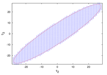
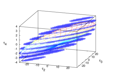
Figure 2: Admissible surfaces of travel times for a three (left, ellipse) and four (right, ellipsoid) detector network and their sampling ($f_{s}=$ 1024 Hz). The unit is milliseconds. The positions of the detectors corresponds to the actual positions of Virgo (Pisa, Italy), LIGO H (Hanford, WA, US) and LIGO L (Livingstone, LA, US) with GEO (Hannover, Germany) added for the four detector case. The sample points obtained with the method described in Sec. 3.1 are indicated with blue dots. Part of the points appear to fall slightly off the admissible surface due to round-off (see discussion in Sec. 3.2).

$f_{s}$ (Hz)		512	1024	2048	4096
A: 3-det	$N_{c}$	841	3,249	12,543	49,275
	$N_{a}$	285	1,002	3,726	14,341
	$N_{MC}$	285	1,001	3,723	14,336
B: 4-det	$N_{c}$	4,205	29,241	188,145	$1.43\times 10^{6}$
	$N_{a}$	869	4,101	22,611	143,155
	$N_{MC}$	866	3,983	16,650	66,454
C: 5-det	$N_{c}$	966,735	$1.35\times 10^{7}$	$1.96\times 10^{8}$	$3.07\times 10^{9}$
	$N_{MC}$	5,725	22,985	90,740	351,171

Table 1: Comparison of various for the discretization schemes used for the travel time space. — $N_{c}$, $N_{a}$ and $N_{MC}$ are the total number of grid points of the travel time grids obtained (i) if their physical properties are ignored (i.e., uniform sampling of $\tau_{i}$ between $[-T_{i},T_{i}]$), (ii) if we sample the admissible surface with the method described in Sec. 3.1, (iii) from the Monte-Carlo search described in Sec. 3.1, resp. The network A is composed of Virgo, LIGO H and LIGO L. The network B is composed of these 3 detectors plus GEO (Hannover, Germany). The network C is composed of these 4 detectors plus a detector located in Japan (assumed to be at the location of the decommissioned detector TAMA.)

3.2 From travel time coordinates to spherical angles

If physically admissible, travel time coordinates can be mapped into spherical coordinates using Eqs. (4) and (5). Some of the travel time samples fall close but outside the admissible surface because of the sampling round-off error (see Fig. 2). While this seems marginal in the 3-detector case (because it happens to the small number of points at the boundary of the admissible ellipse), it is the case for almost all samples in the 4-detector case. A procedure is needed to map points that are slightly off the admissible surface to a sky position. We investigate this question here.

Assuming a given $\boldsymbol{\tau}^{s}$, we search for the closest $\boldsymbol{\tau}$ belonging to the travel time admissible surface $\mathcal{S}$:

$$\boldsymbol{\tau}^{\star}=\arg\min_{\boldsymbol{\tau}\in\mathcal{S}}\|\boldsymbol{\tau}^{s}f_{s}-\boldsymbol{\tau}\|^{2}_{\mathbf{X}}\equiv\mathcal{P}_{\mathcal{S}}(\boldsymbol{\tau}^{s}f_{s}),$$ (13)

where $\|x\|_{\mathbf{X}}$ is the norm associated with the inner product induced by the positive definite matrix $\mathbf{X}$. $\mathcal{P}_{\mathcal{S}}(\cdot)$ is thus the projector onto $\mathcal{S}$ defined by this inner product.

We may opt for a standard least-square minimization by setting $\mathbf{X}$ to identity. In a more accurate version, we may also model the timing errors $\epsilon_{i}$ in Eq. (12) as Gaussian random variables with zero mean and variance $\sigma_{i}^{2}$ and use $\mathbf{X}=\mathrm{diag}[\sigma_{2}^{2},\ldots,\sigma_{D}^{2}]+\sigma^{2}_{1}\mathbf{1}\mathbf{1}^{T}$. In this last case, $\boldsymbol{\tau}^{\star}$ in Eq. (13) is the maximum likelihood estimator of $\boldsymbol{\tau}$ (and associate sky location). The use of this estimator does not restrict to the present sky sampling problem, but it is also useful in the standard triangulation scheme [11] used to obtain the source position from a set of measured arrival times. Note that the model (i.e., the values of $\sigma_{i}$) may be tuned to integrate various timing errors (such as calibration uncertainties).

Let us consider networks with $D=3$ or $4$ detectors. In the case where $\mathbf{X}=\mathbf{I}$ and including the quadratic expression of $\mathcal{S}$ in Eq. (6), we are led to the following constrained minimization problem

$$\min_{\boldsymbol{\tau}}\boldsymbol{\tau}^{T}\boldsymbol{\tau}-2(\boldsymbol{\tau}^{s}f_{s})^{T}\boldsymbol{\tau}\mathrm{~{}~{}subject~{}to~{}~{}}\boldsymbol{\tau}^{T}\mathbf{\mathcal{A}}\boldsymbol{\tau}=1$$ (14)

where $\mathbf{\mathcal{A}}=\mathbf{A}_{D}/B_{D}$. The case with an arbitrary $\mathbf{X}$ can be re-casted into this one by setting $\boldsymbol{\tau}^{\prime}=\mathbf{X}^{1/2}\boldsymbol{\tau}$ and $\mathbf{\mathcal{A}}^{\prime}=(\mathbf{X}^{-1/2})^{T}\mathbf{\mathcal{A}}\mathbf{X}^{1/2}$. This problem can be solved with the method of Lagrange multipliers. It follows that the solution is $\boldsymbol{\tau}=(\mathbf{I}+\lambda\mathbf{\mathcal{A}})^{-1}\boldsymbol{\tau}^{s}f_{s}$ where the Lagrange multiplier $\lambda$ satisfies the polynomial equation:

$$(\boldsymbol{\tau}^{s}f_{s})^{T}(\mathbf{I}+\lambda\mathbf{\mathcal{A}})^{-T}\mathbf{\mathcal{A}}(\mathbf{I}+\lambda\mathbf{\mathcal{A}})^{-1}\boldsymbol{\tau}^{s}f_{s}=1.$$ (15)

This equation can be solved by standard root finding algorithms (in the 3-detector case, Eq. (15) is a fourth-order polynomial that can be solved analytically by radicals with Ferrari’s method).

This methodology has to be adapted for networks with $D\geq 5$ detectors. As discussed in Sec. 2.1, the admissible surface is described by a set of (at most) $D-3$ quadratic equations (each corresponding to the ellipsoid equation for a travel time subset). Consequently, the number of constraints imposed in the minimization problem of Eq. (14) is increased to $D-3$. This problem cannot be solved using the Lagrangian multipliers as before. It can however be viewed as a quadratic programming problem with non-convex quadratic constraints for which numerical methods have been developed [12, 13, 14].

We have applied these mapping algorithms to the travel time grids presented in Fig. 2 with results in Fig. 3 and to a five-detector network with result in Fig. 4. Note that the spherical maps in these figures as well as all the other presented in this article are obtained using a Hammer-Aitoff projection and using as reference frame the geographic coordinate system.

As expected the sampling is not uniform as it depends on the network geometry which is irregular. In particular, the grid gets loose in the vicinity of detector plane ($\phi=0$ in the reference frame in Fig. 1). The 3-detector sky grid appears to be much more structured than the 4-detector one. An explanation of these structures is given in the caption of Fig. 3.

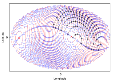
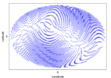
Figure 3: Sky grids associated to the sampling of the admissible travel time surface presented in Fig. 2 obtained by the robust mapping procedures described in Sec. 3.2. The grid obtained for the 3-detector network (left) shows a much more structured distribution than the one obtained for the 4-detector network (right). This structure can be briefly explained as follows: first, the “sinusoidal” line which splits the figure in two halves corresponds to the detector plane ( $\phi=0$ in the network frame, see Fig. 1). The two crosses $\times$ (in red) indicate the points $(\phi,\theta)=(0,0)$ and $(0,\pi)$. The grid results from the intertwinement of several collections of concentric circles: the first set of circles is contours of the polar angle $\theta$ (or equivalently $\tau_{2}$, indicated in red), the second refers to contours of $\tau_{3}$ (semicircles shown with black $+$) and the third set is formed by contours of $\tau_{2}=\tau_{3}+C^{st}$. The two sky points along which the third set is centered correspond to the minimum and maximum values of $C^{st}$. Geometrically, for a special case of VHL where $T_{2}\sim T_{3}$, these 2 sky points correspond to the sky directions along the axis (in the LHV plane) perpendicular to the angle bisector $D_{2}-D_{1}-D_{3}$ (or L-V-H). It mimics the geometry of the sphere with these two points acting as poles and the contour $\tau_{2}=\tau_{3}$ acts like an equator. In any three detector case, this equator is defined by $\phi=0$ and $\theta=\tan^{-1}(T_{2}-T_{3}\cos\alpha_{23})/(T_{3}\sin\alpha_{23})$.

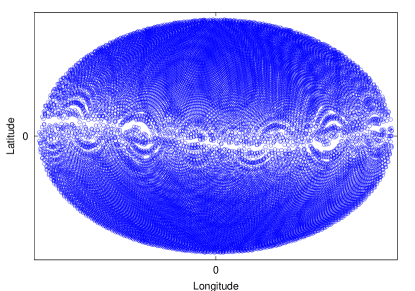
Figure 4: Sky grid associated to the sampling of the admissible surface for the five-detector network C (see Table 1) and assuming $f_{s}=1024$ Hz. Clearly, the sky sampling is much tighter than the one obtained for other networks. This is due to the far location (Japan) of the additional detector. The information given by the time delays between this detector and the others is very accurate and thus valuable.

4 Smallest grid with complete sky coverage

In the previous sections, we have shown how to produce a sky grid from the discretization of the travel time/time delay space. As this grid is built from timing information only, it does not use all the available information (i.e., detector orientation and aperture). The consequence is that this grid is “oversampled”. Its large size generally prevents coherent searches to be performed in real time with current computers. We want to extract from the sky grid the smallest subset ensuring the entire sky coverage. This means that we want that the loss due to the mismatch between any source direction and the closest grid point be not too large. In this section, we describe the selection procedure of the sky grid which tightly covers the sky sphere with the minimal number of grid points. Our procedure results in selecting the grid points in areas of the sky where the position estimation is accurate, and withdrawing samples in areas where the accuracy is poor.

4.1 Angular resolution from the network statistic expansion

Coherent analysis follows directly from the computation of the network likelihood ratio testing the presence of a signal in the output from all detectors jointly. The likelihood ratio is a function $L$ of the data and of the unknown parameters that characterise the expected signal. According to the principle of the generalized likelihood ratio test [15], the network likelihood ratio (its $-\log$, precisely) is maximized over the parameters. We assume here that this maximization has been done for all parameters but the source coordinates $\phi$ and $\theta$, which leads to the likelihood sky map $L(\phi,\theta)$. When a signal is present, it is expected that this function peaks where the source lies. In this section, we investigate the width of the peak.

Let us consider that there is a GW source in the direction $(\phi_{0},\theta_{0})$. We obtain the peak width by the Taylor expansion of $L(\phi,\theta)$ about $(\phi_{0},\theta_{0})$:

$$L(\phi,\theta)\approx L(\phi_{0},\theta_{0})+\frac{1}{2}\sum_{\alpha,\beta}\partial^{2}_{\alpha\beta}L|_{\phi_{0},\theta_{0}}\Delta\alpha\Delta\beta$$

where $\alpha,\beta$ = $\phi$ or $\theta$ in the summation and we have $\Delta\phi=\phi-\phi_{0}$ and $\Delta\theta=\theta-\theta_{0}$.

In the case where the incident wave $h(t)=A(t)\exp i\varphi(t)$ is a quasi-periodic burst of amplitude $A(t)$ and phase $\varphi(t)$, the likelihood ratio is expressed as [5]

$$L(\phi,\theta)=\sum_{n,m=1}^{D}P_{nm}C_{n}C^{*}_{m},$$ (16)

where the correlation measurement is $C_{n}=\int x_{n}(t)\tilde{h}^{*}(t-\tau_{n})dt$, denoting $x_{n}(t)$ the strain data at detector $n$ and $\tilde{h}(t)$ the expected waveform defined above normalized to unit ${\cal L}_{2}$ norm. The operator $\mathbf{P}=(P)_{mn}$ projects onto the vector space generated by the antenna pattern vectors $\mathbf{F}=(F)_{n}$ and $\mathbf{F}^{*}$.

The second derivatives of the likelihood ratio can be calculated following [5] (Sec. V A). The Hessian matrix reads

$$\partial^{2}_{\alpha\beta}L|_{\phi_{0},\theta_{0}}=-\sum_{n,m=1}^{D}\Re\{p_{nm}\}g^{nm}_{\alpha\beta}.$$ (17)

where the weights are $p_{mn}\equiv P_{mn}F_{n}F^{*}_{m}$. The metric components can be calculated explicitly

$$g^{nm}_{\alpha\beta}=\int\!\!\!\int{\cal A}^{2}(t){\cal A}^{2}(s)\partial_{\alpha}(\dot{\varphi}(t)\tau_{n}-\dot{\varphi}(s)\tau_{m})\partial_{\beta}(\dot{\varphi}(s)\tau_{n}-\dot{\varphi}(t)\tau_{m})\>dtds$$ (18)

by invoking slow variations of the amplitude as to compared to the phase’s $\dot{A}/A\ll\dot{\varphi}$ and denoting ${\cal A}(t)$ the signal amplitude after whitening (i.e., division of the spectrum by $\sqrt{S(f)}$ where $S(f)$ designates the PSD of the instrumental noise which we assume identical at all detectors).

If the burst is monochromatic $\varphi(t)=2\pi f_{0}t+\varphi_{0}$ with a constant amplitude $A(t)=1$ (which the case we consider in the simulations presented in the next sections), this simplifies to

$$g^{nm}_{\alpha\beta}={\cal A}_{0}^{2}[\partial_{\alpha}\cdot\partial_{\beta}]\left(2\pi f_{0}(\tau_{n}-\tau_{m})\right),$$ (19)

where ${\cal A}_{0}\propto 1/S(f_{0})$. It is interesting to note that the diagonal terms $g^{nn}_{\alpha\beta}$ are zero so that the Hessian matrix in Eq. (17) vanishes when the projection operator is diagonal. This is true for instance when the number of detectors is $D=2$ as $\mathbf{P}=\mathbf{I}$ in that case (in words, this is equivalent to saying that it is not possible to locate the GW source from two detectors only).

In the case of co-aligned (but not colocated) detectors (with identical antenna patterns $F$), the above expression are further simplified. We realize that this configuration is unrealistic as the detectors are built on a spherical Earth. However, it provides us a case where calculations and simulations are simpler. In this case, $p_{mn}=|F|^{2}/D$

$$\partial^{2}_{\alpha\beta}L|_{\phi_{0},\theta_{0}}=-{\cal A}_{0}^{2}\frac{|F|^{2}}{D}(2\pi f_{0})^{2}\sum_{nm}\partial_{\alpha}(\tau_{n}-\tau_{m})\partial_{\beta}(\tau_{n}-\tau_{m})$$ (20)

With the above Taylor expansion, we can estimate the SNR loss due to a mismatch between the pointing direction and the exact source direction. Let $\mu$ denote the tolerable fraction of amplitude SNR loss. The grid cell is thus defined by

$$\sum_{\alpha,\beta}\partial^{2}_{\alpha\beta}L|_{\phi_{0},\theta_{0}}\Delta\alpha\Delta\beta\leq 2L(\phi_{0},\theta_{0})\left(1-\mu^{2}\right)$$ (21)

with $L(\phi_{0},\theta_{0})={\cal A}^{2}|F|^{2}$.

This equation represents an ellipse centered at $(\phi_{0},\theta_{0})$. The solid angle subtended by the ellipse expresses the angular resolution achievable at this particular sky position. In Fig. 5, we show the (logarithm of the) angular resolution computed for a pure tone. It is useless to sample the celestial sphere with a bin size smaller than this ellipse if the goal is to get a fractional SNR loss of at most $\mu$. Note that while this requirement (with typically $\mu\approx 95\%$) is adequate for detecting a potential source, it is probably not sufficient for estimating its sky position.

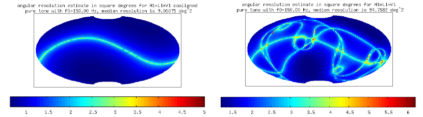
Figure 5: Estimate of the angular resolution given by the ($\log_{10}$) solid angle (in square degrees) subtended by the ellipse defined in Eq. (21) for the 3 detector network A in Table 1 assuming coaligned detectors (left) and real orientation of the detectors (right). The signal is a pure tone of frequency $f_{0}=150$ Hz. In the first case, the angular resolution degrades when the coming wave has a small incidence w.r.t the detector plane (a similar effect appears with the classical triangulation method). The situation is clearly more complicated in the second case: the points where the resolution degrades form complicated patterns resulting from the interplay between the relative positions and orientations of the detectors. Note that the median resolution is about 9 square degrees when the detectors are assumed to be coaligned, while it is 10 times larger, about 94 degrees when considering their true orientation.

4.2 Smallest grid extraction as a covering problem

We want to cover the sky sphere with the smallest number of adjacent sky resolution ellipses. Let $\Omega_{e}=\{s_{k}=(\phi_{k},\theta_{k})\}$ be the sky grid obtained from Sec. 3.2 and let $\mathcal{E}_{k}$ be the set of samples of $\Omega_{e}$ located inside the sky resolution ellipse defined in Eq. (21) associated to $s_{k}$.

We define that two grid points $s_{j}$ and $s_{k}$ are adjacents if $s_{j}\in\mathcal{E}_{k}$ and $s_{k}\in\mathcal{E}_{j}$. Note that the symmetry of this criterion is important as $s_{j}\in\mathcal{E}_{k}$ does not imply that $s_{k}\in\mathcal{E}_{j}$ since the sky resolution ellipses change from points to points.

We search for the smallest subset of samples $\Omega_{s}$ such that all samples in $\Omega_{e}$ are adjacent to at least one sample in $\Omega_{s}$. This problem is similar to the template placement problem encountered for the search of coalescing binaries [16, 17] but there are two major differences. First, an initial sky-grid $\Omega_{e}$ is imposed here. Second, the topology of the parameter space to cover is different: the periodicity of the sphere makes the covering more difficult. In fact, there is no known optimal solution to this problem in the general case. Only an approximated solution can be constructed.

4.3 Solving the covering problem by a greedy procedure

The problem we have at hand can be formulated as an integer optimization problem with linear constraints (see A, Eq. (22)). In this form, it is a particular case of the Set Covering Problem (SCP) [18, 19, 20] which is known to be NP-complete [21]: no polynomial-time algorithm can solve it. Many methods have been proposed (for a survey, see [22]) and we selected the ones of [23] and [24] that can handle large number of variables (typically, the size of $\Omega_{e}$ is $\sim 10^{4}$ to $10^{5}$) and constraints (equal to the square of the initial grid size). We describe the algorithm in details in A. It consists of an efficient greedy procedure based on a dual Lagrangian relaxation of the problem. The greedy procedure iteratively builds a good solution: at each iteration, the variable $x_{k}$ that maximizes a specific cost function is added to the solution and all rows $j$ such that $x_{j}$ and $x_{k}$ are adjacents are removed from the problem, producing a new reduced problem that can be treated in a similar way. In A, we highlight the modifications we made to adapt to the present problem. In particular, we use a cost function based on the information obtained from the sole dual Lagrangian relaxation of the linear problem.

4.4 Application

In this section, we illustrate the method we propose by applying it to two different networks. We consider fictitious networks composed of detectors with parallel orientations. We can check our results against estimates of what should be the grid size in this case. We also consider realistic networks using the actual position and orientation of the main detectors currently in operation.

From Eq. (17), we get the sky resolution ellipses for every samples assuming that the GW has frequency $f_{0}=150$ Hz. This frequency approximately corresponds to the best sensitivity for LIGO and Virgo detectors. We build the corresponding adjacency matrix which feeds the greedy algorithm based on the dual Lagrangian relaxation.

Considering that there are approximately 41,253 square degrees in the whole sphere. From the median angular resolution obtained in Fig. 5, we expect the full sky coverage with a grid of 4500 vertices in the case with coaligned detectors and about 450 vertices considering the true orientation of the detectors.

Detectors with parallel orientations

We first examine the three-detector network A in Table 1 (Virgo, Ligo H and Ligo L, assuming identical noise PSDs and identical orientations) and four detector B (adding GEO). The sampling frequency is set to $f_{s}=4096$ Hz. The size of initial sky grid produced by the procedure in Sec. 3 is $|\Omega_{e}|=28153$. The set covering problem can be qualified as large as the constraint matrix in Eq. (22) is of size $|\Omega_{e}|\times|\Omega_{e}|$. The application of the greedy algorithm based on the dual lagrangian relaxation results in the sky grid presented in Fig. 6 which contains $|\Omega_{s}|=1284$ vertices, i.e. $\simeq 4.6\%$ of the initial number of samples. This result is consistent with that of [5]. Rescaling the results obtained for case III of Table (II) to the special case discussed here, we get a sky grid of size $n_{s}^{\Omega}\sim 1780$ which is comparable to $|\Omega_{s}|$ mentioned above.

This figure also displays a zoom of the resulting grid along with the corresponding ellipses in two small areas. In the area where the ellipse shape and orientation remain roughly constant, we see that the coverage is regularly performed by adjacent ellipses. In area where the ellipses are stretched and have orientation that changes rapidly (this is the case close to the line $\phi=0$ in the detector plane), some degree of overlap is required to have the complete coverage. This case illustrates the importance of the symmetric adjacency proposed and used here.

The minimal sky grid has been computed with various detector networks and various sampling frequencies. The results are tabulated in Table 2. As expected the size of the minimum grid remains more or less constant with the sampling frequency, as it is prescribed by the angular resolution achievable by the detector network.

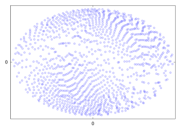
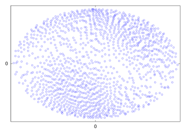
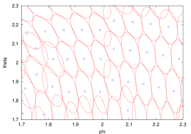
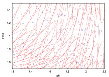
Figure 6: Minimal sky grids for the 3 detector network A (top left, see Table 1 for the description of the networks) and 4 detector network B (top right) assuming parallel orientations (sampling frequency $f_{s}=4096$ Hz) and signal frequency $f_{0}=150$ Hz. The number of vertices in the grid is $1284$ in the first case and $1354$ in the second. Bottom row, we present two blow-up for the 3 detector case: (left) where the sky resolution ellipses have constant size and remain aligned and the other; (right) where the ellipses are strechted and vary rapidly from samples to samples.

$f_{s}$ (Hz)		1024	2048	4096
A: 3-det	exh. set ($|\Omega_{e}|$)	1,868	7,184	28,153
	min. set ($|\Omega_{s}|$)	1,774	1,127	1,284
	$|\Omega_{s}|/|\Omega_{e}|$ ($\%$)	95.0	15.7	4.6
B: 4-det	exh. set ($|\Omega_{e}|$)	3,983	16,650	66,454
	min. set ($|\Omega_{s}|$)	1,454	1,180	1,354
	$|\Omega_{s}|/|\Omega_{e}|$ ($\%$)	36.5	7.1	2.0
C: 5-det	exh. set ($|\Omega_{e}|$)	22,985	90,740	351,171
	min. set ($|\Omega_{s}|$)	2,695	2,979	3,368
	$|\Omega_{s}|/|\Omega_{e}|$ ($\%$)	11.7	3.3	0.96

Table 2: Comparison between the sizes of initial sky grid $\Omega_{e}$ and minimum sky grid $\Omega_{s}$ assuming a parallel orientation for the detectors. We get a typical size of few thousands of vertices which is consistent with the rough estimate drawn from the median resolution in Fig. 5.

To check that good detection performance can still be achieved with the minimum grid, we also compared the performance in terms of false alarm and detection probabilities of both the initial grid and the minimum grid. False alarm and detection rates were evaluated by Monte Carlo method using noise only (using simulated white Gaussian noise) and signal+noise trials. A monochromatic signal with frequency $f_{0}=150$ Hz was injected in the 3-detector network A using a sampling frequency $f_{s}=4096$ Hz. The position of the source was uniformly drawn over the sky sphere. The other signal parameters such as polarization or amplitude were also randomly chosen.

We used the (-log) likelihood ratio introduced in Sec. 4.1 as the detection statistics following the implementation given in [8]. This corresponds to applying a matched filter filtering procedure which results in a likelihood sky map. The maximum of this likelihood map was compared to a threshold to decide for the detection of the GW.

These simulations were repeated for different thresholds. For threshold values, $10^{4}$ Monte Carlo simulations were run. The result obtained is presented in Fig. 7. We observe that the performances obtained with the minimal sky grid are comparable to that of the (“oversampled”) initial sky grid.

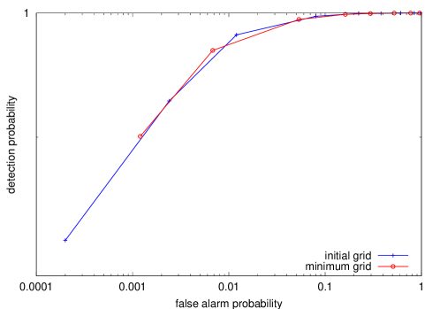
Figure 7: Detection performance in terms of false alarm and detection probabilities for the 3-detector network A (sampling frequency $f_{s}=4096$).

Detectors with their true orientations

Now, we consider the detectors with their true orientation. We show in Fig. 8 the result we get for the four-detector network B in Table 1. The size of the minimum grids are gathered in Table 3 for various configurations.

The resulting grids contain less samples than in the previous case (parallel detectors) due to the additional loss of accuracy which arises when the detectors don’t share the same orientation.

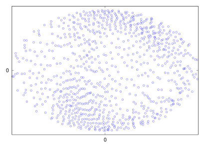
Figure 8: Minimal sky grid ($887$ vertices) for the 4 detector network B (see Table 1) Virgo, Ligo H, Ligo L and GEO with their actual orientation (sampling frequency $f_{s}=4096$ Hz and signal frequency $f_{0}=150$ Hz.)

$f_{s}$ (Hz)		1024	2048	4096
A: 3-det	exh. set ($|\Omega_{e}|$)	1,868	7,184	28,153
	min. set ($|\Omega_{s}|$)	429	391	440
	$|\Omega_{s}|/|\Omega_{e}|$ (in $\%$)	23.0	5.4	1.6
B: 4-det	exh. set ($|\Omega_{e}|$)	3,983	16,650	66,454
	min. set ($|\Omega_{s}|$)	937	817	887
	$|\Omega_{s}|/|\Omega_{e}|$ ($\%$)	23.5	4.9	1.3
C: 5-det	exh. set ($|\Omega_{e}|$)	22,985	90,740	351,171
	min. set ($|\Omega_{s}|$)	1,587	1,723	1,898
	$|\Omega_{s}|/|\Omega_{e}|$ ($\%$)	6.9	1.9	0.54

Table 3: Comparison between the sizes of initial sky grid $\Omega_{e}$ and minimum sky grid $\Omega_{s}$ considering the actual orientation of the detectors. We get a typical grid size of few hundrends of vertices which is consistent with the estimate drawn from the median resolution in Fig. 5.

5 Conclusions

Most coherent detection scheme includes an algorithmic loop over source directions taken from a predefined sky grid. This part of the detection algorithm takes a significant amount of computing ressources. One of the available degrees of freedom to address this issue is the way the sky sphere is sampled. We investigated the possibility to build an optimally “sparse” sky grid which performs the complete sky coverage with the smallest number of vertices. It is clear that the optimal sky grid should adapt the pointing accuracy.

Contrarily to electromagnetic antenna arrays (e.g., used for RADAR applications), gravitational wave detector networks are not arrays of regularly spaced and oriented sensors. The pointing accuracy we get with such network results from the complicated interplay between the relative positions and orientations of the detectors. Because of the network heterogeneity, the pointing accuracy varies largely over the whole sky. In this paper, we build sky grids from an estimate of the “local” angular resolution. The vertex density is reduced where the resolution is coarse and vice-versa.

The method goes into two steps. We first produce a grid from pre-selected sky directions where the travel time between detectors and the time reference is (close to) an integer number of time samples. Those points are convenient because the time-shifts necessary to align in time the signals (i.e., compensate the travel time between the detector and the time reference) received by each detector are trivially performed. This operation amounts to sampling the manifold described by the travel times. This sampling can be determined analytically in the case of three (i.e., the manifold is an ellipse interior) and four detectors (i.e., the manifold is the surface of an ellipsoid). For larger networks, we suggest to apply Monte Carlo procedures. Once done, a key point is to map from travel times to sky directions. To perform this mapping, we propose a method that is robust to the round-off error due to the truncation of the travel times.

In the second step, we extract from the first grid the smallest sub-set of vertices that ensures complete sky coverage for a given loss in signal-to-noise ratio. We build this sub-set by casting the grid size minimization into a set covering problem. The procedure we propose to solve the corresponding linear program with linear and integer constraints relies on a greedy algorithm and a dual Lagrangian relaxation. The resulting grid show considerable reduction in size. We have checked that the results we get with this grid are comparable to what we get when using more resolved sky grids (i.e., at a given false alarm rate, the detection probability are comparable when performing an all-sky blind search). Our investigations have been limited to source detection. It is likely that the sky grid has to be refined if the goal is the accurate determination of the source position.

The overall procedure to build the grid can be quite computationally heavy. However this procedure needs to be done only once beforehand.

Acknowlegments

This research was supported by the Virgo-EGO Scientific Forum.

Appendix A Solving the set covering problem

We propose to formulate the problem of building the minimum sample set as an integer optimization problem with linear constraints in the following way:

$$\begin{array}[]{rl}\min&\displaystyle{\mathbf{u}^{T}\mathbf{x}=\sum_{k=1}^{|\Omega_{e}|}x_{k}}\\ \mathrm{s.t.}&\mathbf{Ax}\geq\mathbf{u},\\ &x_{k}\in\{0,1\},~{}k=1,\dots,|\Omega_{e}|.\end{array}$$ (22)

Here the vector $\mathbf{x}$ of size $|\Omega_{e}|$ is the output vector that should define the minimal set: its entry $x_{k}$ takes value $1$ if the corresponding sample $s_{k}$ is included in $\Omega_{s}$, and $0$ otherwise. Hence, the non-zero entries of $\mathbf{x}$ define the subset $\Omega_{s}$, and the objective function of this optimization problem is the number of samples in the final set (the number of non-zero values of vector $\mathbf{x}$, to be minimized). The vector $\mathbf{u}$ is a column vector of size $|\Omega_{e}|$ such that $\mathbf{u}=[1,\dots,1]^{T}$. Finally the matrix $\mathbf{A}$ of size $(|\Omega_{e}|\times|\Omega_{e}|)$ represents the neighbouring relationships: it is such that $a_{ij}=1$ if $s_{i}$ and $s_{j}$ are neighboors and $a_{ij}=0$ otherwise. Each row $j$ of matrix $\mathbf{A}$ represent a specific constraint on sample $s_{j}$ in the oversampled set: it is here to insure that $s_{j}$ is be adjacent to at least one non zero entry of $\mathbf{x}$, and therefore covered by at least one resolution cell.

As the matrix of linear constraints $\mathbf{A}$ may contain several tens or hundreds of thousands of columns and the same amount of rows (see the number of samples from Table 1, the problem is very difficult and cannot be solved by optimal methods. We therefore propose to use here a method inspired by [23] and [24]. It follows an efficient greedy procedure based on a dual Lagrangian relaxation of the problem. The greedy procedure iteratively builds a good solution in the same way as in [24]: at each iteration, the variable $x_{k}$ that maximizes a specific cost function is added to the solution and all rows $j$ such that $x_{j}\in\mathcal{E}_{k}$ are removed from the problem (because the corresponding constraints are fulfilled by the solution), producing a reduced problem that can be treated in a similar way. Here the cost function is computed thanks to the information obtained from the dual Lagrangian relaxation of the reduced problem. Contrary to the method proposed in [24], we do not use the primal relaxation of (22), which reduces the computational cost of the algorithm as well as the dependency of the method over tunable parameters, and leads to smaller running time and slightly better solutions.

The dual problem of (22) is defined as:

$$\begin{array}[]{rl}\max&\mathbf{u}_{m}^{T}\mathbf{y}\\ \mathrm{s.t.}&\mathbf{A}^{T}\mathbf{y}\leq\mathbf{u}_{n},\\ &y_{k}\geq 0,~{}k=1,\dots,|\Omega_{e}|.\end{array}$$ (23)

The Lagrangian relaxation of the dual problem (23) is given here by:

$$\begin{array}[]{rl}\displaystyle{\min_{\boldsymbol{\mu}}}&\displaystyle{\max_{\mathbf{y}}L(\mathbf{y},\boldsymbol{\mu})}\\ \mathrm{s.t.}&\mu_{i}\geq 0,~{}i=1,\dots,m,\\ &0\leq y_{k}\leq 1,~{}k=1,\dots,n,\end{array}$$ (24)

where $\boldsymbol{\mu}$ is the vector of Lagrange multipliers and $L(\mathbf{y},\boldsymbol{\mu})=\mathbf{u}_{m}^{T}\mathbf{y}-\mu^{T}(\mathbf{A}^{T}\mathbf{y}-\mathbf{u}_{n})$ is the Lagrange function of the dual problem. Here the maximization of $L(\mathbf{y},\boldsymbol{\mu})$ over $y_{k}\in\{0,1\},~{}k=1,\dots,n$ is straightforward: indeed it is obtained by setting $y_{k}=1$ if the $k^{\mathrm{th}}$ column of the row vector $\mathbf{u}_{m}^{T}-\mu^{T}\mathbf{A}^{T}$ is positive, and $y_{k}=0$ otherwise. Besides the function $\max_{\mathbf{y}}L(\mathbf{y},\boldsymbol{\mu})$ is convex in $\boldsymbol{\mu}$, and therefore it can be minimized efficiently by means of a subgradient algorithm. Two main problems arise:

• the optimal values of (23) and of its Lagrangian relaxation (24) may not be equal (duality gap);

• the vector $\mathbf{y}^{*}(\boldsymbol{\mu})$ minimizing $L(\mathbf{y},\boldsymbol{\mu})$ is generally not feasible, i.e. it doesn’t verify the linear constraints $\mathbf{A}^{T}\mathbf{y}^{*}(\boldsymbol{\mu})\leq\mathbf{u}_{n}$.

However, despite these problems, and contrary to the multipliers obtained from the primal Lagrangian relaxation [23], the dual Lagrange multipliers $\boldsymbol{\mu}$ carry very useful information about problem (22). In particular $\boldsymbol{\mu}$ is a near-optimal and near-feasible solution of the linear relaxation of (22). It can therefore be used to decide which variable should be added to the final solution. Here the variable chosen is simply the one corresponding to the largest entry of $\boldsymbol{\mu}$. It should be also noted that all samples $s_{k}$ such that $\mathcal{E}_{k}=\{s_{k}\}$ must be in the final solution set since these points have no adjacent point.

The final greedy algorithm can be summarized as follows:

1. Find the oversampled set $\Omega_{e}$;

2. Build the adjacency matrix $A$;

3. Set the solution set $\Omega_{s}=\emptyset$;

4. Find all points $s_{k}$ such that $\mathcal{E}_{k}=\{s_{k}\}$, add them to $\Omega_{s}$, remove them from the set $\Omega_{e}$ and remove the corresponding rows and columns from the matrix $\mathbf{A}$;

5. While $\Omega_{e}\not=\emptyset$:

   • Solve the dual Lagrangian relaxation (24) of problem (22);

   • Find the largest Lagrange multiplier $\mu_{k}$, add the corresponding sample $s_{k}$ to $\Omega_{s}$, remove the corresponding column from matrix $\mathbf{A}$ as well as all rows $j$ such that $s_{j}$ and $s_{k}$ are neighboors, and reduce the set $\Omega_{e}$ similarly.

It is also sometimes possible to improve the quality of the solution by introducing a randomized criterion for the variable selection. In [24], it was proposed to run several time the algorithm. For the first run, the variable selected is, as described above, the one corresponding to the largest entry of $\boldsymbol{\mu}$. However for the other runs, the variable selected may be the one corresponding to the second largest entry of $\boldsymbol{\mu}$ with probability $0.5$. We adopted this strategy since the choice of the minimum sample set has to be done only once in our case and therefore the additional computational cost induced by running several time the same algorithm is not prohibitive.

References

References

- [1] GEO600 www.geo600.uni-hannover.de, LIGO http://www.ligo.org, Virgo http://www.virgo.infn.it.
- [2] LIGO Scientific Collaboration and Virgo Collaboration. Astrophysically triggered searches for gravitational waves: Status and prospects. Class. Quant. Grav., 25:114051, 2008.
- [3] J. Kanner et al. LOOC UP: locating and observing optical counterparts to gravitational wave bursts. Class. Quantum Grav., 25:184034, 2008.
- [4] Yoichi Aso et al. Search method for coincident events from LIGO and IceCube detectors. Class. Quant. Grav., 25:114039, 2008.
- [5] A. Pai, S. Dhurandhar, and S. Bose. A data-analysis strategy for detecting gravitational-wave signals from inspiraling compact binaries with a network of laser-interferometric detectors. Phys. Rev., D64:042004, 2001.
- [6] S. Klimenko, I. Yakushin, A. Mercer, and G. Mitselmakher. Coherent method for detection of gravitational wave bursts. 2008.
- [7] Shourov Chatterji et al. Coherent network analysis technique for discriminating gravitational-wave bursts from instrumental noise. Phys. Rev., D74:082005, 2006.
- [8] A. Pai, E. Chassande-Mottin, and O. Rabaste. Best network chirplet-chain: Near-optimal coherent detection of unmodeled gravitational wave chirps with a network of detectors. Phys. Rev., D77:062005, 2008.
- [9] N. Arnaud et al. Coincidence and coherent data analysis methods for gravitational wave bursts in a network of interferometric detectors. Phys. Rev., D68:102001, 2003.
- [10] B. Bhawal and S.V. Dhurandhar. Coincidence detection of broadband signals by networks of the planned interferometric gravitational wave detectors. Technical report 29/95, IUCAA, 1995.
- [11] J. Markowitz, M. Zanolin, L. Cadonati, and E. Katsavounidis. Gravitational wave burst source direction estimation using time and amplitude information. 2008.
- [12] K. Anstreicher and H. Wolkowicz. On lagrangian relaxations of quadratic matrix constraints. SIAM J. on Matrix Analysis and Applications, 22(1):44–55, 2000.
- [13] J.B. Lasserre. Global optimization with polynomials and the problem of moments. SIAM J. Optim, 11(3):796–817, 2001.
- [14] D. Henrion and J.B. Lasserre. Gloptipoly: Global optimization over polynomials with matlab and SeDuMi. ACM. Trans. Math. Soft., 29:165–194, 2003.
- [15] H.V. Poor. An Introduction to Signal Detection and Estimation. Springer-Verlag, 1988.
- [16] N. Arnaud et al. Elliptical tiling method to generate a 2-dimensional set of templates for gravitational wave search. Phys. Rev., D67(102003), 2003.
- [17] F. Beauville et al. Variable placement of templates technique in a 2D parameter space for binary inspiral searches. Class. Quantum Grav., 22:4285–4309, 2005.
- [18] N. Christofides and S. Korman. A computational survey of methods for the set covering problem. Management Science, 21(5):591–599, 1975.
- [19] E.K. Baker. Efficient heuristic algorithms for the weighted set covering problem. Computers and Operations Research, 8(6):303–310, 1981.
- [20] J.E. Beasley. An algorithm for set covering problems. European Journal of Operational Research, 31:85–93, 1987.
- [21] R.M. Karp. Reducibility among combinatorial problems. In R.E. Miller and J.W. Thatcher, editors, Complexity of Computer Computations, pages 85–103. Plenum Press, New York, 1972.
- [22] A. Caprara, P. Toth, and M. Fischetti. Algorithms for the set covering problem. Annals of Operations Research, 98:353–371, 2000.
- [23] J.E. Beasley. A lagrangian heuristic for set-covering problems. Naval Research Logistics, 37:151–164, 1990.
- [24] S. Ceria, P. Nobili, and A. Sassano. A lagrangian-based heuristic of large-scale set covering problems. Mathematical Programming, 81(2):215–228, 1998.