Improved Approximation Algorithms for Segment Minimization in Intensity Modulated Radiation Therapy

Abstract

The segment minimization problem consists of finding the smallest set of integer matrices that sum to a given intensity matrix, such that each summand has only one non-zero value, and the non-zeroes in each row are consecutive. This has direct applications in intensity-modulated radiation therapy, an effective form of cancer treatment. We develop three approximation algorithms for matrices with arbitrarily many rows. Our first two algorithms improve the approximation factor from the previous best of $1+\log_{2}h$ to (roughly) $3/2\cdot(1+\log_{3}h)$ and $11/6\cdot(1+\log_{4}{h})$, respectively, where $h$ is the largest entry in the intensity matrix. We illustrate the limitations of the specific approach used to obtain these two algorithms by proving a lower bound of $\frac{(2b-2)}{b}\cdot\log_{b}{h}+\frac{1}{b}$ on the approximation guarantee. Our third algorithm improves the approximation factor from $2\cdot(\log D+1)$ to $24/13\cdot(\log D+1)$, where $D$ is (roughly) the largest difference between consecutive elements of a row of the intensity matrix. Finally, experimentation with these algorithms shows that they perform well with respect to the optimum and outperform other approximation algorithms on 77% of the 122 test cases we consider, which include both real world and synthetic data.

1 Introduction

Intensity-modulated radiation therapy (IMRT) is an effective form of cancer treatment in which the region to be treated is discretized into a grid and a treatment plan specifies the amount of radiation to be delivered to the area of body surface corresponding to each grid cell. A device called a multileaf collimator (MLC) is used to administer the treatment plan in a series of steps. In each step, two banks of metal leaves in the MLC are positioned to cover certain portions of the body surface, while leaving others exposed, and the latter are then subjected to a specific amount of radiation.

A treatment plan can be represented as an $m\times n$ intensity matrix $T$ of non-negative integer values, whose entries represent the amount of radiation to be delivered to the corresponding grid cells. The leaves of the MLC can be seen as partially covering rows of $T$; for each row $i$ of $T$ there are two leaves, one of which may slide inwards from the left to cover the elements in columns $1..l$ of that row, while the other may slide inwards from the right to cover the elements in columns $r..n$. After each step of the treatment, the amount of radiation applied in that step (this can differ per step) is subtracted from each entry of $T$ that has not been covered. The treatment is completed when all entries of $T$ have reached $0$.

Setting leaf positions in each step of the treatment plan requires time. Minimizing the number of steps reduces treatment time and can result in increased patient throughput, reduced machine wear and tear, and overall reduced cost of the procedure. Minimizing the number of steps for a given treatment plan is the objective of this paper.

Formally, a segment is a matrix $S$ such that non-zeroes in each row of $S$ are consecutive, and all non-zero entries of $S$ are the same integer, which we call the segment-value. A segmentation of $T$ is a set of segment matrices that sum to $T$, and we call the cardinality of such a set the size of that segmentation. The segmentation problem is, given an intensity matrix $T$, to find a minimum-size segmentation of $T$. We will often consider the special case of a matrix $T$ with one row, which we call the single-row segmentation problem as opposed to the full-matrix segmentation problem.

The segmentation problem is known to be NP-complete in the strong sense, even for a single row [3, 4, 10], as well as APX-complete [5]. A number of heuristics are known [1, 4, 13, 15, 19, 21]. Approaches for obtaining optimal (exact) solutions also exist [2, 8, 16, 20]; of course, these approaches do not necessarily terminate in polynomial time in the size of the input. Bansal et al. [5] provide a $24/13$-approximation algorithm for the single-row problem and give some better approximations for more constrained versions. Collins et al. [12] show that the single column version of the problem is NP-complete and provides some non-trivial lower bounds given certain constraints. Work by Luan et al. [18] gives two approximation algorithms for the full $m\times{}n$ problem where the approximation factor depends on other parameters of the problem, e.g. the largest entry $h$ in the target matrix. They do not consider the performance of their algorithms in practice. More recent work by [16] has shown that the $m\times{}n$ case can be solved optimally with time complexity $O(m\cdot{}n^{2h+2})$; this approach is shown to computationally intensive even for small $h$ in practice.

Our Contributions

Luan et al. [18] used two properties to obtain approximation algorithms. First, the segmentation problem is straightforward when $h=1$ (0/1-matrices). Second, segmentations for the single-row problem with small segment-values can be used to obtain good segmentations for the full-matrix problem. By exploiting these two properties, Luan et al. obtained two algorithms with respective approximation factors of $1+\log_{2}h$ and $2(1+\log_{2}D)$ where $h$ is the largest value in $T$, and $D$ is roughly the largest difference between consecutive elements in a row of $T$.

In this paper, we extend the ideas of Luan et al. In particular, we prove that the segmentation problem can be approximated when $h=2$ and $h=3$; this is far less straightforward than the case $h=1$. This yields two fast algorithms for the full-matrix segmentation problem with approximation factors (roughly) $\frac{3}{2}\cdot(1+\log_{3}{h})$ and $\frac{11}{6}\cdot{}(1+\log_{4}{h})$, respectively, both of which are less than $1+\log h$. While we show that the general two-stage approach of Luan et al. [18] can be extended to provide superior approximation algorithms, we also prove a limitation of this approach.

We also provide a new approximation algorithm with approximation factor (roughly) $\alpha\log D$, where $\alpha$ is the best approximation factor for the single-row problem. The current best known $\alpha$ is $\alpha=24/13$ [5]; any improved approximation result for the single-row problem would directly lead to an improved approximation result for the full problem. This second approximation algorithm expands on the second approximation algorithm by Luan et al.; they used one specific 2-approximation algorithm for the single-row problem, whereas we show that in fact any $\alpha$-approximation algorithm can be used.

Finally, we give an empirical evaluation of known approximation algorithms for the full $m\times{}n$ segmentation problem, using both synthetic and real-world clinical data. Our experiments demonstrate that the constant factor improvements made by our algorithms yield significant performance gains in practice. Therefore, in both the $O(\log{h})$ and $O(\log{D})$ scenarios, our new algorithms improve on previous approximation algorithms theoretically and experimentally.

2 Improved Approximation Algorithms

A vital insight for our approximation algorithm is the concept of a marker ([18]; this was called tick in [5].) A marker in row $i$ of the target matrix $T$ is an index where the entry of $T$ changes while going along the row. Formally, it is an index $j$ for which $T[i,j-1]\neq T[i,j]$, or $j=1$ and $T[i,1]\neq 0$, or $j=n+1$ and $T[i,n]\neq 0$.

Let $\rho^{i}$ denote the number of markers in row $i$ of $T$, and define $\rho=\max\limits_{\mbox{\tiny{All rows $i$ in $T$}}}\{\rho^{i}\}$, i.e. the number of markers in the row of $T$ which has the most markers over all rows. We begin by restating the following observation noted by Luan et al. that we will later find useful.

Observation 1.

(Luan et al. [18]) Let $OPT$ be the size of a minimal segmentation of an intensity matrix $T$. Then $\rho\leq{}2\cdot{}OPT$.

The first approximation algorithm given by Luan et al. [18] works as follows. Split the given intensity matrix $T$ into matrices $P_{0},\dots,P_{k}$ such that $T=\sum_{\ell=0}^{k}2^{\ell}\cdot P_{\ell}$ (by taking the bits of the base-2 representation of entries of $T$) where $k=\log_{2}{h}$ and each $P_{\ell}$ is a $0/1$-matrix. A segmentation for $T$ can then be obtained by taking segmentations of each $P_{\ell}$, multiplying their values by $2^{\ell}$, and taking their union. Since each $P_{\ell}$ is a 0/1-matrix, an optimal segmentation of it can be found easily, and an approximation bound of $1+\log h$ can be shown.

We use a similar approach, but change the base $b$, writing $T=\sum_{\ell=0}^{k}b^{\ell}\cdot P_{\ell}$ for some integer $b\geq 3$. This raises nontrivial question: How can we solve the segmentation problem in a matrix that has values in $\{0,1,\dots,b-1\}$? And is the resulting segmentation a good approximation of the optimal segmentation?

Assume that we have $\alpha$-approximate segmentations for each $P_{\ell}$, i.e., for each $\ell$ we have a segmentation ${\mathcal{S}}_{\ell}$ of $P_{\ell}$ that is within a factor $\alpha$ of the optimum for $P_{\ell}$, for some $\alpha\geq 1$. We combine these segmentations as follows: For each segment $S$ of ${\mathcal{S}}_{\ell}$, add $b^{\ell}\cdot S$ to ${\mathcal{S}}$. One easily verifies that ${\mathcal{S}}$ is a segmentation of $T$. But it is not obvious that this is a good approximation of the optimum segmentation of $T$. One might think that it is an $\alpha(\log_{b}(h)+1)$-approximation of the optimal segmentation of $T$, but this is not true in general; see also Section 2.3.

It is also not clear how to find a segmentation of $P_{\ell}$ that is good. As mentioned earlier, the optimal segmentation can be found in polynomial time if $b$ is a constant [16], but the running time is not practical, and it is not clear whether it yields a good approximation. Our main contribution is that an approximation guarantee can be established for $b=3,4$. Moreover, it suffices to use a segmentation of $P_{\ell}$ that is not necessarily optimal, but can be found in linear time.

More specifically, we show how to find a segmention of one row of $P_{\ell}$ that can be bound in size depending on the number of markers $\rho$. Moreover, the segmentations of each row can be combined easily into one segmentation of $P_{\ell}$, and the segmentations of all the $P_{\ell}$’s can be combined into a segmentation of $T$, while carrying the bound in terms of $\rho$ along. By Observation 1, this will allow us to bound the size of resulting segmentation relative to the optimum.

We briefly give here the simple algorithm GreedyRowPacking that we use to combine segmentations of rows of a target-matrix $P_{\ell}$ (with values in $1,\dots,b-1$) into a segmentation of the whole matrix $P_{\ell}$. Check for each value $v\in\{1,\dots,b-1\}$ whether any segment in any row has this value. If there is one, then remove a segment of value $v$ from each row that has one. Combine all these segments into one segment-matrix (also with value $v$), and add it to ${\mathcal{S}}$. Continue until all segments in all rows have been used in a segment-matrix. Clearly if each row has at least $n_{i}$ $i$-segments (i.e., segments with value $i$), then GreedyRowPacking gives a segmentation of $P_{\ell}$ with at most $n_{i}$ $i$-segments (and $n_{1}+\dots+n_{b-1}$ segments in total.)

2.1 Basis $b=3$

We now explain in detail the approach when the target-matrix has been split by base $b=3$. Thus, we are now interested in obtaining a segmentation of an intensity matrix $P_{\ell}$ that has all entries in $\{0,1,2\}$; we call this a $0/1/2$-matrix. Recall that $\rho^{i}$ is the number of markers in the $i$th row of the target matrix $T$. We use $\rho_{\ell}^{i}$ to denote he number of markers in the $i$th row of $P_{\ell}$.

Lemma 1.

There exists a segmentation of row $i$ of a $0/1/2$-matrix $P_{\ell}$ such that the number of 1-segments is at most $\frac{1}{2}\cdot\rho_{\ell}^{i}$, and the number of 2-segments is at most $\frac{1}{4}\cdot\rho_{\ell}^{i}+\frac{1}{2}$.

Proof.

We prove this by induction on $\rho_{\ell}^{i}$. The base case will be that none of the cases for the induction can be applied, and hence will be treated last. For the induction, we prove this by repeatedly identifying a subsequence of the row for which we can add a few segments and remove many markers, where “remove” means that if we subtracted the segments from the target row, we would have fewer markers. To identify subsequences of the row, we use regular expression notation. The bound then follows by induction.

We will give this in detail only for the first of the cases in the induction step, and only briefly sketch the others:

1. Assume that the row contains a subsequence of the form $12^{+}1$. Let $s$ be a 1-segment that covers exactly the subsequence of $2$s, and consider $P^{\prime}=P-s$. Then $P^{\prime}$ has two fewer markers in the $i$th row (at the endpoints of $s$), and so by induction the $i$th row can be segmented using at most $\frac{1}{2}\cdot(\rho_{\ell}^{i}-2)$ 1-segments, and $\frac{1}{4}\cdot(\rho_{\ell}^{i}-1)+\frac{1}{2}$ 2-segments. Adding the 1-segment $s$ to this segmentation yields the desired result.

2. If there exists a subsequence of the form $01^{+}0$, then similarly apply a 1-segment at the subsequence of $1$s. This removes 2 markers, and adds one 1-segment, and no 2-segment to the inductively obtained segmentation.

3. If there exists a subsequence of the form $02^{+}1^{+}2^{+}0$, then similarly apply a 2-segment at the first subsequence of $2$s, then two 1-segments to remove the remaining $1^{+}2^{+}$. This removes 4 markers, and adds two 1-segments, and one 2-segment to the inductively obtained segmentation.

4. If there exist two subsequences of the form $02^{+}1^{+}0$ or $01^{+}2^{+}0$, then similarly apply one 1-segment to one subsequence of $2$s, and one 2-segment to the other subsequence of $2$s, then apply two 1-segments to the two remaining sequences of $1$s. This removes 6 markers, and adds three 1-segments and one 2-segment to the inductively obtained segmentation.

5. If there exist two subsequences of the form $02^{+}0$, then similarly apply one 2-segment to one of them, and two 1-segments to the other. This removes 4 markers, and adds two 1-segments and one 2-segment to the inductively obtained segmentation.

6. If there exists one subsequence of the form $02^{+}1^{+}0$ or $01^{+}2^{+}0$, and one subsequence of the form $02^{+}0$, then similarly apply one 2-segment to the subsequence $02^{+}0$, and two one 1-segments to the other subsequence. This removes 5 markers, and adds two 1-segments and one 2-segment to the inductively obtained segmentation

Now assume that none of the above cases can be applied (i.e., the base case.) We argue that in fact at most three markers are left. Let $0(1+2)^{+}0$ be a subsequence that has markers in it. Assume first the leftmost non-zero is a 1. Then the subsequence must contain a 2 somewhere (otherwise we’re in case (2)), so it has the form $01^{+}2^{+}(1+2)^{+}0$. But after the 2s, no 1 can follow (otherwise we’re in case (1)), so this subsequence has the form $01^{+}2^{+}0$. Likewise, if the last non-zero is 1, then the subsequence has the form $02^{+}1^{+}0$. If the first and last non-zero are 2, then the subsequence has the form $02^{+}0$ (otherwise we’re in case (1) or (3)).

If we had two subsequences $0(1+2)^{+}0$, then each would have the form $01^{+}2^{+}0$ or $02^{+}1^{+}0$ or $02^{+}0$, and we would be in case (4), (5) or (6). So there is only one of them, and it has at most three markers. We can now eliminate either three remaining markers with a 1-segment and a 2-segment, or two remaining markers with a 2-segment; either way the bound holds. ∎

Figure 1: A segmentation where the number of segments is bounded by markers. This illustrates cases (1) through (6) of the proof of Lemma 1.

Using the segmentations of each row obtained with Lemma 1, and combining them with algorithm GreedyRowPacking, gives a segmentation ${\mathcal{S}}_{\ell}$ of each 0/1/2-matrix $P_{\ell}$. We now show that combining these segments gives a provably good approximation of the optimal segmentation of $T$.

Lemma 2.

Assume $T=\sum_{\ell=0}^{k}3^{\ell}P_{\ell}$, where $k=\log_{3}h$ and each $P_{\ell}$ is a 0/1/2-matrix. Combining the above segmentations ${\mathcal{S}}_{0},\allowbreak\dots,{\mathcal{S}}^{*}_{k}$ for matrices $P_{0},\dots,P_{k}$ gives a segmentation ${\mathcal{S}}$ for $T$ of size at most $\frac{3}{2}\cdot k\cdot OPT+\frac{1}{2}\cdot k$, where $OPT$ is the size of a minimal segmentation of $T$.

Proof.

Recall that the segmention of row $i$ of $P_{\ell}$ has at most $\frac{1}{2}\cdot\rho_{\ell}^{i}$ 1-segments and at most $\frac{1}{4}\cdot\rho_{\ell}^{i}+\frac{1}{2}$ 2-segments (Lemma 1). Let $\rho_{\ell}=\max_{i}\rho_{\ell}^{i}$ be the maximum number of markers within any row of $P_{\ell}$. By algorithm GreedyPacking segmentation ${\mathcal{S}}_{\ell}$ of $P_{\ell}$ then has at most $\frac{1}{2}\cdot\rho_{\ell}$ 1-segments and at most $\frac{1}{4}\cdot\rho_{\ell}+\frac{1}{2}$ 2-segments. So

$$|{\mathcal{S}}_{\ell}|\leq\frac{3}{4}\cdot\rho_{\ell}+\frac{1}{2}.$$

Matrix $P_{\ell}$ can have a marker only if matrix $T$ has a marker in the same location, so $\rho_{\ell}\leq\rho$ [18]. By Observation 1, $\rho\leq 2\cdot OPT$. Putting it all together, we have

$$|{\mathcal{S}}|=\sum_{\ell=0}^{k}|{\mathcal{S}}_{\ell}|\leq\sum_{\ell=0}^{k}\left(\frac{3}{4}\cdot\rho_{\ell}+\frac{1}{2}\right)\leq\sum_{\ell=0}^{k}\left(\frac{3}{4}\cdot{}2\cdot OPT+\frac{1}{2}\right)=\left(\frac{3}{2}\cdot{}OPT+\frac{1}{2}\right)\cdot{}\left(1+\log_{3}{h}\right)$$

which proves the result. ∎

The above result showed the approximation bound for the segmentation obtained by packing the segmentations of the rows of Lemma 1 into matrices. For each matrix $P_{\ell}$, this requires $O(m\cdot{}n)$ time; therefore, the entire algorithm runs in time $O(m\cdot{}n\cdot{}\log{h})$.

We note here that in the above proof, one could also have used an optimal segmentation ${\mathcal{S}}_{\ell}^{*}$ of $P_{\ell}$ instead of the segmentation ${\mathcal{S}}_{\ell}$; since $|{\mathcal{S}}_{\ell}^{*}|\leq|{\mathcal{S}}_{\ell}|$, the same approximation bound holds for the resulting segmentation of $T$. However, it is doubtful whether the increased run-time of $O(mn^{6})$ to find the optimal segmentation [16] is worth the improvement in quality.

We can now restate our result as a theorem:

Theorem 1.

There exists an algorithm running in $O(m\cdot{}n\cdot{}\log{h})$ time that for any intensity matrix $T$ with maximum value $h$ finds a segmentation ${\mathcal{S}}$ of $T$ size at most $\frac{3}{2}\cdot(\log_{3}h+1)\cdot OPT+\frac{1}{2}\cdot(\log_{3}h+1),$ where $OPT$ is the size of a minimal segmentation of $T$.

2.2 Basis $b=4$

With an extensive case analysis, we can provide an analogue to Lemma 1 for $b=4$ as well; we provide this analysis here for completeness. From now on, let $P_{\ell}$ be a $0/1/2/3$-matrix (a matrix with entries in $\{0,1,2,3\}$) and as before let $\rho_{\ell}^{i}$ be the number of markers in row $i$ of $P_{\ell}$. We have the following result:

Lemma 3.

There exists a segmentation of row $i$ of the $0/1/2/3$-matrix $P_{\ell}$ consisting of at most $\frac{1}{2}\rho_{\ell}^{i}+O(1)$ 1-segments, $\frac{1}{4}\rho_{\ell}^{i}$ 2-segments, and $\frac{1}{6}\rho_{\ell}^{i}$ 3-segments.

Proof.

The proof is similar to Lemma 1 in structure, and proceeds by induction on $\rho_{\ell}^{i}$. The base case is that none of the inductive cases can be applied; we will return to this later.

In the induction step, just as in Lemma 1 we search for subsequences (described by regular expressions), and show how we can “remove” $m_{i}$ markers from a given subsequence by using at most $\frac{1}{2}m^{i}$ 1-segments, $\frac{1}{4}m^{i}$ 2-segments, and $\frac{1}{6}m^{i}$ 3-segments. As will be apparent, it suffices to only consider sequences that contain an island, where an island is a sequence $s$ that begins and ends with the same number and has only larger numbers inbetween, i.e., there is a unique symbol $\sigma\in\{0,1,2\}$ for which $s=\sigma^{+}((\sigma+1)|\cdots|3)^{+}\sigma^{+}$.

We generate the set of possible sequences that begin with $0$ and contain at at most one island by considering the tree whose recursive construction is defined as follows:

1. Each node is a sequence over $0(0|1|2|3)^{+}$.

2. Set the root to string 0.

3. If a node contains an island, then that node is a leaf, otherwise it is an internal node with three children.

4. If a node $s$ is an interior node with last symbol $\sigma$, then its children are $s0$, $s1$, $s2$ and $s3$. Since $\sigma\in\{0,1,2,3\}$, we omit the child whose last two symbols are $\sigma\sigma$, resulting in only three children.

The complete tree is illustrated in Figure 2 and each leaf contains an island. In particular, this shows that any subsequence must contain an island, so it suffices to show how to segment islands.

Table 1 gives a segmentation of each leaf node string (or multiple copies of that leaf node string) that respects the bound. If the island contained in the leaf node begins with $\sigma>0$, then the segmentation is the same as for the island where all values have been decreased by $\sigma$; in such cases, Table 1 refers to the matching island.

We illustrate how to read this table for case 030 only; all other cases are similar. Assume there are 6 occurrences of the pattern $03^{+}0$, which hence have 12 markers. Define 6 1-segments, 3 2-segments and 2 3-segments that together cover these 6 substrings. Apply induction to the rest of the row, and add these 11 segments to the resulting segmentation; this then gives a segmentation of the $i$th row of $P_{\ell}$ with the desired bounds.

Applying similar arguments to all other cases yields the inductive step. Since we have covered all possible patterns containing one island, the only case remaining for the base case is that some patterns occurs, but not as often as demanded in Table 1. Since there is a finite number of patterns, each of which has a finite number of markers, there are hence only $O(1)$ markers left and clearly this can be covered with $O(1)$ 1-segments. ∎

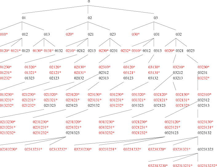
Figure 2: Generating all substrings that begin with 0. Substrings that contain an island are marked with an asterisk and not evaluated further. Multiple consecutive symbols are omitted; only the first instance of the symbol is included.

leaf node		bounded segmentation
leaf	island	copies	$\rho$	1-seg	2-seg	3-seg
010	010	1	2	1	0	0
020	020	2	4	2	1	0
030	030	6	12	6	3	2
0120	0120	2	6	3	1	0
0121	121	see 010
0130	0130	2	6	2	1	1
0131	131	see 020
0210	0210	see 0120
0230	0230	2	6	3	1	1
0232	232	see 010
0310	0310	see 0130
0320	0320	see 0230
01230	01230	1	4	2	1	0
01231	1231	see 0120
01232	232	see 010
01320	01320	1	4	2	1	0
01321	1321	see 0210
02120	02120	1	4	2	1	0
02121	121	see 010
02130	02130	2	8	3	2	1
02131	131	see 020
02310	02310	see 01320
03120	03120	see 02130
03121	121	see 010
03130	03130	2	8	4	2	1
03131	131	see 020
03210	03210	see 01230
03230	03230	1	4	2	1	0
03232	232	see 010
013230	013230	2	10	3	2	1
013231	13231	see 02120
013232	232	see 010
021230	021230	2	10	5	2	1
021231	1231	see 0120
021232	232	see 010
021320	021320	1	5	2	1	0

leaf node		bounded segmentation
leaf	island	copies	$\rho$	1-seg	2-seg	3-seg
021321	1321	see 0210
023120	023120	see 021320
023121	121	see 010
023130	023130	2	10	4	2	1
032131	131	see 020
032132	2132	see 0120
032310	032310	see 013230
0213230	0213230	1	6	3	1	1
0213231	13231	see 02120
0213232	232	see 010
0231230	0231230	1	6	2	1	1
0231231	1231	see 0120
0231232	232	see 010
0231320	0231320	1	6	3	1	1
0231321	1321	see 0210
0313230	0313230	1	6	2	1	1
0313231	13231	see 02120
0313232	232	see 010
0321230	0321230	1	6	3	1	1
0321231	1231	see 0120
0321232	232	see 010
0323120	0323120	see 0213230
0323121	121	see 010
0323130	0323130	see 0313230
0323131	131	see 020
02313230	02313230	2	14	6	3	2
02313231	13231	see 02120
02313232	232	see 010
03231230	03231230	2	14	7	3	2
03231231	1231	see 0120
03231232	232	see 010
03231320	03231320	see 02313230
03231321	1321	see 0210
032313230	03231323	1	8	2	2	1
032313231	13231	see 02120
032313232	232	see 010

Table 1: Segmentations for each leaf in Figure 2. Horizontal rules separate leaves from different levels in the tree.

We now have the following theorem:

Theorem 2.

There exists an algorithm running in $O(m\cdot{}n\cdot{}\log{h})$ time that for any intensity matrix $T$ with maximum value $h$ finds a segmentation ${\mathcal{S}}$ of $T$ of size at most $\frac{11}{6}\cdot(\log_{4}h+1)\cdot OPT+O(1)\cdot(\log_{4}h+1),$ where $OPT$ is the size of a minimal segmentation of $T$.

Proof.

Split $T$ into 0/1/2/3-matrices $P_{\ell}$, for $\ell=0,...,\log_{4}{h}$, such that $T=\sum_{\ell=0}^{\log_{4}{h}}4^{\ell}P_{\ell}$. By Lemma 3, every row of $P_{\ell}$ can be segmented using at most $\rho/2+O(1)$ 1-segments, $\rho/4$ 2-segments, and $\rho/6$ 3-segments. Therefore, the total number of segments required for each $P_{\ell}$ using GreedyRowPacking is at most $\rho/2+\rho/4+\rho/6+O(1)$. The total number of segments required for $T$ is then at most $(\rho/2+\rho/4+\rho/6+O(1))\cdot{}(\log_{4}h+1)$. By Observation 1, $OPT\geq{}\rho/2$. Therefore, the size of the segmentation is at most $(\frac{11}{6}OPT+O(1))\cdot{}(\log_{4}{h}+1)$ which proves the result. ∎

Note that $\frac{11}{6}\log_{4}(h)<\frac{3}{2}\log_{3}(h)<\log_{2}(h)$, so for sufficiently large $OPT$ and $h$, the new algorithm provides the best approximation guarantee and is better by a factor of $\frac{12}{11}$. From a theoretical perspective, Theorem 2 is valuable because it guarantees that solving $P_{\ell}$ matrices (either with the algorithm implicit in Lemma 3 or optimally using the results of [16]) yields an approximation guarantee. From an empirical perspective, preliminary experimental results indicated that using base $b=4$ is no better than using base $b=3$ in practice, and we did not pursue this approach further in our experiments (see Section 4).

2.3 Even higher bases?

In theory, our approach could be taken further, using bases $b=5,6,\dots$. There are two obstacles to doing so. First, how to find a good segmentation of a matrix with entries in $0,\dots,b-1$? One can find the optimal segmentation in time $O(mn^{2b-4})$ [16], but this quickly becomes computationally infeasible. Are there faster algorithms?

Secondly, would using an optimal segmentation give a good approximation? This is not immediately clear, and in fact, the following example shows that the approximation factor is not much better than $2\log_{b}(h)$.

Theorem 3.

Consider any approximation algorithm that obtains a segmentation of $T$ by decomposing $T$ into $1+\log_{b}{h}$ matrices $P_{\ell}$ and then combining segmentations of each $P_{\ell}$. Any such algorithm can yield an approximation factor no better than $\frac{(2b-2)}{b}\cdot\log_{b}{h}+\frac{1}{b}$ in the worst case, even for a single-row problem.

Proof.

Define for $\ell=0,\dots,k-1$ matrix $P_{\ell}$ to be

$$(1~{}~{}2~{}~{}3~{}~{}4~{}~{}\cdots~{}~{}(b-1)~{}~{}0~{}~{}(b-1)~{}~{}\cdots{}~{}~{}3~{}~{}2~{}~{}1),$$

and set matrix $P_{k}$ to be

$$(0~{}~{}0~{}~{}0~{}~{}0~{}~{}\cdots~{}~{}0~{}~{}1~{}~{}0~{}~{}\cdots{}~{}~{}0~{}~{}0~{}~{}0).$$

Finally, set $T=\sum_{\ell=0}^{k}b^{\ell}P_{\ell}$.

Clearly $P_{\ell}$, for $\ell<k$ requires at least $2(b-1)$ segments in any segmentation, and $P_{k}$ requires one segment, so any segmentation of $T$ obtained with this approach has $2(b-1)k+1$ segments. On the other hand, matrix $T$ can be segmented with just $b$ segments: For $i=1,\dots,b-1$, the $i$th segment has value $(011\cdots 1)_{b}$ in base $b$ and extends from column $i$ to column $2b-i$, and the $b$th segment contains a single $1$ in the column $b$ and is otherwise 0. Hence, a solution obtained with this approach will have an approximation factor of at least $\frac{(2b-2)}{b}\cdot\log_{b}{h}+\frac{1}{b}$. ∎

If higher bases are to be used, then one way to prove an approximation factor would be to generalize Lemmas 1 and 3. Here, we offer the following:

Conjecture 1.

For any matrix $P_{\ell}$ with entries in $0,1,\dots,b-1$, there exists a segmentation of row $i$ of $P_{\ell}$ that uses at most $\frac{1}{2v}\rho_{\ell}^{i}+O(1)$ segments of value $v$, for $v=1,\dots,b-1$.

Notice that Lemmas 1 and 3 prove this conjecture for $b=3,4$. If the conjecture were true, this could be used to obtain a segmentation of $T$ of size $(H_{b-1}OPT+O(1))(\log_{b}(h)+1)$, where $H_{b-1}=1+\frac{1}{2}+\dots+\frac{1}{b-1}$ is the harmonic number. Since $H_{b-1}\approx\ln(b-1)$, this means that the approximation factor is $\approx\ln(h)$ after ignoring some lower-order terms.

While we are not able to prove the conjecture, we can at least show that nothing better is possible.

Lemma 4.

There exists a matrix $P$ with entries in $0,1,\dots,b-1$ such that any segmentation of $P$ uses at least $H_{b-1}\cdot{\rho}/{2}$ segments.

Proof.

Let $P$ be the matrix

$$\left(\begin{array}[]{cccccccc}1&0&1&0&\dots&1&0&1\\ 2&0&2&0&\dots&2&0&2\\ 3&0&3&0&\dots&3&0&3\\ \vdots&\vdots&\vdots&\vdots&\dots&\vdots&\vdots&\vdots\\ b-1&0&b-1&0&\dots&b-1&0&b-1\\ \end{array}\right),$$

where the number of non-zeros in each row, which is the same as $\rho/2$, can be chosen arbitrarily. Assume $P$ has been segmented using $n_{v}$ segments of value $v$.

Consider the $i$th row of $P$, and count not only the markers, but also the amount by which the values at each marker change. Thus, let $\mu_{i}$ be the sum of the changes between consecutive values in row $i$; then $\mu_{i}=i\cdot\rho$. (Similarly as for markers, changes at the leftmost and rightmost end of the matrix are included.) Each segment of value $v$ in row $i$ can only account for up to $2v$ change between consecutive values (namely, at its two ends). Also notice that necessarily $v\leq i$ since all values in row $i$ are at most $i$. So we must have

$$\sum_{v=1}^{i}2v\cdot n_{v}\geq\mu_{i}=i\cdot\rho.$$

How small can $n_{1}+\dots+n_{b-1}$ be, subject to this constraint (as well as the obvious $n_{i}\geq 0$ for all $i$)? This is a linear program, and using duality theory (see e.g. [11]), one can easily see that the optimal primal solution is $n_{v}^{*}=\frac{1}{v}\cdot\rho/2$. (The optimal dual solution assigns $\frac{1}{i(i+1)}$ to row $i<b-1$ and $\frac{1}{b-1}$ to the last row.) The optimal primal (and dual) solution has value $H_{b-1}\cdot\rho/2$. While $n_{v}^{*}$ need not be integral in general, this nevertheless shows that any segmentation cannot be smaller than the value of the optimal primal solution. So any segmentation of $P_{\ell},\ell<k$ requires at least $H_{b-1}\cdot\rho/2$ segments. ∎

Note that the above matrix can in fact be segmentated using $\frac{1}{v}\cdot\rho/2$ segments of value $v$ if $\rho/2$ is a multiple of $2\cdot(b-1)!$. What remains to do to show Conjecture 1 is to show that this matrix is the worst case that could happen.

We suspect that this (or a similar) matrix could also be used to devise a target-matrix where no approximation better than $\approx ln(h)$ is possible with the split-by-base-$b$-approach, but have not been able to find one.

3 Approximation by modifying row-segmentations

Our previous approximation algorithm can be summarized as follows: split the intensity matrix by digits, split each resulting matrix into rows, segment each row and then put the segments together. The second approximation algorithm by Luan et al. [18] uses another approach that is in some sense reverse: split the intensity matrix into rows, segment each row, split each resulting segment into multiple segments by digits, and then put the segments together. The quality of this second approximation depends on two factors: the approximation guarantee and the largest value used by a segment in any of the row-segmentations. Without formally stating it in these terms, Luan et al. proved the following result:

Lemma 5.

(Luan et al. [18]) Assume that for any single-row problem we can find an $\alpha$-approximate solution where all segments have value at most $M$. Then we can compute in polynomial time an $\alpha(\log M+1)$-approximate segmentation of $T$.

Luan et al. used this property by showing that any single-row problem has a 2-approximate solution where any segment has value at most $D$, where the row-difference $D$ is the maximum difference between consecutive elements in a row, or the maximum of the first and last entries in the row, whichever is larger. We can slightly improve on this with two observations. First, any segmentation can be converted into a segmentation with values at most $D$, without adding any new segments. Secondly, values $\alpha<2$ can be found in existing results.

Lemma 6.

Let ${\mathcal{S}}$ be any segmentation of a single-row intensity matrix $T$ with row-difference $D$. Then there exists a segmentation ${\mathcal{S}}^{\prime}$ with $|{\mathcal{S}}^{\prime}|\leq|{\mathcal{S}}|$ for which all segments have value at most $D$.

Proof.

Modify ${\mathcal{S}}$ such that no two segments meet, i.e., if some segment ends at index $i$, then no segment starts at $i+1$. This can always be done ithout increasing th number of segments, see e.g. [4]. Any segment $S$ must then have value $v\leq D$, for if $S$ ends at $i$, then $T[i+1]=T[i]-v$ since no segment starts at $i+1$. ∎

Theorem 4 follows immediately from Lemma 5 and Lemma 6, using $M=D$:

Theorem 4.

There exists a polynomial-time algorithm that, for any intensity matrix $T$ with maximum row-difference $D$, finds a segmentation ${\mathcal{S}}$ of $T$ size at most $\alpha\cdot{}(\log D+1)OPT$. Here $\alpha\leq\frac{24}{13}\approx{}1.846$ in the general case by [5].

If the running time for obtaining an $\alpha$-approximation for the single row problem is $t_{\alpha}$, then this algorithm runs in $O(t_{\alpha}\cdot{}m\cdot{}\log{h})$; the $\alpha\leq\frac{24}{13}$ algorithm can be implemented in $O(h\cdot{}n^{2})$ time. For the general case, this approximation result improves upon the $2\cdot(\log D+1)$ approximation result for the full-matrix problem in [18]. In particular, for $\alpha=\frac{24}{13}$, if $D\leq{}(h^{13}/8)^{1/16}$, then to the best of our knowledge, this is the tightest approximation to the segmentation problem with no restriction on the intensity matrix values.

4 Experimental Results

To examine the impact of our algorithms in practice, we implemented our new approximation algorithms as well as those of [18]. In particular, our experiments use the following algorithms:

1. Alg_b=2: The $(\log_{2}{h}+1)$ approximation algorithm of [18].

2. Alg_b=3: The $\frac{3}{2}\cdot(\log_{3}{h}+1)$ approximation algorithm of Section 2.

3. Alg_α=2: The $2(\log{D}+1)$ approximation algorithm of [18].

4. Alg_α=24/13: The $\frac{24}{13}\cdot(\log{D}+1)$ approximation algorithm of Section 3, which utilizes our implementations of algorithms from [5, 6].

5. OPT: The optimal solution obtained via a recent state-of-the-art exact algorithm of [8] which improves the running time over the related work in [2].

All approximation algorithms were implemented in Java while an implementation of OPT was provided as a binary executable by the author of [8].

Scope of Our Experiments: We restrict our investigation to algorithms with approximation guarantees. Aside from their practical performance, approximation algorithms play an important role by providing an efficient method for checking the quality of solutions provided by heuristics. While heuristics may perform well in practice, their lack of a performance guarantee means that low-quality solutions cannot be ruled out. On the other hand, as demonstrated by previous works [2, 8] and by our experimental work here, computing the optimum is computationally intensive and can require a significant amount of time; moreover, such exact approaches are only possible with intensity matrices of limited size and $h$ values. Therefore, at the very least, approximation algorithms allow one to quickly verify that a heuristic is not producing a poor result; moreover, the approximate solution may indeed provide a satisfactory solution. While a comprehensive comparison involving the large body of literature on heuristic approaches would be of interest, such an undertaking is outside the scope of this current work.

4.1 Data Sets

We use the following test data:

• Data Set I: a real-world data set comprised of $70$ clinical intensity matrices obtained from the Department of Radiation Oncology at the University of California at the San Francisco School of Medicine. The levels are specified in terms of percentages in increments of $20$% of some maximum value. We extract the common factor of $20$ to obtain values in $\{1,2,3,4,5\}$.

• Data Set II: a real-world data set containing a prostate case, a brain case and a head-neck case obtained from the Department of Radiation Oncology at the University of Maryland School of Medicine. This data set consists of $22$ clinical intensity matrices with fractional values specified absolutely; the floor of these values are used for our experiments.

• Data Set III: a synthetic data set of $30$ intensity matrices. Each matrix is obtained as follows: compute the sum of the probability density functions of seven bivariate Gaussians generated from two independent standard univariate Gaussian distributions where the amplitude $A$ and the centers of the distributions are sampled uniformly at random. The distributions are discretized by adding as the value in the $m\times n$-grid the integer part of the corresponding function value. The choice of seven Gaussians and the range of the amplitude (we chose 1-25) was made to ensure some peaks and valleys in the intensity matrix, while keeping the matrices reasonably small for the purposes of computing an optimal solution.

The utility of Data Set III is that it allows for testing on intensity matrices where $D$ values are relatively small compared to $h$. Such data allows us to address our third line of investigation by examining the effect of small $D$ values on the performance of our approximation algorithms. Moreover, testing on matrices with small $D$ values is pertinent assuming improvements in treatment technology. Higher precision MLCs can allow for more fine-grained intensity matrices and current technologies exist for supporting MLCs with up to 60 leaf pairs. Finally, we note that the $h$ values used in each of our data sets are fairly small - this is necessary in order for the exact algorithm of [8] to complete within a reasonable amount of time as we discuss in more detail later.

4.2 Results of Experiments

Tables 2-5 below contain the results for each instance of our experimental evaluation. All experiments were conducted on a machine with a $1$ GHz Pentium CPU and $1$ GB of RAM. In Tables 4 & 5, the running times for computing the optimum are also included since these were significant.

Instance	m	n	$h$	$D$	OPT	Algb=2	Algb=3	Algα=2	Algα=24/13
1	20	19	5	5	7	10	8	12	12
2	19	18	5	5	8	11	9	11	11
3	19	14	5	5	9	11	10	15	15
4	19	14	5	5	8	10	10	13	15
5	19	16	5	5	8	12	9	14	13
6	20	16	5	5	8	11	9	12	12
7	20	16	5	5	9	12	9	14	15
8	20	16	5	5	8	12	10	13	13
9	20	11	5	5	7	8	8	12	12
10	27	21	5	5	10	13	14	13	14
11	27	20	5	5	10	12	13	11	11
12	26	18	5	5	8	9	10	12	12
13	26	15	5	5	7	9	9	10	10
14	26	18	5	5	8	11	12	12	14
15	26	17	5	5	8	11	11	10	10
16	26	13	5	5	7	10	9	10	10
17	26	18	5	5	8	11	11	11	11
18	27	20	5	5	8	11	10	10	10
19	21	19	5	5	11	15	12	13	13
20	21	17	5	5	7	9	10	12	12
21	21	15	5	5	8	11	8	11	11
22	20	18	5	5	9	12	9	14	14
23	21	18	5	5	9	11	10	12	12
24	21	15	5	5	6	8	7	9	9
25	21	17	5	5	9	12	9	15	14
26	21	19	5	5	9	13	10	14	12
27	21	21	5	5	11	14	14	13	13
28	21	19	5	5	10	14	13	13	13
29	22	16	5	5	8	11	9	11	11
30	21	11	5	5	5	6	7	7	7
31	20	20	5	5	10	14	13	14	14
32	20	19	5	5	9	11	11	12	13
33	22	15	5	5	8	11	10	10	10
34	21	20	5	5	10	13	12	14	14
35	21	16	5	5	8	9	9	10	10

Table 2: The experimental instances 1-35 of Data Set I with the best result provided by the approximation algorithms underscored.

Instance	m	n	$h$	$D$	OPT	Algb=2	Algb=3	Algα=2	Algα=24/13
36	21	14	5	5	8	11	11	12	12
37	25	18	5	5	7	10	10	11	10
38	25	21	5	5	11	14	13	14	13
39	25	18	5	5	8	11	10	13	12
40	26	19	5	5	11	12	14	20	14
41	26	21	5	5	13	16	15	19	17
42	26	18	5	5	9	11	11	12	12
43	25	18	5	5	8	10	10	11	9
44	25	17	5	5	8	11	10	12	12
45	25	21	5	5	11	15	12	15	15
46	7	7	5	5	5	7	6	7	7
47	7	8	5	5	4	6	4	7	7
48	8	9	5	5	5	8	7	7	7
49	8	8	5	5	5	7	6	7	7
50	8	9	5	5	5	7	6	7	6
51	8	9	5	5	6	9	7	11	11
52	8	9	5	5	5	8	5	6	6
53	8	7	5	5	5	7	5	7	7
54	8	9	5	5	6	8	7	8	8
55	21	17	5	5	8	10	10	10	10
56	20	19	5	5	7	9	8	9	9
57	19	14	5	5	5	7	8	6	6
58	20	18	5	5	7	7	8	9	9
59	20	17	5	5	6	7	7	8	8
60	19	15	5	5	3	5	6	4	4
61	20	18	5	5	8	9	10	10	10
62	21	18	5	5	8	10	10	12	12
63	21	20	5	5	8	10	10	10	10
64	23	19	5	5	11	15	12	16	16
65	23	16	5	5	6	10	8	8	8
66	23	12	5	5	4	6	6	7	7
67	23	18	5	5	8	12	10	13	11
68	23	17	5	5	8	11	9	11	11
69	22	14	5	5	5	7	7	8	7
70	22	16	5	5	7	8	9	9	9

Table 3: The experimental instances 36-70 of Data Set I with the best result provided by the approximation algorithms underscored.

Instance	m	n	$h$	$D$	OPT	Algb=2	Algb=3	Algα=2	Algα=24/13
1	15	16	10	8	8 (0.12)	18	15	12	12
2	15	16	10	8	11 (0.12)	16	15	15	15
3	15	15	10	9	8 (0.07)	15	16	10	10
4	16	13	10	9	7 (0.02)	14	8	10	10
5	16	16	10	9	9 (0.18)	14	14	14	14
6	16	16	10	8	10 (0.08)	21	13	17	15
7	15	13	10	10	5 (0.01)	8	9	10	9
8	23	27	10	9	14 (3.61)	24	21	25	25
9	24	24	10	7	14 (0.32)	21	18	17	19
10	23	32	10	10	16 (1.26)	24	23	23	20
11	23	24	10	8	14 (2.95)	22	20	19	19
12	23	26	10	8	12 (0.24)	25	17	17	18
13	23	33	10	7	16 (2.32)	23	19	19	18
14	23	36	10	10	17 (4.89)	27	24	22	20
15	20	23	10	9	9 (0.12)	14	14	13	14
16	20	19	9	8	10 (0.02)	14	16	12	13
17	20	22	10	10	10 (0.08)	15	13	13	13
18	20	22	10	9	10 (0.98)	15	17	16	15
19	20	21	10	7	10 (0.07)	16	14	15	14
20	20	19	10	6	9 (0.03)	14	12	11	13
21	20	23	10	10	11 (3.24)	17	16	19	19
22	21	20	10	10	10 (0.36)	17	17	18	15

Table 4: The experimental instances using Data Set II with the best result provided by the approximation algorithms underscored. The running time in CPU seconds (rounded to the nearest integer) for OPT is provided in parentheses.

Instance	m	n	$h$	$D$	OPT	Algb=2	Algb=3	Algα=2	Algα=24/13
1	57	64	23	2	26 (21485)	50	44	30	29
2	54	58	25	2	26 (141)	49	46	32	30
3	57	58	24	2	23 (5)	42	38	28	26
4	61	57	22	2	23 (17)	42	42	25	25
5	56	57	24	2	22 (1037)	41	37	25	25
6	59	51	20	2	22 (6)	40	39	23	23
7	50	67	24	2	29 (9260)	56	49	34	34
8	69	62	25	2	24 (692)	47	44	30	30
9	62	64	18	2	19 (2)	36	34	20	21
10	59	59	23	2	28 (120822)	54	49	32	32
11	51	51	23	2	21 (15)	40	37	25	22
12	59	60	23	2	25 (8)	47	46	28	27
13	49	50	23	2	20 (25)	38	35	26	25
14	59	45	23	2	19 (104)	34	33	22	22
15	46	53	18	2	22 (2)	42	40	27	23
16	53	63	21	2	22 (11)	45	40	24	24
17	49	66	24	2	24 (848)	45	41	29	29
18	64	64	25	2	24 (6)	44	43	33	31
19	53	53	25	2	22 (121)	41	40	27	25
20	51	57	25	2	23 (564)	45	42	28	24
21	50	46	24	2	19 (3)	35	33	26	22
22	61	58	24	2	25 (5060)	48	44	26	26
23	57	62	19	2	22 (3)	43	38	26	22
24	58	65	21	2	26 (53)	51	44	27	29
25	59	45	24	2	21 (4)	38	35	26	26
26	54	50	15	2	19 (1)	34	33	20	20
27	67	61	20	2	17 (3)	32	29	19	19
28	63	64	25	2	26 (506)	50	46	31	31
29	54	60	18	2	21 (1)	43	38	24	23
30	63	58	24	2	23 (317)	45	42	26	25

Table 5: The experimental instances using Data Set III with the best result provided by the approximation algorithms underscored. The running time in CPU seconds (rounded to the nearest integer) for OPT is provided in parentheses.

4.3 Analysis & Discussion

Table 6 summarizes the performance of our approximation algorithms by enumerating the number of instances in which each algorithm outperformed all others (excluding OPT) with ties included.

	# Instances	Algb=2	Algb=3	Algα=2	Algα=24/13
Data Set I	70	24  (34.3%)	55  (78.6%)	14  (20.0%)	18  (25.7%)
Data Set II	22	3   (13.6%)	9   (40.9%)	11  (50.0%)	12  (54.5%)
Data Set III	30	0   (0.0%)	0   (0.0%)	16  (53.3%)	28  (93.3%)

Table 6: The number of instances where each of approximation algorithms achieves the smallest segmentation with ties included. The largest value in each row is bolded.

In testing our algorithms, we focus on three questions:

1. How do our improved algorithms compare against their older counterparts in [18]?

2. How do the algorithms with an $O(\log{h})$ approximation guarantee compare to those with an $O(\log{D})$ approximation guarantee?

3. How do these approximation algorithms compare against the optimum solution?

Question 1: With respect to our first question, Table 6 illustrates that Alg_b=3 and Alg_α=24/13 outperform on a larger number of instances than the algorithms of [18] in all three data sets for a total of $95$ out of $122$ instances (77.8%). In particular, Alg_b=3 ties or outperforms all other approximation algorithms in $55$ out of the $70$ instances (78.5%) in Data Set I while Alg_α=24/13 ties or outperforms all other approximation algorithms in $12$ out of the $22$ instances (54.5%) in Data Set II and in $28$ out of the $30$ instances (93.3%) in Data Set III. We also enumerate the number of times one of our new algorithms outperforms an older algorithm on an instance-by-instance basis; this comparison is summarized in Table 7 along with ties (percentages along a row may not sum exactly to 100% due to rounding). The results indicate that our new algorithms perform better than their older counterparts on a significant number of instances.

	Algb=2 outperforms Algb=3	Algb=3 outperforms Algb=2	Ties
Data Set I	12  (17.1%)	40  (57.1%)	18  (25.7%)
Data Set II	4  (18.2%)	15  (68.2%)	3  (13.6)
Data Set III	0  (0.0%)	29  (96.7%)	1  (3.3%)
	Algα=2 outperforms Alg${}_{\alpha=\frac{24}{13}}$	Alg${}_{\alpha=\frac{24}{13}}$ outperforms Algα=2	Ties
Data Set I	5  (7.1%)	12  (17.1%)	53  (75.7%)
Data Set II	5  (22.7%)	8  (36.4%)	9  (40.9%)
Data Set III	2  (6.7%)	14  (46.7%)	14  (46.7%)

Table 7: An instance-by-instance comparison of old vs. new $O(\log{h})$ algorithms, old vs. new $O(\log{D})$ algorithms.

Given these positive results, we also wish to know by how much we improve. We look at the number of segments required by an algorithm per instance and calculate the ratio of these two values; the average (Ave.), median (Med.), minimum (Min.) and maximum (Max.) ratios over all instances is reported in Table 8. These values demonstrate that Alg_b=3 performs substantially better than Alg_b=2 overall judging by both the average and median values. In the case of Alg_α=24/13 and Alg_α=2, our gains are smaller, yet we still observe a small overall improvement judging by the average values.

		Ratio of Algb=3 over Algb=2	Ratio of Alg${}_{\alpha=\frac{24}{13}}$ over Algα=2
Data Set I	Ave.	0.9262	0.9860
	Med.	0.9161	1.0000
	Min.	0.6250	0.7000
	Max.	1.2000	1.1667
Data Set II	Ave.	0.9074	0.9878
	Med.	0.8990	1.0000
	Min.	0.5714	0.8333
	Max.	1.1429	1.1818
Data Set III	Ave.	0.9280	0.9650
	Med.	0.9230	1.0000
	Min.	0.8627	0.8462
	Max.	1.0000	1.0741

Table 8: Average, median, minimum and maximum ratios measuring the extent of our improvements.

Question 2: Next we address our second question regarding the performance of the algorithms with an $O(\log{h})$ approximation guarantee versus those with an $O(\log{D})$ approximation guarantee. We restrict ourselves to a comparison of Alg_b=3 and Alg_α=24/13 given the results of the previous discussion. Table 9 provides the results of our comparison on an instance-by-instance basis. As before, we also calculate the average, median, minimum and maximum ratios on a per-instance basis of Alg_α=24/13 over Alg_b=3; these statistics are in Table 10.

	Algb=3 outperforms Alg${}_{\alpha=\frac{24}{13}}$	Alg${}_{\alpha=\frac{24}{13}}$ outperforms Algb=3	Ties
Data Set I	47 (67.1%)	6 (8.6%)	17 (24.3%)
Data Set II	7 (31.8%)	9 (40.9%)	6 (27.3%)
Data Set III	0 (0.0%)	30 (100.0%)	0 (0.0%)

Table 9: An instance-by-instance comparison of Alg_b=3 and Alg_α=24/13.

	Average	Median	Minimum	Maximum
Data Set I	1.1650	1.1111	0.4444	1.8889
Data Set II	0.9810	1.000	0.6250	1.2500
Data Set III	0.6413	0.6526	0.5714	0.7429

Table 10: Average, median, minimum and maximum ratios of Alg_α=24/13 over Alg_b=3.

We can tentatively draw some conclusions from our analysis. We observe that when $h$ and $D$ are relatively equal, the $\frac{3}{2}\cdot{}(\log_{3}{h}+1)$ approximation can yield superior performance in practice judging by both the instance-by-instance comparison in Table 9 and the average and median values of Table 10; this is certainly the case for Data Set I. However, as Data Set II illustrates, there are exceptions and neither algorithm is clearly superior here. For the case where $D$ is significantly smaller than $h$, all statistics suggest that the $24/13\cdot{}(\log{D}+1)$ approximation can yield substantially better solutions.

Question 3: We address our third question by examining the performance of our approximation algorithms against the optimum number of segments. Table 11 provides the average, the median, the worst, the best, and the best (the smallest) theoretical approximation factor achieved by each algorithm over each data set. We observe that the theoretical values appear pessimistic as our approximation algorithms generally do much better. We also note that the theoretical approximation values for Alg_b=3 are worse than that of Alg_b=2 since $h$ and $OPT$ are not sufficiently large for our theoretical improvements to emerge. Relatively small $h$ values are required in order to compute the optimum; however, we still observe improved performance from Alg_b=3 despite the pessimistic approximation guarantee. Moreover, we observe that the approximation algorithms never exceed an approximation factor of $2.25$ in practice and the other statistics demonstrate that the approximation factor can be significantly lower. Indeed, by executing all four approximation algorithms, we never exceed an approximation factor of $1.80$ (this worst case occurs in Data Set II with Alg_α=24/13) over all instances in all data sets. Such computations can be performed easily since these algorithms incur low computational overhead. By performing such an operation and taking the best performance on an instance-by-instance basis, the statistics presented in Table 12 can be obtained. In conclusion, the statistics in Tables 11 and 12 show that these algorithms can provide very good approximations to the optimum.

		Algb=2	Algb=3	Algα=2	Algα=24/13
Data Set I	Average	1.34	1.23	1.44	1.41
	Median	1.37	1.24	1.4	1.39
	Worst	1.67	2.00	1.83	1.87
	Best	1.00	1.00	1.10	1.10
	Theory	3.32	3.79	6.64	6.13
Data Set II	Average	1.66	1.49	1.47	1.44
	Median	1.56	1.43	1.43	1.44
	Worst	2.25	2.00	2.00	1.80
	Best	1.40	1.14	1.19	1.12
	Theory	4.17	4.65	7.17	6.62
Data Set III	Average	1.90	1.76	1.17	1.13
	Median	1.90	1.76	1.17	1.12
	Worst	2.05	1.84	1.40	1.29
	Best	1.79	1.65	1.04	1.00
	Theory	4.90	5.29	4.00	3.69

Table 11: Statistics on the approximation factors achieved by the approximation algorithms.

	Average	Median	Worst	Best
Data Set I	1.19	1.18	1.50	1.00
Data Set II	1.35	1.36	1.60	1.13
Data Set III	1.12	1.12	1.29	1.00

Table 12: Statistics on the best approximation factor achieved by running all approximation algorithms on each instance of a data set and taking the best result.

Running Time: Finally, we note the running times of the approximation algorithms are negligible. In particular, all approximation algorithms completed each instance within at most $0.01$ CPU seconds on Data Set I, $0.02$ CPU seconds on Data Set II, and $0.240$ CPU seconds on Data Set III. In contrast, the running time for computing an optimal solution can be significant. For Data Set II, the algorithm of [8] runs in a reasonable amount of time. However, recall that the values in this data set are rounded down - this was done to ensure that an optimal solution could be computed. While incorporating another decimal place of the data values improves the accuracy of the treatment solution, the resulting intensity matrices simply cannot be solved optimally in any reasonable amount of time due to an $h$ value that has now become one order of magnitude larger; this is a concern for present-day real-world instances. From a more forward-looking perspective, larger intensity matrices may become feasible as technology advances (MLCs with $60$ leaf pairs currently exist); however, increasing the dimensions of the matrix also increases the running time of the exact algorithm. The impact of these two factors begins to become apparent in Data Set III where computing an optimal solution for certain test cases requires substantial CPU time (hundreds to thousands of CPU seconds - see Table 5) for moderately larger matrices and for $h\leq{}25$. Therefore, while exact algorithms like [8] are an extremely valuable approach to solving these problems, their utility may be limited.

5 Conclusion

We provided new approximation algorithms for the full-matrix segmentation problem. We first showed that the single-row segmentation problem is fixed-parameter tractable in the largest value of the intensity matrix. Using this yields provably good approximate segmentations for the full matrix, after suitably splitting either the intensity matrix or approximate segmentations of its rows according to some base-$b$ representation. Finally, our experimental results demonstrate that our theoretical improvements yield new algorithms that, in both the $O(\log{h})$ and $O(\log{D})$ cases, significantly outperform previous approximation algorithms in practice and can achieve reasonable approximations to the optimal solution, especially if executed in concert.

It may be of interest to explore the case of $b\geq 4$. Can approximation algorithms that perform better in practice be obtained? Are further heuristic improvements possible, such that empirical performance in practically relevant cases is increased, while maintaining desirable theoretical approximation guarantees? Can we more exactly determine the threshhold where the $O(\log{h})$ approximation and $O(\log{D})$ approximation lead to differing performance in practice? Finally, a comprehensive comparison of heuristic and approximation algorithms is an interesting avenue of future work.

Acknowledgements: We thank Baruch Schieber for his helpful correspondence with regard to [5]. We also thank Sebastian Brand and Natashia Boland for graciously providing the implementation work in [8]. Finally, we thank Samuel Fiorini for bringing to our attention the work done in [16].

References

- [1] D. Baatar. Matrix Decomposition with Times and Cardinality Objectives: Theory, Algorithms and Application to Multileaf Collimator Sequencing. PhD Thesis, Universität Kaiserslautern, Kaiserslautern, Germany, August 2005.
- [2] D. Baatar, N. Boland, S. Brand, P. Stuckey. Minimum Cardinality Matrix Decomposition into Consecutive-Ones Matrices: CP and IP Approaches. Proc. of the Int. Conf. Integration of AI and OR Techniques in Constraint Programming for Combinatorial Optimization Problems (CPAIOR), 1-15, 2007.
- [3] D. Baatar and H. W. Hamacher. New LP model for Multileaf Collimators in Radiation Therapy. Contribution to the Conference ORP3, Universit¨t Kaiserslautern, 2003.
- [4] D. Baatar, W. Hamacher, M. Ehrgott and G. J. Woeginger. Decomposition of Integer Matrices and Multileaf Collimator Sequencing. Discrete Applied Mathematics, 152, 6-34, 2005.
- [5] N. Bansal, D. Coppersmith, B. Schieber. Minimizing Setup and Beam-On Times in Radiation Therapy. In Proceedings of APPROX, 2006.
- [6] A. Bar-Noy, R. Bar-Yehuda, A. Freund, J. Naor and B. Schieber. A Unified Approach to Approximating Resource Allocation and Scheduling. In Proc. of STOC, 2000.
- [7] T. Biedl, S. Durocher, H. H. Hoos, S. Luan, J. Saia, and M. Young. Fixed-Parameter Tractability and Improved Approximations for Segment Minimization. Preprint arXiv:0905.4930, 2009.
- [8] S. Brand:. The Sum-of-Increments Constraint in the Consecutive-Ones Matrix Decomposition Problem. Proc. of the Symp. on Applied Computing (SAC), 1417-1418, 2009.
- [9] T. R. Bortfeld, D. L. Kahler, T. J. Waldron, and A. L. Boyer. X-Ray Field Compensation with Multileaf Collimators. International Journal of Radiation Oncology, Biology, Physics, 28(3), 723-730, 1994.
- [10] D.Z. Chen, X.S. Hu, S. Luan, S.A. Naqvi, C. Wang, and C.X. Yu. Generalized Geometric Approaches for Leaf Sequencing Problems in Radiation Therapy. Proc. 15th Intl. Symp. on Algorithms and Computation (ISAAC), 271-281, 2004.
- [11] V. Chvátal. Linear Programming. Freeman and Company, New York. 1983.
- [12] M. J. Collins, D. Kempe, J. Saia, and M. Young. Non-Negative Integral Subset Representations of Integer Sets. Information Processing Letters 101(3), 129-133, 2007.
- [13] C. Cotrutz and L. Xing. Segment-Based Dose Optimization Using a Genetic Algorithm. Physics in Medicine and Biology, 48, 2987-2998, 2003.
- [14] J. Dai and Y. Zhu. Minimizing the Number of Segments in a Delivery Sequence for Intensity-Modulated Radiation Therapy with a Multileaf Collimator. Medical Physics, 28(10), 2113-2120, 2001.
- [15] K. Engel. A New Algorithm for Optimal Multileaf Collimator Field Segmentation. Discrete Applied Mathematics, 152, 35-51, 2005.
- [16] T. Kalinowski. The complexity of minimizing the number of shape matrices subject to minimal beam-on time in multileaf collimator field decomposition with bounded fluence. Discrete Applied Mathematics, 157(9), 2089-2104, 2009.
- [17] W. Pribitkin. Simple Upper Bounds for Partition Functions. The Ramanujan Journal. Online at: http://www.springerlink.com/content/d65348128235x7m1/, 2007.
- [18] S. Luan, J. Saia and M. Young. Approximation Algorithms for Minimizing Segments in Radiation Therapy. Information Processing Letters, 101, 239-244, 2007.
- [19] R.A.C. Siochi. Minimizing Static Intensity Modulation Delivery Time Using an Intensity Solid Paradigm, International Journal of Radiation Oncology, Biology, Physics, 43, 671 680, 1999.
- [20] G. Wakea, N. Boland, L. Jennings. Mixed Integer Programming Approaches to Exact Minimization of Total Treatment Time in Cancer Radiotherapy using Multileaf Collimators. Computers and Operations Research, 36(3), 795-810, 2009.
- [21] P. Xia and L. Verhey. Multileaf Collimator Leaf Sequencing Algorithm for Intensity Modulated Beams with Multiple Static Segments. Medical Physics, 1998.