Renormalization vs Strong Form Factors for One Boson Exchange Potentials.

Abstract

We analyze the One Boson Exchange Potential from the point of view of Renormalization theory. We show that the nucleon-meson Lagrangean while predicting the NN force does not predict the NN scattering matrix nor the deuteron properties unambiguously due to the appearance of short distance singularities. While the problem has traditionally been circumvented by introducing vertex functions via phenomenological strong form factors, we propose to impose physical renormalization conditions on the scattering amplitude at low energies. Working in the large $N_{c}$ approximation with $\pi$,$\sigma$,$\rho$ and $\omega$ mesons we show that, once these conditions are applied, results for low energy phases of proton-neutron scattering as well as deuteron properties become largely insensitive to the form factors and to the vector mesons yielding reasonable agreement with the data and for realistic values of the coupling constants.

I Introduction

The One Boson Exchange (OBE) Potential has been a cornerstone for Nuclear Physics during many years. It represents the natural generalization of the One Pion Exchange (OPE) potential proposed by Yukawa Yukawa (1935), and also the scalar meson potential introduced by Johnson and Teller Johnson and Teller (1955). With the advent of vector mesons these degrees of freedom were included as well Bryan and Scott (1964, 1967, 1969); Partovi and Lomon (1970). Actually, Regge theory yields such a potential within a suitable approximation Nagels et al. (1978). The disturbing short distance divergences were first treated by using a hard core boundary condition Bryan and Scott (1964, 1967, 1969) and it was soon realized that divergences in the potential could be treated by introducing phenomenological form factors mimicking the finite nucleon size Ueda and Green (1968). The field theoretical OBE model of the NN interaction Erkelenz (1974); Machleidt et al. (1987) includes all mesons with masses below the nucleon mass, i.e., $\pi$, $\eta$, $\rho(770)$ and $\omega(782)$. We refer to Ref. Machleidt (1989, 2007) for accounts of the many historical revolves of the problem. An important lesson from these developments has been that the non-perturbative nature of the NN force is better handled in terms of quantum mechanical potentials at low energies where relativistic and nonlocal effects contribute at the few percent level. Although such a framework has remained a useful, appealing and accurate phenomenological model after a suitable introduction of phenomenological strong form factors Machleidt et al. (1987); Machleidt (2001) it is far from being a complete description of the intricacies of the nuclear force. The highly successful Partial Wave Analysis (PWA) of the Nijmegen group Stoks et al. (1993) while providing a spectacular fit with $\chi^{2}/{\rm DOF}<1$ comprising a large body of pn and pp scattering data checks mainly OPE and some contributions from other mesons, since the interaction below $1.4{\rm fm}$ is parameterized by an energy dependent square well potential.

A traditional test to NN forces in general and OBE potentials in particular has been NN scattering in the elastic region. In such a situation relative NN de Broglie wavelengths larger than half a fermi are probed; a factor of two bigger scale than the Compton wavelengths of the vector and heavier mesons. However, while from this simple minded argument we might expect those mesons to play a marginal role, OBE potentials have traditionally been sensitive to short distances requiring a unnatural fine tuning of the vector meson coupling. As a consequence there has been some inconsistency between the couplings required from meson physics, SU(3) or chiral symmetry on the one hand and those from NN scattering fits on the other hand (see also Stoks and Rijken (1997); Furnstahl et al. (1997); Papazoglou et al. (1999)). Part of the disagreement could only be overcome after even shorter scales were explicitly considered Janssen et al. (1994, 1996). A more serious shortcoming stems from the use of strong form factors which have mainly been phenomenologically motivated and loosely related to the field theoretical meson-baryon Lagrangean from which the meson exchange picture is derived. It is therefore not exaggerated to say that strictly speaking the OBE potentials have not been solved yet. Of course, this may appear as a mathematically interesting problem with no relevance to the physics of NN interactions. However, as we will see, the Meson-Nucleon Lagrangean itself while providing the NN OBE potential from the Born approximation, does not predict the NN S-matrix and the deuteron unambiguously beyond perturbation theory from the OBE potential. The unspecified information in the Lagrangean can be advantageously tailored to fit the data in the low energy region. We will also show that once this is done, the vertex functions play a minor role, with a fairly satisfactory description of central waves and the deuteron.

It is notorious that the OBE potentials although exponentially suppressed with the corresponding meson mass, $\sim e^{-mr}$, are by themselves large at short distances and mostly even diverge as $1/r^{3}$. For a singular potential, i.e. a potential fulfilling $\lim_{r\to 0}2\mu|V(r)|r^{2}=\infty$ Case (1950); Frank et al. (1971), the Hamiltonian is unbounded from below preventing the existence of a stable two nucleon bound state when $\lim_{r\to 0}2\mu V(r)r^{2}<-1/4$. Of course, the singularity is unphysical as it corresponds to the interaction of two point-like static classical particles and not to extended nucleons with a finite size of about half a fermi . From a quantum mechanical viewpoint, however, the relative NN de Broglie wavelength provides the limiting resolution scale physically operating in the problem. This suggests that finite nucleon size effects should also play a marginal role in NN scattering in which case it should be possible to formulate the problem without any explicit reference to form factors. In fact, as we will explicitly demonstrate Renormalization is the natural mathematical tool to implement the physically desirable decoupling of short distance components of the interaction at the energies involved in NN elastic scattering.

Within the NN system the problem of infinities has traditionally been cured Ueda and Green (1968) by the introduction of phenomenologically or theoretically motivated strong form factors in each meson-nucleon vertex, $\Gamma_{mNN}(q^{2})$ ($m=\pi,\sigma,\rho,\omega$ etc.) where the off-shellness of the nucleon legs is usually neglected. This procedure somewhat mimics the finite nucleon size but strong form factors are fitted and constrained in practice to NN scattering data and deuteron properties. This corresponds to the replacement of the potential $V_{m}(q)\to V_{m}(q)\left[\Gamma_{mNN}(q)\right]^{2}$ where typically a monopole form is taken for each separate meson $\Gamma_{mNN}(q)=(\Lambda_{mNN}^{2}-m^{2})/(\Lambda_{mNN}-q^{2})$ and generally $\Lambda_{mNN}\sim 1-2{\rm GeV}$ . Due to the long distance distortion introduced by the vertex function deuteron properties impose limitations on the lowest cut-off value $\Lambda_{\pi NN}>1.3{\rm GeV}$ still fitting the result Machleidt et al. (1987).

Because of their fundamental character and the crucial role played in NN calculations there have been countless attempts to evaluate strong form factors by several means, mainly $\Gamma_{\pi NN}(q^{2})$. These include meson theory Woloshyn and Jackson (1972); Gari and Kaulfuss (1984); Kaulfuss and Gari (1983); Flender and Gari (1995); Schutz et al. (1996); Bockmann et al. (1999), Regge models Bryan et al. (1980), chiral soliton models Cohen (1986); Alberto et al. (1990); Christov et al. (1996); Holzwarth and Machleidt (1997), QCD sum rules Meissner (1995) the Goldberger-Treimann discrepancy Coon and Scadron (1990) or lattice QCD Liu et al. (1995); Alexandrou et al. (2007) and quark models Melde et al. (2009). Most calculations yield rather small values $\Lambda_{\pi NN}\sim 800{\rm MeV}$ generating the soft form factor puzzle for the OBE potential for several years since the cut-off could not be lowered below $\Lambda_{\pi NN}=1.3{\rm GeV}$ without destroying the quality of the fits and the description of the deuteron Machleidt et al. (1987). The contradiction was solved by including either $\rho\pi$ exchange Janssen et al. (1993), a strongly coupled excited $\pi^{\prime}(1300)$ state Holinde and Thomas (1990), two pion exchange Haidenbauer et al. (1994) or three pion exchange Ueda (1992). Some of these ways out of the paradox assume the meson exchange picture seriously to extremely short distances. However, as noted in Ref. Holzwarth and Machleidt (1997) the contradiction is misleading since a large cut-off is needed just to avoid a sizable distortion of the OBE potential in the region $r>0.5{\rm fm}$ which can also be achieved by choosing a suitable shape of the form factor. This point was explicitly illustrated by using the Skyrme soliton model form factors Holzwarth and Machleidt (1997). In fact, this conclusion is coherent with the early hard core regularizations Bryan and Scott (1964, 1967, 1969), recent lattice calculations Alexandrou et al. (2007) (where an extremely hard $\Lambda_{\pi NN}\sim 1.7{\rm GeV}$ and a rather flat behaviour are found) and, as we will show, with the renormalization approach we advocate.

The implementation of vertex meson-nucleon functions has also notorious side effects, in particular it affects gauge invariance, chiral symmetry and causality via dispersion relations. As it is widely accepted, besides the description of NN scattering and the deuteron, one of the great successes and confirmations of Meson theory has been the prediction of Meson Exchange Currents (MEC’s) for electroweak processes (see Ericson and Weise (1988); Riska (1989) for reviews and references therein). In the case of gauge invariance, the inclusion of a form-factor introduced by hand, i.e., not computed consistently within meson theory, implies a kind of non-locality in the interaction. This can be made gauge invariant by introducing link operators between two points, thereby generating a path dependence, and thus an ambiguity is introduced. In the limit of weak non-locality the ambiguity is just the standard operator ordering problem, for which no obvious resolution has been found yet. Form factors can also be in open conflict with dispersion relations, particularly if they imply that the interaction does not vanish as a power of the momentum everywhere in the complex plane. We will show that within the renormalization approach, all singularities fall on the real axes and spurious deeply bound states are shifted to the real negative. The extremely interesting issue of analyzing the consequences of renormalization for electroweak processes is postponed for future research.

In the present paper we approach the NN problem for the OBE potential from a renormalization viewpoint. We analyze critically the role played by the customarily used phenomenological form factors. As a viable alternative we carry out the renormalization program to this OBE potential to manifestly implement short distance insensitivity as well as completeness of states by removing the cut-off. In practice, we use the coordinate space renormalization by means of boundary conditions Pavon Valderrama and Ruiz Arriola (2005, 2006a, 2006b). The equivalence to momentum space renormalization using counterterms for regular and singular potentials was discussed in Refs. Pavon Valderrama and Ruiz Arriola (2004); Entem et al. (2008). In order to facilitate and simplify the analysis we will use large $N_{c}$ relations for meson-nucleon couplings Witten (1979); Manohar (1998); Jenkins (1998) which are well satisfied phenomenologically and pick the leading tensorial structures for the OBE potential. In this picture mesons are stable with their mass scaling as $m\sim N_{c}^{0}$, nucleons are heavy with their mass scaling as $M_{N}\sim N_{c}$, the NN potential also scales as $V_{NN}\sim N_{c}$. The OBE component is dominated by the $\pi$, $\sigma$, $\rho$ and $\omega$ mesons Kaplan and Manohar (1997); Banerjee et al. (2002). Further advantages of using this large $N_{c}$ approximation have been stressed in in regard to Wigner and Serber symmetries in Refs. Calle Cordon and Ruiz Arriola (2008a, b); Cordon and Arriola (2009); Arriola and Cordon (2009), in particular the fact that relativistic, spin-orbit and meson widths corrections are suppressed by a relative $1/N_{c}^{2}$ factor suggesting a bold $10\%$ accuracy. However, we hasten to emphasize that despite the use of this appealing and simplifying approximation in the OBE potential we do not claim to undertake a complete large $N_{c}$ calculation since multiple meson exchanges and $\Delta$ intermediate states should also be implemented Banerjee et al. (2002). In spite of this, some of our results fit naturally well within naive expectations of the large $N_{c}$ approach. The coordinate space renormalization scheme is not only convenient and much simpler but it is also particularly suited within the large $N_{c}$ framework, where non-localities in the potential are manifestly suppressed, and an internally consistent multimeson exchange scheme is possible if energy independent potentials are used  Belitsky and Cohen (2002); Cohen (2002).

The paper is organized as follows. In Sect. II we write down a chiral Lagrangean in order to visualize the calculation of the OBE potential in the large $N_{c}$ limit and analyze its singularities. The standard approach to prevent the singularity has been to include form factors to represent vertex functions, an issue which is analyzed critically in Section III where the alternative between fine tuning and the appearance of spurious bound states is highlighted. In Section IV we discuss the physical conditions under which a description of NN scattering makes sense within a renormalization point of view. In addition, we discuss some general features which apply to the solutions of the Schrödinger equation with the local and energy independent large $N_{c}$ OBE potential on the basis of renormalization. In Sect. V we analyze the ${}^{1}S_{0}$ channel from which the scalar meson parameters may be fixed. We also discuss the role played by spurious bound states which appear in this kind of calculations. The deuteron and the corresponding low energy parameters as well as the ${}^{3}S_{1}-^{3}D_{1}$ phase shifts are analyzed in Sect. V. The marginal influence of form factors in the renormalization process is shown in Section  VII. Finally, in Sect. VIII we summarize our main points and conclusions. In appendix A we also review current values for the coupling constants from several sources entering the potential.

II OBE potentials and the need for renormalization

In this section we briefly sketch the well known process of deriving the OBE potential from the nucleon-meson Lagrangean. We appeal a chiral Lagrangean as done in Refs. Stoks and Rijken (1997); Furnstahl et al. (1997); Papazoglou et al. (1999) and keep only the leading $N_{c}$ contributions to the OBE potential due to the tremendous simplification which proves fair enough to illustrate our main point, namely the lack of uniqueness of the S-matrix from the OBE potential. In a more ellaborated version the present calculation should include many other effects such as relativistic corrections, spin-orbit coupling, meson widths, multi-meson exchange and $\Delta$ intermediate states.

II.1 Meson-Nucleon Chiral Lagrangian

We use a relativistic chiral Lagrangean as done in Refs. Stoks and Rijken (1997); Furnstahl et al. (1997); Papazoglou et al. (1999) as a convenient starting point. The $\pi-\sigma$ Lagrangean reads

$${\cal L}_{\sigma\pi}^{\rm kin} = \frac{\sigma^{2}}{4}\langle\partial^{\mu}U^{\dagger}\partial_{\mu}U^{\dagger}\rangle+\frac{1}{2}\partial^{\mu}\sigma\partial_{\mu}\sigma$$ (1)

$$- V(\sigma)-\frac{\sigma m_{\pi}^{2}}{4}\langle U+U^{\dagger}\rangle\,,$$

where $U(x)=e^{i\vec{\tau}\cdot\pi/f_{\pi}}$ is the non-linearly transforming pion field and $\langle,\rangle$ represents the trace in isospin space. The scalar field is invariant under chiral transformations  and the potential is chosen to have a minimum at $\sigma=f_{\pi}$. The sigma mass is then $m_{\sigma}^{2}=V^{\prime\prime}(\sigma)|_{\sigma=f_{\pi}}$, so that the physical scalar field is defined by the fluctuation around the vacuum expectation value, $\sigma=f_{\pi}+s$. $f_{\pi}=92.6~{}{\rm MeV}$ denotes the pion weak-decay constant, ensuring the proper normalization condition of the pseudoscalar fields. The vector mesons kinetic Lagrangeans are represented by Proca fields

$${\cal L}_{\omega}^{\rm kin} = -\frac{1}{4}(\partial^{\mu}\omega^{\nu}-\partial^{\nu}\omega^{\mu})(\partial_{\mu}\omega_{\nu}-\partial_{\nu}\omega_{\mu})+\frac{1}{2}m_{\omega}^{2}\omega^{\mu}\omega_{\mu}\,,$$

$${\cal L}_{\rho}^{\rm kin} = -\frac{1}{4}(\partial^{\mu}\rho^{\nu}-\partial^{\nu}\rho^{\mu})(\partial_{\mu}\rho_{\nu}-\partial_{\nu}\rho_{\mu})+\frac{1}{2}m_{\rho}^{2}\rho^{\mu}\rho_{\mu}\,.$$

and the kinetic nucleon Lagrangian is

$${\cal L}_{N}^{\rm kin}=\bar{N}i\hbox to0.0pt{\hbox to5.30904pt{\hfil/\hfil}\hss}\partial N\,.$$ (3)

The chirally invariant form of the meson-nucleon Lagrangean can be looked up in Ref. Stoks and Rijken (1997). From the vacuum expectation value of the scalar meson we get the nucleon mass $M_{N}=g_{\sigma NN}f_{\pi}$ and the relevant nucleon-meson interaction vertices can be obtained from a chiral Lagrangean Stoks and Rijken (1997); Furnstahl et al. (1997); Papazoglou et al. (1999) and read

$${\cal L}_{\pi NN} = -\frac{g_{\pi NN}}{2\Lambda_{N}}\bar{N}\gamma_{\mu}\gamma_{5}\tau\cdot\partial^{\mu}\pi N\,,$$

$${\cal L}_{\sigma NN} = -g_{\sigma NN}\,\sigma\bar{N}N\,,$$

$${\cal L}_{\rho NN} = -g_{\rho NN}\bar{N}\tau\cdot\rho^{\mu}\gamma_{\mu}N-\frac{f_{\rho NN}}{2\Lambda_{N}}\bar{N}\sigma_{\mu\nu}\tau\cdot\partial^{\mu}\rho^{\nu}N\,,$$

$${\cal L}_{\omega NN} = -g_{\omega NN}\bar{N}\gamma_{\mu}\omega^{\mu}N-\frac{f_{\omega NN}}{2\Lambda_{N}}\bar{N}\sigma_{\mu\nu}\partial^{\mu}\omega^{\nu}N\,,$$

Here and $\Lambda_{N}$ is a mass scale which we take as $\Lambda_{N}=3M_{N}/N_{c}$ with $N_{c}$ the number of colours in QCD. An overview of estimates of couplings from several sources is presented in appendix A. In the large $N_{c}$ limit the Lagrangean simplifies tremendously since one has the following scaling relations Witten (1979) 

$$M_{N} \sim N_{c}\,,$$

$$\Lambda_{N} \sim N_{c}^{0}\,,$$

$$g_{\pi NN} \sim g_{\sigma NN}\sim g_{\omega NN}\sim f_{\rho NN}\sim\sqrt{N_{c}}\,,$$

$$f_{\omega NN} \sim g_{\rho NN}\sim 1/\sqrt{N_{c}}\,,$$

$$m_{\pi} \sim m_{\sigma}\sim m_{\rho}\sim m_{\omega}\sim N_{c}^{0}\,,$$

$$\Gamma_{\sigma} \sim \Gamma_{\rho}\sim 1/N_{c}\,.$$ (5)

The vector/tensor coupling dominance for $\omega$/$\rho$ is well fulfilled phenomenologically (see appendix A). Thus, in the large $N_{c}$ limit it is convenient to pass to the heavy baryon formulation by the transformation

$$N(x)=e^{iM_{N}v\cdot x}B(x)\,.$$ (6)

where $B(x)$ is the heavy iso-doublet baryon field and $v^{\mu}$ a four-vector fulfilling $v^{2}=1$, eliminating the heavy mass term Jenkins and Manohar (1991); Bernard et al. (1992). Choosing $v^{\mu}=(1,0)$ the meson-nucleon Lagrangean becomes

$${\cal L} = -g_{\sigma NN}sB^{\dagger}B+g_{\omega NN}\omega^{0}B^{\dagger}B$$

$$+ g_{\pi NN}B^{\dagger}\sigma_{i}\tau_{a}B\partial^{i}\phi^{a}+\frac{f_{\rho NN}}{2\Lambda_{N}}\epsilon^{ijk}B^{\dagger}\sigma_{i}\tau_{a}B\partial^{j}\rho^{ka}\,.$$

In the large $N_{c}$-limit the contracted $SU(4)$ algebra with the generators given by the total spin $S_{i}=\sum_{A}\sigma_{i}^{A}/2$, the total isospin $T_{a}=\sum_{A}\tau_{a}^{A}/2$ and the Gamow-Teller $X_{ia}=\sum_{A}\sigma_{i}^{A}\tau_{a}^{A}/4$ operators is satisfied Manohar (1998); Jenkins (1998)). One could, of course, have started directly from the heavy-baryon Lagrangean, Eq. (LABEL:eq:heavy-lag), but the connection with chiral symmetry, in particular the relativistic mass relation $M_{N}=g_{\sigma NN}f_{\pi}$ would be lost.

II.2 OBE potentials at leading $N_{c}$

From the heavy-baryon Lagrangean, Eq. (LABEL:eq:heavy-lag), the calculation of the NN potential in momentum space is straightforward Machleidt et al. (1987); Machleidt (2001). However, passing to coordinate space is somewhat tricky since distributional contributions proportional to $\delta(\vec{x})$ and derivatives may appear. We discard them but just assuming that $r>r_{c}$ where $r_{c}$ is a short distance radial cut-off . According to their increasing mass the leading $N_{c}$ contributions to the OBE potentials read

$$V_{\pi}(r) = \frac{1}{12}\vec{\tau}_{1}\cdot\vec{\tau}_{2}\frac{g_{\pi NN}^{2}}{4\pi}\frac{m_{\pi}^{2}}{\Lambda_{N}^{2}}\Big{[}\vec{\sigma}_{1}\cdot\vec{\sigma}_{2}\frac{e^{-m_{\pi}r}}{r}$$ (8)

$$+ S_{12}\frac{e^{-m_{\pi}r}}{r}\left(1+\frac{3}{m_{\pi}r}+\frac{3}{(m_{\pi}r)^{2}}\right)\Big{]}\,,$$

$$V_{\sigma}(r) = -\frac{g_{\sigma NN}^{2}}{4\pi}\frac{e^{-m_{\sigma}r}}{r}\,,$$ (9)

$$V_{\rho}(r) = \frac{1}{12}\vec{\tau}_{1}\cdot\vec{\tau}_{2}\frac{f_{\rho NN}^{2}}{4\pi}\frac{m_{\rho}^{2}}{\Lambda_{N}^{2}}\Big{[}2\vec{\sigma}_{1}\cdot\vec{\sigma}_{2}\frac{e^{-m_{\rho}r}}{r}$$ (10)

$$- S_{12}\frac{e^{-m_{\rho}r}}{r}\left(1+\frac{3}{m_{\rho}r}+\frac{3}{(m_{\rho}r)^{2}}\right)\Big{]}\,,$$

$$V_{\omega}(r) = \frac{g_{\omega NN}^{2}}{4\pi}\frac{e^{-m_{\omega}r}}{r}\,,$$ (11)

where the tensor operator $S_{12}=3\sigma_{1}\cdot\hat{x}\sigma_{2}\cdot\hat{x}-\sigma_{1}\cdot\sigma_{2}$ has been defined. Thus, the structure of the leading large $N_{c}$-OBE potential has the general structure Kaplan and Manohar (1997)

$$V(r)=V_{C}(r)+\tau_{1}\cdot\tau_{2}\left[\sigma_{1}\cdot\sigma_{2}W_{S}(r)+S_{12}W_{T}(r)\right]\,.$$ (12)

Thus, we have as the only non-vanishing components

$$V_{C}(r) = -\frac{g_{\sigma NN}^{2}}{4\pi}\frac{e^{-m_{\sigma}r}}{r}+\frac{g_{\omega NN}^{2}}{4\pi}\frac{e^{-m_{\omega}r}}{r}\,,$$

$$W_{S}(r) = \frac{1}{12}\frac{g_{\pi NN}^{2}}{4\pi}\frac{m_{\pi}^{2}}{\Lambda_{N}^{2}}\frac{e^{-m_{\pi}r}}{r}+\frac{1}{6}\frac{f_{\rho NN}^{2}}{4\pi}\frac{m_{\rho}^{2}}{\Lambda_{N}^{2}}\frac{e^{-m_{\rho}r}}{r}\,,$$

$$W_{T}(r) = \frac{1}{12}\frac{g_{\pi NN}^{2}}{4\pi}\frac{m_{\pi}^{2}}{\Lambda_{N}^{2}}\frac{e^{-m_{\pi}r}}{r}\left[1+\frac{3}{m_{\pi}r}+\frac{3}{(m_{\pi}r)^{2}}\right]$$

$$- \frac{1}{12}\frac{f_{\rho NN}^{2}}{4\pi}\frac{m_{\rho}^{2}}{\Lambda_{N}^{2}}\frac{e^{-m_{\rho}r}}{r}\left[1+\frac{3}{m_{\rho}r}+\frac{3}{(m_{\rho}r)^{2}}\right]\,,$$

At short distances we have

$$V_{C}(r) \to \frac{g_{\omega NN}^{2}-g_{\sigma NN}^{2}}{4\pi}\,\frac{1}{r}\,,$$ (14)

$$W_{S}(r) \to \frac{1}{12}\frac{g_{\pi NN}^{2}m_{\pi}^{2}+2f_{\rho NN}^{2}m_{\rho}^{2}}{4\pi\Lambda_{N}^{2}}\,\frac{1}{r}\,,$$ (15)

$$W_{T}(r) \to \frac{1}{4}\frac{g_{\pi NN}^{2}-f_{\rho NN}^{2}}{4\pi\Lambda_{N}^{2}}\,\frac{1}{r^{3}}\,.$$ (16)

As we see, the potential is singular at short distances except for the very special value $f_{\rho NN}=g_{\pi NN}$ (see Appendix B). While the central $V_{C}$ and spin $W_{S}$ contributions present a mild Coulomb singularity, the tensor force component $W_{T}$ is a more serious type of singularity, a situation appeared already for the simpler OPE potential Pavon Valderrama and Ruiz Arriola (2005).

II.3 The OBE potential and ambiguities in the S-matrix

We will show next that the S-matrix associated to the OBE potential is necessarily ambiguous, precisely because of the short distance $1/r^{3}$ singularity in the non-exceptional situation $g_{\pi NN}\neq f_{\rho NN}$. The exceptional case, $g_{\pi NN}=f_{\rho NN}$ will be treated in Appendix B. We do so by proving that the standard regularity conditions for the wave function do not uniquely determine the solution of the Schrödinger equation. Actually, at short distances, i.e. much smaller than meson masses, $r\ll 1/m$, the NN problem due to the OBE potential corresponds to the interaction of two spin-1/2 magnetic dipoles, namely

$$-\nabla^{2}\Psi_{k}(\vec{x})+U_{dd}(\vec{x})\Psi_{k}(\vec{x})=p^{2}\Psi_{k}(\vec{x})\,,\qquad r\ll 1/m\,,$$

(17)

where the reduced dipole-dipole potential is given by

$$U_{dd}(\vec{x}) = MV_{dd}(\vec{x})=$$ (18)

$$= \pm\frac{R}{r^{3}}\,\left(3\sigma_{1}\cdot\hat{x}\sigma_{2}\cdot\hat{x}-\sigma_{1}\cdot\sigma_{2}\right)\,,$$

with $R$ is a length scale and in our particular case

$$\pm R=\frac{M}{16\pi\Lambda_{N}^{2}}(g_{\pi NN}^{2}-f_{\rho NN}^{2})\,,$$ (19)

the positive or negative sign depends on whether $g_{\pi NN}>f_{\rho NN}$ or $g_{\pi NN}<f_{\rho NN}$ respectively.

Figure 1: The potentials $V_{C}(r)$, $W_{S}(r)$ and $W_{T}(r)$ in ${\rm MeV}$ as a function of the distance (in fm). We include the effect of both exponential, Eq. (31), and monopole Eq. (30) form factors for $\Lambda_{\pi NN}=1300{\rm MeV}$ and $\Lambda_{\pi NN}=2000{\rm MeV}$. All other cut-offs are kept to $\Lambda_{\sigma NN}=\Lambda_{\rho NN}=\Lambda_{\omega NN}=2000{\rm MeV}$.

The above potentials become diagonal in the standard total spin $\vec{S}^{2}$, parity $U_{P}$, isospin $\vec{T}$ and total angular momentum $\vec{J}=\vec{L}+\vec{S}$ basis, so the states are labeled by the spectroscopic notation ${}^{2S+1}L_{J}$. We remind that Fermi-Dirac statistics implies $(-1)^{L+S+T}=-1$. Thus, $\tau_{1}\cdot\tau_{2}=2T(T+1)-3$ and $\sigma_{1}\cdot\sigma_{2}=2S(S+1)-3$. For spin singlet states $S=0$ and $J=L$, the parity is natural $U_{P}=(-1)^{J}$ and one has $S_{12}=0$. For uncoupled spin triplet states $S=1$ one has $J=L$, natural parity $U_{P}=(-1)^{L}$ and $S_{12}=2$. For coupled spin triplet states $S=1$ one has $L=J\pm 1$, unnatural parity $U_{P}=(-1)^{J+1}$ and

$$S_{12}=\begin{pmatrix}-\frac{2(J-1)}{2J+1}&\frac{6\sqrt{J(J+1)}}{2J+1}\\ \frac{6\sqrt{J(J+1)}}{2J+1}&-\frac{2(J+2)}{2J+1}\end{pmatrix}\,.$$ (20)

For the uncoupled spin-triplet channel we have

$$-v_{J}^{\prime\prime}(r)+\left[\frac{2R}{r^{3}}+\frac{J(J+1)}{r^{2}}\right]v_{J}(r) = p^{2}v_{J}(r)\,.$$ (21)

At very short distances we may neglect the centrifugal barrier and the energy yielding

$$-v_{J}^{\prime\prime}(r)\pm\frac{2R}{r^{3}}v_{J}(r)=0\,,\qquad r\ll 1/m,R,1/p\,.$$ (22)

The general solution can be written in terms of Bessel functions. Using their asymptotic expansions we may write at short distances 

$$v_{+,J}(r) \to \left(\frac{r}{R}\right)^{3/4}\left[C_{1R}e^{+4\sqrt{2}\sqrt{\frac{R}{r}}}+C_{2R}e^{-4\sqrt{2}\sqrt{\frac{R}{r}}}\right]\,,$$

$$v_{-,J}(r) \to \left(\frac{r}{R}\right)^{3/4}\left[C_{1A}e^{-4i\sqrt{\frac{R}{r}}}+C_{2A}e^{4i\sqrt{\frac{R}{r}}}\right]\,.$$

Clearly in the repulsive case the regularity condition fixes the coefficient of the diverging exponential to zero, $C_{1R}=0$, whereas in the attractive case both linearly independent solutions are regular and the solution is not unique. In the case of the triplet coupled channel, we have for $r\ll 1/m,R,1/p$, i.e. neglecting centrifugal barrier and energy, the system of two coupled differential equations becomes

$$\begin{pmatrix}-u_{J}^{\prime\prime}(r)\\ -w_{J}^{\prime\prime}(r)\end{pmatrix}\pm\frac{R}{r^{3}}\begin{pmatrix}-\frac{2(J-1)}{2J+1}&\frac{6\sqrt{J(J+1)}}{2J+1}\\ \frac{6\sqrt{J(J+1)}}{2J+1}&-\frac{2(J+2)}{2J+1}\end{pmatrix}\begin{pmatrix}u_{J}(r)\\ w_{J}(r)\end{pmatrix}=0\,.$$

(25)

This system can be diagonalized by going to the rotated basis

$$\begin{pmatrix}v_{1,J}(r)\\ v_{2,J}(r)\end{pmatrix} = \begin{pmatrix}\sqrt{\frac{J}{2J+1}}&-\sqrt{\frac{J+1}{2J+1}}\\ \sqrt{\frac{J+1}{2J+1}}&\sqrt{\frac{J}{2J+1}}\end{pmatrix}\,\begin{pmatrix}u_{J}(r)\\ w_{J}(r)\end{pmatrix},$$ (26)

where the new functions satisfy

$$-v_{1,J}^{\prime\prime}(r)\mp\frac{4R}{r^{3}}v_{1,J}(r) = 0\,,$$ (27)

$$-v_{2,J}^{\prime\prime}(r)\pm\frac{8R}{r^{3}}v_{2,J}(r) = 0\,.$$ (28)

Note that here the signs are alternate, i.e. when one of the short-distance eigenpotentials is attractive the other one is repulsive and viceversa, and hence the type of solutions in Eq. (LABEL:eq:short_bc_r3) can be applied. This means that in general there will be solutions which are not necessarily fixed by the regularity condition at the origin, and thus the OBE potential does not predict the $S-$matrix uniquely. Instead, a complete parametric family of $S-$matrices will be generated depending on the particular choice of linearly independent solutions, which are not dictated by the OBE potential itself.

Thus, some additional information should be given. The traditional way is to introduce form factors to kill the singularity so that the regularity condition fixes the solution uniquely as we discuss in Section III. Another way, which we discuss in the rest of the paper, is to fix directly the integration constants from data with or without form factors. As we will show this way of proceeding does not make much difference showing a marginal influence of form factors (see Sect. VII).

III The standard approach to OBE potentials with form factors

III.1 Features of Vertex Functions

A way out to avoid the singularities is to implement vertex functions in the OBE potentials corresponding to the replacement ($q^{2}=q_{0}^{2}-\vec{q}^{2}$ is the 4-momentum)

$$V_{mNN}(q)\to V_{mNN}(q)\left[\Gamma_{mNN}(q^{2})\right]^{2}\,.$$ (29)

Note that this assumes 1) Off-shell independence and 2) The form factor is accurately known. Standard choices are to take form factors of the monopole Machleidt et al. (1987) and exponential Nagels et al. (1978) parameterizations

$$\Gamma_{mNN}^{\rm mon}(q^{2}) = \frac{\Lambda^{2}-m^{2}}{\Lambda^{2}-q^{2}}\,,$$ (30)

$$\Gamma_{mNN}^{\rm exp}(q^{2}) = \exp\left[\frac{q^{2}-m^{2}}{\Lambda^{2}}\right]\,,$$ (31)

fulfilling the normalization condition $\Gamma_{mNN}(m^{2})=1$. These forms are so constructed as to have the same slope at small values of $q^{2}$ in the large cut-off expansion

$$\Gamma_{mNN}(q^{2})=1+\frac{q^{2}-m^{2}}{\Lambda^{2}}+{\cal O}(\Lambda^{-4})\,.$$ (32)

so that the meaning for the cut-off is similar. In coordinate space this can be easily implemented for Yukawa potentials using

$$Y_{\Lambda}(r)=\int\frac{d^{3}q}{(2\pi)^{3}}\frac{e^{iq\cdot x}}{q^{2}+m^{2}}\left[\Gamma_{mNN}(q^{2})\right]^{2}\,,$$ (33)

yielding

$$Y_{\Lambda}^{\rm mon}(r)=\frac{e^{-mr}}{4\pi r}-\frac{e^{-\Lambda r}}{4\pi r}\left[1+r\frac{\Lambda^{2}-m^{2}}{2\Lambda}\right]\,,$$ (34)

which at short distances becomes finite,

$$Y_{\Lambda}^{\rm mon}(r)=\frac{1}{4\pi}\,\frac{(\Lambda-m)^{2}}{2\Lambda}+{\cal O}(r^{2})\,,$$ (35)

which diverges linearly for $\Lambda\to\infty$. The exponentially regularized Yukawa potential reads

$$Y_{\Lambda}^{\rm exp}(r)=\frac{e^{-mr}}{8\pi r} + \frac{e^{-mr}}{8\pi r}{\rm Erf}\left(\frac{\Lambda^{2}r-4m}{2\sqrt{2}\Lambda}\right)$$ (36)

$$- \frac{e^{mr}}{8\pi r}{\rm Erfc}\left(\frac{\Lambda^{2}r+4m}{2\sqrt{2}\Lambda}\right)\,,$$

where ${\rm Erf}$ and ${\rm Erfc}$ are the error function and complementary error function respectively . For $\Lambda r\ll 1$ we have the finite result

$$Y_{\Lambda}^{\rm exp}(r)=\frac{e^{-2m^{2}/\Lambda^{2}}\Lambda}{\sqrt{2\pi}4\pi}-\frac{m}{4\pi}{\rm Erfc}\left(\frac{\sqrt{2}m}{\Lambda}\right)+{\cal O}(r^{2})\,,$$ (37)

which diverges linearly for $\Lambda\to\infty$. In the limit $\Lambda r\gg 1$ behaves as

$$Y_{\Lambda}^{\rm exp}(r)=\frac{e^{-mr}}{4\pi r}-\frac{e^{-\frac{1}{8}\Lambda^{2}r^{2}}e^{-2m^{2}/\Lambda^{2}}}{\sqrt{2\pi}\Lambda\pi r^{2}}+\dots$$ (38)

and the distortion of the original Yukawa potential is much more suppressed in the exponential than in the case of monopole form factor.

In any case we note the amazing feature that the form factors have a radically different effect on different components of the potential. While $V_{C}$ and $W_{S}$ with a mild $\sim 1/r$ short distance behaviour become finite, the tensor force behaving as $W_{T}\sim 1/r^{3}$ vanishes at the origin after due to the form factors, $W_{T}^{\rm mon}(0)=W_{T}^{\rm exp}(0)=0$. This can be seen from the expression

$$\lim_{r\to 0}\int\frac{d^{3}q}{(2\pi)^{3}}e^{iq\cdot x}\,\frac{\sigma_{1}\cdot q\sigma_{2}\cdot q}{q^{2}+m^{2}}\left[\Gamma_{mNN}(q^{2})\right]^{2}$$

$$=\frac{1}{3}\sigma_{1}\cdot\sigma_{2}\left[\int\frac{d^{3}q}{(2\pi)^{3}}\left[\Gamma_{mNN}(q^{2})\right]^{2}-m^{2}Y_{\Lambda}(0)\right]\,,$$

(39)

which corresponds to take an angular average at short distances. This feature suggests that the impact of the tensor force at short distances should be small and looks clearly against the result of the short distance analysis outlined in Section II where there is a strong mixing at short distances. As we will show in Sect. VI, within the renormalization approach there is no contradiction; physical observables will naturally display a small mixing .

We show in Fig. 1 the potentials $V_{C}(r)$, $W_{S}(r)$ and $W_{T}(r)$ in ${\rm MeV}$ as a function of the distance (in fm). We also include the effect of both exponential, Eq. (31), and monopole Eq. (30) form factors for $\Lambda_{\pi NN}=1.3{\rm GeV}$ and $\Lambda_{\pi NN}=2{\rm GeV}$. All other cut-offs are kept to the values $\Lambda_{\sigma NN}=\Lambda_{\rho NN}=\Lambda_{\omega NN}=2{\rm GeV}$. As we see, the distortion of the tensor component due to the strong form factor takes place already at $r\sim 1{\rm fm}$ for softest cut-off $\Lambda_{\pi NN}=1.3{\rm GeV}$. The key issue here is to decide whether this distortion represents a true physical effect, rather than a mere artifact of the regularization. This boils down to determine if one can visualize finite nucleon size effects when the probing wavelength is not shorter than $0.5{\rm fm}\leq r\leq 1{\rm fm}$. The fact that the monopole and exponential parameterizations agree down to $r\sim 0.5{\rm fm}$ but differ from the bare unregularized potential suggests that one could look for a true physical effect based on model independent distortions in the region slightly above $0.5{\rm fm}$. This point will be analyzed further in Section VII.

Finally, note that the multiplicative manner in which form factors are introduced, although it looks quite natural, does build in correlations which may not reflect the real freedom one has in general; a dynamical calculation need not comply to this factorization scheme.

Figure 2: The ${}^{1}S_{0}$ potential $V_{{}^{1}S_{0}}(r)$ in ${\rm MeV}$ as a function of the distance (in fm) for the different scenarios with large and small $\omega-$couplings. We include the effect of both exponential, Eq. (31), and monopole Eq. (30) form factors for $\Lambda_{\pi NN}=1300{\rm MeV}$. All other cut-offs are kept to $\Lambda_{\sigma NN}=\Lambda_{\rho NN}=\Lambda_{\omega NN}=2000{\rm MeV}$.

III.2 The problem of short distance sensitivity vs spurious bound states

The advantage of using vertex functions is that they make the OBE non-singular at short distances. As a consequence, the choice of the regular solution determines the solution uniquely. In this section we analyze critically the use of form factors which are customarily employed in NN calculations based on the OBE potential. We will see that for natural choices of meson-nucleon parameters (see Appendix A), the NN potential displays short distance insensitivity and at the same time spurious deeply bound states. However, if we insist on not having spurious bound states the resulting description is highly short distance sensitive.

As we have mentioned, NN scattering in the elastic region below pion production threshold involves CM momenta $p<p_{max}=400$ MeV. Given the fact that $1/m_{\omega}\sim 1/m_{\rho}\sim 0.25\mathrm{fm}\ll 1/p_{max}=0.5\mathrm{fm}$ we expect heavier mesons to be irrelevant, and $\omega$ and $\rho$ to be marginally important, even in s-waves, which are most sensitive to short distances. This desirable property has not been fulfilled in the traditional approach to OBE forces. In order to illustrate this, we consider the ${}^{1}S_{0}$ channel, where the potential (without form factor) is

$$V_{{}^{1}S_{0}}(r) = V_{C}(r)-3W_{S}(r)$$ (40)

$$= -\frac{g_{\pi NN}^{2}m_{\pi}^{2}}{16\pi M_{N}^{2}}\frac{e^{-m_{\pi}r}}{r}-\frac{g_{\sigma NN}^{2}}{4\pi}\frac{e^{-m_{\sigma}r}}{r}$$

$$+ \frac{g_{\omega NN}^{2}}{4\pi}\frac{e^{-m_{\omega}r}}{r}-\frac{f_{\rho NN}^{2}m_{\rho}^{2}}{8\pi M_{N}^{2}}\frac{e^{-m_{\rho}r}}{r}\,.$$

We take $m_{\pi}=138$MeV, $M_{N}=939$MeV, $m_{\rho}=770$MeV, $m_{\omega}=783$MeV and $g_{\pi NN}=13.1$, which seem firmly established, and treat $m_{\sigma}$, $g_{\sigma NN}$ and $g_{\omega NN}$ and $f_{\rho NN}$ as fitting parameters. To see the role of vector mesons we note the redundant combination of coupling constants $g_{\omega NN}^{2}-f_{\rho NN}^{2}m_{\rho}^{2}/(2M_{N}^{2})$ which appears in the ${}^{1}S_{0}$ potential when we take $m_{\rho}=m_{\omega}$, a tolerable approximation within the present context. To avoid unnecessary strong correlations we define the effective coupling

$$g_{\omega NN}^{*}=\sqrt{g_{\omega NN}^{2}-\frac{f_{\rho NN}^{2}m_{\rho}^{2}}{2M_{N}^{2}}}\,.$$ (41)

Natural values for the coupling constants $g_{\omega NN}=9-10.5$ and $f_{\rho NN}=14-18$ imply $g_{\omega NN}^{*}=0-7$. In Fig. 2 the potential without and with monopole and exponential vertex functions is depicted for several values of $g_{\omega NN}^{*}$. As we see, the differences start below $1{\rm fm}$ where the standard short distance repulsive core is achieved by large and unnatural values of $g_{\omega NN}^{*}$, and not so much depending on the form factors. On the other hand, if we use the regularized ${}^{1}S_{0}$ potential at $r=0$ and take the natural values for the coupling constants $g_{\omega NN}=9-10.5$ and $f_{\rho NN}=14-18$ the potential at the origin becomes

$$V_{{}^{1}S_{0}}(0)=-(1000-3000){\rm MeV}\,.$$ (42)

which is huge and attractive. The number of states is approximately given by the WKB estimate

$$N_{B}\sim\frac{1}{\pi}\int_{0}^{\infty}\sqrt{-MV_{{}^{1}S_{0}}(r)}dr\,.$$ (43)

which yields numbers around unity. In fact the potential accommodates a deeply bound state, at about

$$E_{B}=-(500-2000){\rm MeV}$$ (44)

This state does not exist in nature and should clearly be ruled out from the description on a fundamental level. On the other hand, we do not expect such state to influence the low energy properties below the inelastic pion production threshold $E_{\rm CM}=175{\rm MeV}$ in any significant manner.

Figure 3: Zero energy wave function for the singlet pn ${}^{1}S_{0}$ channel as a function of distance (in fm) and for the different scenarios with large and small $\omega-$couplings. We include the effect of both exponential, Eq. (31), and monopole Eq. (30) form factors for $\Lambda_{\pi NN}=1300{\rm MeV}$. All other cut-offs are kept to $\Lambda_{\sigma NN}=\Lambda_{\rho NN}=\Lambda_{\omega NN}=2000{\rm MeV}$ This wave function goes asymptotically to $u_{0}(r)\to 1-r/\alpha_{0}$ with $\alpha_{0}=-23.74{\rm fm}$ the scattering length in this channel. The zero at about $r=0.5{\rm fm}$ signals the existence of a spurious bound state.

Table 1: Fits to the ${}^{1}S_{0}$ phase shift of the Nijmegen group Stoks et al. (1994) using the OBE potential without or with strong exponential and monopole form factor. We take $m=138.03{\rm MeV}$, and $g_{\pi NN}=13.1083$ de Swart et al. (1997) and $m_{\rho}=m_{\omega}=770{\rm MeV}$ and fit $m_{\sigma}$, $g_{\sigma NN}$ and $g_{\omega NN}^{*}$. We use $\Lambda_{\pi NN}=1300{\rm MeV}$ and $\Lambda_{\sigma NN}=\Lambda_{\rho NN}=\Lambda_{\omega NN}=2000{\rm MeV}$. $E_{B}$ represents the energy of the (spurious) bound state when it does exist.

	$r_{c}({\rm fm})$	$m_{\sigma}({\rm MeV})$	$g_{\sigma NN}$	$g_{\omega NN}^{*}$	$\chi^{2}/DOF$	$\alpha_{0}({\rm fm})$	$r_{0}({\rm fm})$	$E_{B}({\rm MeV})$
$\Gamma(q^{2})=1$	0	547.55(4)	13.559(8)	19.68(2)	0.869	-23.742	2.702	$-$
$\Gamma(q^{2})=1$	0.1	500.9 (5)	9.61(1)	8.09(2)	0.484	-23.742	2.504	-638
$\Gamma(q^{2})=\Gamma^{\rm exp}(q^{2})$	0	552.57(5)	13.78(2)	19.21(4)	0.664	-23.741	2.703	$-$
$\Gamma(q^{2})=\Gamma^{\rm exp}(q^{2})$	0	525.1(1)	10.41(1)	2.9(1)	0.213	-23.740	2.698	-578
$\Gamma(q^{2})=\Gamma^{\rm mon}(q^{2})$	0	551.7(1)	13.99(1)	19.978 (11)	0.971	-23.741	2.707	$-$
$\Gamma(q^{2})=\Gamma^{\rm mon}(q^{2})$	0	532.5(2)	10.81(1)	3.04(3)	0.241	-23.739	2.696	-597

In the standard approach the scattering phase-shift $\delta_{0}(p)$ is computed by solving the (s-wave) Schrödinger equation in r-space

$$-u^{\prime\prime}_{p}(r)+M_{N}\,V(r)\,u_{p}(r) = p^{2}\,u_{p}(r)$$ (45)

$$u_{p}(r) \to \frac{\sin{\left(pr+\delta_{0}(p)\right)}}{\sin{\delta_{0}(p)}}$$ (46)

with a regular boundary condition at the origin

$$u_{p}(0)=0$$ (47)

This boundary condition obviously implies a knowledge of the potential in the whole interaction region, and it is equivalent to solve the Lippmann-Schwinger equation in p-space. In the usual approach Machleidt et al. (1987); Machleidt (2001) everything is obtained from the potential assumed to be valid for $0\leq r<\infty$. In practice, and as mentioned above, strong form factors are included mimicking the finite nucleon size and reducing the short distance repulsion of the potential, but the regular boundary condition is always kept. One should note, however, that due to the unnaturally large NN ${}^{1}S_{0}$ scattering length ($\alpha_{0}\sim-23{\rm fm}$), any change in the potential $V\to V+\Delta V$ has a dramatic effect on $\alpha_{0}$, since one obtains

$$\Delta\alpha_{0}=\alpha_{0}^{2}M_{N}\int_{0}^{\infty}\Delta V(r)u_{0}(r)^{2}\mathrm{d}r$$ (48)

a quadratic effect in the large $\alpha_{0}$. This implies that potential parameters must be fine tuned, and in particular the short distance physics. To illustrate this we make a fit the np data of Ref. Stoks et al. (1994). The results using the OBE potential without or with strong exponential and monopole form factor  are presented in Table 1. In all cases we have at least two possible but mutually incompatible scenarios. An extreme situation corresponds to the case with no form factors . The small errors should be noted, in harmony with the fine tuning displayed by Eq. (48) and the corresponding couplings and scalar mass are determined to high accuracy but turn out to be incompatible. This is just opposite to our expectations and we may regard these fits, despite their success in describing the data, as unnatural. The ambiguity in these solutions are typical of the inverse scattering problem, and has to do with the number of bound states allowed by the potential. Actually, this can be seen from Fig. 3 where the zero energy wave function is represented. According to the oscillation theorem, the number of interior nodes determines the number of bound states. Thus, the larger values of $g_{\omega NN}^{*}$ correspond to a situation with no-bound states since $u_{0}(r)$ does not vanish, whereas for the smaller $g_{\omega NN}^{*}$ values one has a bound state as $u_{0}(r)$ has a zero, which energy can be looked up in Table 1. Of course, such a bound state does not exist in nature and it is thus spurious. On the other hand they always take place at more than twice the maximum energy probed in NN scattering, $E_{\rm CM}=175{\rm MeV}$, and we should not expect any big effect from such an state. Note that despite the net repulsive $\omega$-vector and attractive $\rho$-tensor couplings, the total potential would not be repulsive at short distances with or without form factors in the solution with natural couplings and a spurious bound state; the net short distance repulsion comes about only in the solution with unnaturally large coupling (see Fig. 2).

From the table 1 one can clearly understand the usually too large values of the $g_{\omega NN}$ coupling constant as compared to those from SU(3) symmetry $g_{\omega NN}\sim 9$ or from the radiative decay $\omega\to e^{+}e^{-}$ yielding $g_{\omega NN}=10.2(4)$. Using the definition of $g_{\omega NN}^{*}$, Eq. (41), we get for $f_{\rho NN}=14-18$ large values of $g_{\omega NN}=20-22$ for the case with no bound state, whereas more natural values $g_{\omega NN}=8.5-10.5$ are obtained for the case with one (spurious) bound state.

IV Boundary condition renormalization and ultraviolet completeness

According to the discussion of Sect. II.3 the short distance $1/r^{3}$ singularity of the OBE potential makes the solution ambiguous, and thus there is a flagrant need of additional information not encoded in the potential itself. Of course, once we realize the freedom of choosing suitable linear combinations of independent solutions, we may question how general this choice can be, even if the potential is not singular. In this Section we derive constraints on the short distance boundary condition. As mentioned already, we work with energy independent potentials. In this section we show what this requirement implies for the renormalization program. Using the potential of Eq. (12) we solve the Schrödinger equation,

$$-\frac{1}{M}\nabla^{2}\Psi_{k}(\vec{x})+V(\vec{x})\Psi_{k}(\vec{x})=E_{k}\Psi_{k}(\vec{x})\,,$$ (49)

where $\Psi(\vec{x})$ is a spin-isospin vector with 4x4=16 components, which usually satisfies the out-going wave boundary condition,

$$\Psi_{k}(\vec{x})\to\left[e^{i\vec{k}\cdot\vec{x}}+f(\hat{k}^{\prime},\hat{k})\frac{e^{ikr}}{r}\right]\chi_{t,m_{t}}^{s,m_{s}}\,,$$ (50)

with $f(\hat{k}^{\prime},\hat{k})$ the quantum mechanical scattering matrix amplitude and $\chi_{t,m_{t}}^{s,m_{s}}$ a 4x4 total spin-isospin state. We apply a radial cut-off $r_{c}$ and consider that the local potential $V(\vec{x})$ is valid for the long distance region $r>r_{c}$. The precise form of the interaction for the short distance region $r<r_{c}$ is not necessary as the limit $r_{c}\to 0$ will be taken at the end. To fix ideas we assume an energy independent non-local potential, as we expect genuine energy dependence to show up as sub-threshold inelastic (e.g. pion production) effects. Any distributional terms $\sim\delta(\vec{x})$ arising from the long distance potential $V(\vec{x})$ are necessarily included in the inner region, $r<r_{c}$. The inner wave function $\Phi_{k}(\vec{x})$ satisfies

$$-\frac{1}{M}\nabla^{2}\Phi_{k}(\vec{x})+\int d^{3}x^{\prime}V(\vec{x}^{\prime},\vec{x})\Phi_{k}(\vec{x}^{\prime})=E_{k}\Phi_{k}(\vec{x})\,,$$ (51)

and will be assumed to vanish at the origin. Using standard manipulations and the Green identity we get for the inner and outer regions

$$(E_{p}-E_{k})\int_{r<r_{c}}d^{3}x\Phi_{k}^{\dagger}(\vec{x})\Phi_{p}(\vec{x})$$ (52)

$$= \int d\vec{S}\left[\vec{\nabla}\Phi_{k}^{\dagger}(\vec{x})\Phi_{p}(\vec{x})-\Phi_{k}^{\dagger}(\vec{x})\vec{\nabla}\Phi_{p}(\vec{x})\right]\Big{|}_{r=r_{c}}\,,$$

and

$$(E_{p}-E_{k})\int_{r>r_{c}}d^{3}x\Psi_{k}^{\dagger}(\vec{x})\Psi_{p}(\vec{x})$$ (53)

$$= -\int d\vec{S}\left[\vec{\nabla}\Psi_{k}^{\dagger}(\vec{x})\Psi_{p}(\vec{x})-\Psi_{k}^{\dagger}(\vec{x})\vec{\nabla}\Psi_{p}(\vec{x})\right]\Big{|}_{r=r_{c}}\,,$$

respectively where the difference in sign form the inner to the outer integration comes from opposite orientations in the integration surface. Clearly, orthogonality of states in the whole space for different energies,

$$\int_{r<r_{c}}d^{3}x\Phi_{k}^{\dagger}(\vec{x})\Phi_{p}(\vec{x})+\int_{r>r_{c}}d^{3}x\Psi_{k}^{\dagger}(\vec{x})\Psi_{p}(\vec{x})=0\,,$$ (54)

can be achieved by setting the general and common boundary condition,

$$\partial_{r}\Phi_{p}(\hat{x}r_{c}) = L_{p}(\hat{x}r_{c})\Phi_{p}(\hat{x}r_{c})$$

$$\partial_{r}\Psi_{p}(\hat{x}r_{c}) = L_{p}(\hat{x}r_{c})\Psi_{p}(\hat{x}r_{c})\,.$$ (55)

Here, $L_{p}(\hat{x}r_{c})$ is a self-adjoint matrix which may depend on energy, and may be chosen to commute with the symmetries of the potential $V(\vec{x})$ . Deriving with respect to the energy the inner boundary condition, Eq. (52), i.e. taking $E_{p}=E_{k}+\Delta E$ and $\Phi_{p}(\vec{x})=\Phi_{k}(\vec{x})+\Delta E\partial\Phi_{p}(\vec{x})/\partial E$ , we get

$$\int d\hat{x}\,\Phi_{p}^{\dagger}(\hat{x}r_{c})\frac{\partial L_{p}(\hat{x}r_{c})}{\partial E}\Phi_{p}(\hat{x}r_{c})$$ (56)

$$= \frac{1}{Mr_{c}^{2}}\int_{0}^{r_{c}}r^{2}dr\int d\hat{x}\,\Phi_{p}^{\dagger}(\hat{x}r)\Phi_{p}(\hat{x}r)\,,$$

where we see that $M\partial L_{p}(\hat{x}r_{c})/\partial E\sim r_{c}$. The important issue here is that regardless on the representation at short distances, the boundary condition must become energy independent when $r_{c}\to 0$, namely

$$\lim_{r_{c}\to 0}\frac{\partial L_{p}(\hat{x}r_{c})}{\partial E}=0\,,$$ (57)

provided one has

$$\lim_{r_{c}\to 0}\int_{0}^{r_{c}}dr\int d\hat{x}\Phi_{p}^{\dagger}(\hat{x}r)\Phi_{p}(\hat{x}r)=0\,.$$ (58)

Thus we may take a fixed energy, e.g. zero energy, as a reference state.

$$\lim_{r_{c}\to 0}L_{p}(\hat{x}r_{c})=\lim_{r_{c}\to 0}L_{0}(\hat{x}r_{c})\,,$$ (59)

The condition of Eq. (58) is the quite natural quantum mechanical requirement that the contribution to the total probability in the (generally unknown) short distance region is small. This is the physical basis of the renormalization program which corresponds to the mathematical implementation of short distance insensitivity and which we carry out below for the OBE potential. It should be noted that this requirement depends on the potential. The condition of Eq. (58) implies that in the limit $r_{c}\to 0$ one must always choose a normalizable outer solution $\Psi_{k}(\vec{x})$ at the origin and the boundary condition must be chosen independent on energy. Note that energy dependence would be allowed if the cut-off was kept finite, and still the requirement of orthogonality in the whole space could be fulfilled for an interaction characterized by a non-local and energy independent potential in the inner region. This simultaneous disregard of both non-local and energy dependent effects was advocated long ago by Partovi and Lomon Partovi and Lomon (1970) on physical grounds, and as we see, it is a natural consequence within the renormalization approach.

The renormalization procedure is then conceptually simple since any energy state with given quantum numbers can be chosen as a reference state to determine the rest of the bound state spectrum and scattering states. For, instance using a bound state (the deuteron) $\Psi_{d}(\vec{x})$, at long distances (see Sect. VI for details)

$$\Psi_{d}(\vec{x})\to\frac{A_{S}}{\sqrt{4\pi}r}e^{-\gamma r}\left[1+\frac{\eta}{\sqrt{8}}S_{12}\right]\chi_{pn}^{sm_{s}}\,,$$ (60)

we integrate in the deuteron equation

$$-\frac{1}{M}\nabla^{2}\Psi_{d}(\vec{x})+V(\vec{x})\Psi_{d}(\vec{x})=-\frac{\gamma^{2}}{M}\Psi_{d}(\vec{x})\,,$$ (61)

and determine the short distance boundary condition matrix $L(\hat{x}r_{c})$ from

$$\partial_{r}\Psi_{d}(\hat{x}r_{c})=L(\hat{x}r_{c})\Psi_{d}(\hat{x}r_{c})\,.$$ (62)

Then, using the same boundary condition for the finite energy state,

$$\partial_{r}\Psi_{k}(\hat{x}r_{c})=L(\hat{x}r_{c})\Psi_{k}(\hat{x}r_{c})\,,$$ (63)

we integrate out the finite energy equation (49) whence the scattering amplitude may be obtained. In this manner the deuteron binding energy defines the appropriate self-adjoint extension spanning the relevant Hilbert space in the ${}^{3}S_{1}-^{3}D_{1}$ channel. Renormalization is achieved by taking the limit $r_{c}\to 0$ at the end of the calculation. The conditions under which such a procedure is meaningful will be discussed below for the particular partial waves under study, but a fairly general discussion can be found in Refs. Pavon Valderrama and Ruiz Arriola (2005); Pavon Valderrama and Arriola (2006); Pavon Valderrama and Ruiz Arriola (2006b). Relevant cases for chiral potentials where this condition turned out not to be true are discussed in Ref. Pavon Valderrama and Arriola (2006). We will also encounter below a similar situation in our description of the deuteron and the ${}^{3}S_{1}-^{3}D_{1}$ channel. As a consequence of the previous limit the completeness relation reads

$$\int\frac{d^{3}k}{(2\pi)^{3}}\Psi_{k}(\vec{x})\Psi_{k}^{\dagger}(\vec{x}^{\prime})+\sum_{E_{n}<0}\Psi_{n}(\vec{x})\Psi_{n}^{\dagger}(\vec{x}^{\prime})=\delta(\vec{x}-\vec{x}^{\prime}){\bf 1}\,.$$

Besides the deuteron, the sum over negative energy states contains most frequently spurious bound states, and for the singular potential such as the one we are treating here there are infinitely many. They show up as oscillations in the wave function at short distances, and are a consequence of extrapolating the long distance potential to short distances. On the other hand, from the above decomposition one may write a dispersion relation for the scattering amplitude  of the form

$$f(\hat{k}^{\prime},\hat{k}) = f_{B}(\hat{k}^{\prime},\hat{k})-\frac{M}{4\pi}\sum_{E_{n}<0}\frac{\langle\vec{k}^{\prime}|V|\Psi_{n}\rangle\langle\Psi_{n}|V|\vec{k}\rangle}{E-E_{n}}$$ (65)

$$- \frac{M}{4\pi}\int\frac{d^{3}q}{(2\pi)^{2}}\frac{\langle\vec{k}^{\prime}|V|\Psi_{q}\rangle\langle\Psi_{q}|V|\vec{k}\rangle}{E-q^{2}/M}$$

where $f_{B}(\hat{k}^{\prime},\hat{k})$ is the Born amplitude and the physical and spurious bound states occur as poles in the scattering matrix at negative energies $E=E_{n}$ and the discontinuity cut along the real and positive axis is given by the second term only. Clearly, the influence of these spurious bound states poled is suppressed if their energy $E_{n}\ll E_{d}$. Given the fact that these states do occur in practice it is mandatory to check their precise location to make sure that they do not influence significantly the calculations, or else one should study the dependence of the observables on the short distance cut-off $r_{c}$ starting from a situation where it is small but still large enough as to prevent the occurrence of spurious bound states. It should be noted, however, that in no case can the spurious states occur in the first Riemann sheet of the complex energy plane. This restriction complies to causality, and implies in particular the fulfillment of Wigner inequalities as was discussed for the ${}^{1}S_{0}$ channel in Ref. Pavon Valderrama and Arriola (2006) .

Figure 4: Left: $\Delta\chi^{2}=2.3$ confidence level ellipse (corresponding to $68\%$ for 2 variables) in the $g_{\sigma NN}-m_{\sigma}$ plane without vector mesons $g_{\omega NN}=f_{\rho NN}=0$. Right: Renormalized OBE ${}^{1}S_{0}$ pn phase shifts (in degrees) as a function of CM momentum. Data from Stoks et al. (1994).

Figure 5: $\chi^{2}/{\rm DOF}$ (left panel), $g_{\sigma NN}$ (middle panel) and $m_{\sigma}$ (right panel) as a function of the effective coupling constant $g_{\omega NN}^{*}=\sqrt{g_{\omega NN}^{2}-f_{\rho NN}^{2}m_{\rho}^{2}/2M_{N}^{2}}$ when a fit of the leading $N_{c}$ contributions to the OBE ($\sigma+\pi+\rho+\omega$) potential is considered.

V The singlet channel

V.1 Equations and boundary conditions

The ${}^{1}S_{0}$ wave function in the pn CM system can be written as

$$\Psi(\vec{x}) = \frac{1}{\sqrt{4\pi}\,r}\,u(r)\chi_{pn}^{sm_{s}}$$ (66)

with the total spin $s=0$ and $m_{s}=0$. The function $u(r)$ is the reduced S- wave function, satisfying

$$-u_{p}^{\prime\prime}(r)+U_{{}^{1}S_{0}}(r)u_{p}(r) = p^{2}u_{p}(r)$$ (67)

where one has

$$U_{{}^{1}S_{0}}=M(V_{C}-3W_{S})$$ (68)

At short distances the OBE potential behaves as a Coulomb type interaction,

$$U_{{}^{1}S_{0}}(r) \to \pm\frac{1}{Rr}$$ (69)

where

$$\pm\frac{1}{R} = \frac{M}{4\pi}\left[g_{\omega NN}^{2}-\frac{f_{\rho NN}^{2}m_{\rho}^{2}}{2M_{N}^{2}}-g_{\sigma NN}^{2}-f_{\pi NN}^{2}\right]$$ (70)

Here, $f_{\pi NN}=g_{\pi NN}m_{\pi}/(2M_{N})$. The repulsive or attractive character of the interaction depends on a balance among coupling constants. The short distance solution can be written as a linear combination of the regular and irregular solution at the origin

$$u_{p}(r) \to c_{1}(p)+c_{2}(p)r/R$$ (71)

where in principle the arbitrary constants $c_{1}(p)$ and $c_{2}(p)$ depend on energy. To fix the undetermined constants we impose orthogonality for $r>r_{c}$ between the zero energy state and the state with momentum $p$ and get

$$u_{p}^{\prime}(r_{c})u_{k}(r_{c}) - u_{k}^{\prime}(r_{c})u_{p}(r_{c})$$ (72)

$$= (k^{2}-p^{2})\int_{r_{c}}^{\infty}u_{k}(r)u_{p}(r)dr=0\,,$$

Taking the limit $r_{c}\to 0$ implies the following energy independent combination Pavon Valderrama and Ruiz Arriola (2006a)

$$\frac{c_{1}(p)}{c_{2}(p)}=\frac{c_{1}(k)}{c_{2}(k)}=\frac{c_{1}(0)}{c_{2}(0)}$$ (73)

leaving one fixed ratio which can be determined from e.g. the zero energy state or any other reference state.

V.2 Phase shifts

For a finite energy scattering state we solve for the OBE potential with the normalization

$$u_{p}(r)\to\frac{\sin(pr+\delta_{0}(p))}{\sin\delta_{0}(p)}\,,$$ (74)

with $\delta_{0}(p)$ the phase shift. For a potential falling off exponentially $\sim e^{-m_{\pi}r}$ at large distances, one has the effective range expansion at low energies, $|p|<m_{\pi}/2$,

$$p\cot\delta_{0}(p)=-\frac{1}{\alpha}_{0}+\frac{1}{2}r_{0}p^{2}+v_{2}p^{4}+\dots$$ (75)

with $\alpha_{0}$ the scattering length and $r_{0}$ the effective range. The phase shift is determined from Eq. (74). Thus, for the zero energy state we solve

$$-u_{0}^{\prime\prime}(r)+U_{{}^{1}S_{0}}(r)u_{0}(r) = 0\,,$$ (76)

with the asymptotic normalization at large distances, obtained from Eq. (74),

$$u_{0}(r) \to 1-\frac{r}{\alpha_{0}}\,,$$ (77)

In this equation $\alpha_{0}$ is an input, so one integrates in Eq. (76) from infinity to the origin. Then, the effective range defined as

$$r_{0} = 2\int_{0}^{\infty}dr\left[\left(1-\frac{r}{\alpha_{0}}\right)^{2}-u_{0}(r)^{2}\right]$$ (78)

can be computed. From the superposition principle of boundary conditions

$$u_{0}(r) = u_{0,c}(r)-\frac{1}{\alpha_{0}}u_{0,s}(r)\,,$$ (79)

where $u_{0,c}(r)\to 1$ and $u_{0,s}(r)\to r$ correspond to cases where the scattering length is either infinity or zero respectively. Using this decomposition one gets

$$r_{0} = A+\frac{B}{\alpha_{0}}+\frac{C}{\alpha_{0}^{2}}\,,$$ (80)

where

$$A = 2\int_{0}^{\infty}dr(1-u_{0,c}^{2})\,,$$ (81)

$$B = -4\int_{0}^{\infty}dr(r-u_{0,c}u_{0,s})\,,$$ (82)

$$C = 2\int_{0}^{\infty}dr(r^{2}-u_{0,s}^{2})\,,$$ (83)

depend on the potential parameters only. The interesting thing is that all dependence on the scattering length $\alpha_{0}$ is displayed explicitly by Eq. (80 ). To determine the phase shift $\delta_{0}(p)$ one proceeds as follows. From Eq. (77) and integrating in Eq. (76) one determines $c_{1}(0)$ and $c_{2}(0)$ and uses Eq. (73) to determine the ratio $c_{1}(p)/c_{2}(p)$ and integrates out Eq. (67) matching Eq. (74). This way the phase shift $\delta_{0}(p)$ is determined from the potential and the scattering length as independent parameters. As it was shown in Ref. Entem et al. (2008) this procedure is completely equivalent to renormalize the Lippmann-Schwinger equation with one counterterm.

V.3 Fixing of scalar parameters

In this work we will fix our parameters in such a way that the ${}^{1}S_{0}$ phase shift is reproduced. This has the advantage that the scalar meson parameters are determined for the rest of observables. Thus, fixing the scattering length $\alpha_{0}=-23.74{\rm fm}$ and the OPE potential parameters $g_{\pi NN}=13.1$ and $m_{\pi}=138.04{\rm MeV}$ we fit $g_{\sigma NN}$ and $m_{\sigma}$ to the ${}^{1}S_{0}$ phase shift of the Nijmegen group Stoks et al. (1994). In the absence of vector meson contributions, i.e. taking $g_{\omega NN}=f_{\rho NN}=0$ the fit yields

$$g_{\sigma NN}=9(1)\qquad m_{\sigma}=501(25){\rm MeV}$$ (84)

with a $\chi^{2}/DOF=0.13$. As we see from Fig. 4, there is a large, in fact linear, correlation, between the scalar coupling and mass, while the fit is quite good as we can see. For comparison we also show the result with OPE which, despite reproducing the threshold behaviour does a poor job elsewhere. We quote also the effective range values from the universal low energy theorem,

$$r_{0} = 1.3081-\frac{4.5477}{\alpha_{0}}+\frac{5.1926}{\alpha_{0}^{2}}\,\qquad(\pi)$$

$$= 1.5089{\rm fm}\,,$$

$$r_{0} = 2.4567-\frac{5.5284}{\alpha_{0}}+\frac{5.7398}{\alpha_{0}^{2}}\qquad(\pi+\sigma)$$ (85)

$$= 2.6989{\rm fm}\,,$$

where the corresponding numerical values when the experimental $\alpha_{0}=-23.74{\rm fm}$ have also been added.

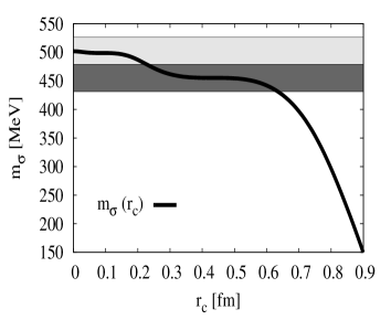
Figure 6: Short distance cut-off $r_{c}$ (in fm) dependence of the ${}^{1}S_{0}$ phase shift fitting procedure. $\chi^{2}/{\rm DOF}$ (upper panel) and $m_{\sigma}$ (lower panel). The bands represent the error estimate for two fixed cut-off values: a finite cut-off $r_{c}=0.4{\rm fm}$ and the renormalized case $r_{c}=0{\rm fm}$.

It is interesting to analyze the dependence of the fitted scalar parameters on the short distance cut-off radius, $r_{c}$. A priori we should see the $\sigma$ exchange for $r_{c}\leq 1/m_{\sigma}=0.4{\rm fm}$. From Fig. 6 we see the masses and the couplings providing an acceptable fit $\chi^{2}/{\rm DOF}<1$ for which a reliable error analysis may be undertaken. As we see this happens for $r_{c}<0.6{\rm fm}$ and two stable plateau regions yielding two potentially conflicting central $m_{\sigma}$ values. An error analysis both at a finite cut-off value $r_{c}=0.4{\rm fm}$ and the renormalized cut-off limit $r_{c}=0{\rm fm}$. gives two overlapping and hence compatible bands. This shows that in this case the data do not discriminate below $r_{c}=0.5{\rm fm}$. Much above that scale, the $\sigma$ meson becomes nearly irrelevant, as the coupling becomes rather small.

Alternatively, we may treat the cut-off itself as a fitting parameter. To avoid the large $m_{\sigma}-g_{\sigma NN}$ correlations displayed in Fig. 4 we fix the coupling constant to its central value $g_{\sigma NN}=9.1$ and get then $r_{c}=0.10^{+0.13}_{-0.07}{\rm fm}$ and $m_{\sigma}=500(3){\rm MeV}$. This shows that removing the cut-off is not only a nice theoretical requirement, but also a preferred phenomenological choice.

To analyze now the role of vector mesons we note, as already discussed in Section III.2, the redundant combination of coupling constants $g_{\omega NN}^{2}-f_{\rho NN}^{2}m_{\rho}^{2}/(2M_{N}^{2})$ which appears in the ${}^{1}S_{0}$ potential when we take $m_{\rho}=m_{\omega}$. We thus define the effective coupling $g_{\omega NN}^{*}$ defined in Eq. (41). This combination is responsible for the repulsive contribution to the potential in the ${}^{1}S_{0}$ channel. From typical values of the couplings $g_{\omega NN}=9-10.5$ and $f_{\rho NN}=15-17$ we expect $g_{\omega NN}^{*}$ to be effectively small. We show in Fig. (5) the corresponding $\chi^{2}/DOF$ as well as the readjusted scalar mass $m_{\sigma}$ and coupling $g_{\sigma NN}$ as a function of the effective combination of coupling constants, $g_{\omega NN}^{*}$. As we see, the fit is rather insensitive but actually slightly worse than without vector mesons when their contribution is repulsive. Thus, we will fix this effective coupling to zero which corresponds to take

$$g_{\omega NN}^{2}=\frac{f_{\rho NN}^{2}m_{\rho}^{2}}{2M_{N}^{2}}$$ (86)

This choice has the practical advantage of fixing $g_{\sigma NN}$ and $m_{\sigma}$ to the values provided in Eq. (84) also when the leading $N_{c}$ vector meson contributions are included. Moreover, it is also phenomenologically satisfactory as we have discussed above. In Sect. VI we will also see that deuteron or triplet ${}^{3}S_{1}-^{3}D_{1}$ do not fix the deviations from the relation given by Eq. (86).

V.4 Discussion

The linear $g_{\sigma NN}-m_{\sigma}$ correlation can be established solely by requiring that the effective range of the Nijmegen group $r_{0}=2.67{\rm fm}$ or any other be reproduced Ruiz Arriola et al. (2007). Actually, Eq. (84), yields the combination $C_{\sigma}=g_{\sigma NN}^{2}/m_{\sigma}^{2}=331(50){\rm GeV}^{-2}$ which is fixed by the effective range and not by the scattering length. This is in contrast with the resonance saturation viewpoint adopted in Ref. Epelbaum et al. (2002) where this combination fixes the scattering length.

Furthermore our calculation shows that an accurate fit without explicit contribution of the vector mesons is possible. In particular, our potential does not exhibit any repulsive region. This is in apparent contradiction with the traditional view point that the $\omega$-meson is responsible for the short range repulsion of the nuclear force.

Figure 7: Zero energy wave function for the singlet pn ${}^{1}S_{0}$ channel as a function of distance (in fm). This wave function goes asymptotically to $u_{0}(r)\to 1-r/\alpha_{0}$ with $\alpha_{0}=-23.74{\rm fm}$ the scattering length in this channel.

To understand this issue we plot in Fig. 7 the zero energy wave function obtained by integrating in with the physical scattering length $\alpha_{0}$. As we see, there appear two zeros indicating, according to the oscillation theorem, the existence of two negative energy spurious bound states. To compute such a state we solve Eq. (67) with negative energy $E_{B}=-\gamma_{B}^{2}/M$, for an exponentially decaying wave function, $u_{B}(r)\to A_{B}e^{-\gamma_{B}r}$ (normalized to one), and impose orthogonality to the zero energy state, namely

$$u_{0}u_{B}^{\prime}-u_{0}^{\prime}u_{B}\Big{|}_{r=r_{c}}=0\,,$$

from which $\gamma_{B}$ can be determined. A direct calculation yields $E_{B1}=-777{\rm MeV}$ and $A_{B1}=15.64{\rm fm}^{-1/2}$ and $E_{B2}=-11077{\rm MeV}$ and $A_{B2}=27.43{\rm fm}^{-1/2}$. If we regard the scattering amplitude as a function of energy in the complex plane, these spurious bound state energies are beyond well the maximum CM energy we want to describe in elastic NN scattering, $E_{\rm CM}\leq 175{\rm MeV}$, and so have no practical effect on the scattering region. The appearance of spurious bound states in EFT approaches are commonplace; one must check that they are beyond the considered energy range.

In order to discuss this point further we may try several ways of removing the unwanted poles and to quantify the effect on the results. Unitarity implies the usual relation between the partial wave amplitude and the phase shift

$$\left[f_{0}(p)\right]^{-1}=p\cot\delta_{0}(p)-ip$$ (88)

Actually, the contribution of a negative energy state to the s-wave scattering amplitude is a pole contribution

$$f_{0}(p)|_{B}=-\frac{A_{B}^{2}}{M}\frac{1}{E+|E_{B}|}=-\frac{A_{B}^{2}}{p^{2}+\gamma_{B}^{2}}$$ (89)

A simple way of subtracting such a bound state without spoiling unitarity and preserving the value of the amplitude at threshold $f_{0}(0)=F_{0}(0)=-\alpha_{0}$ is to modify the real part of the inverse amplitude as follows,

$$\frac{1}{F_{0}(p)}=\frac{1}{f_{0}(p)}-\frac{p^{2}}{A_{B}^{2}}\,,$$ (90)

which has no pole at $E=-|E_{B}|$, since $F_{0}(i\gamma_{B})=A_{B}^{2}/\gamma_{B}^{2}$. Using the relation between amplitude and phase shift $F_{0}(p)=1/(p\cot\Delta_{0}(p)-ip)$ we get the modified phase shift,

$$p\cot\Delta_{0}(p)=p\cot\delta_{0}(p)+\frac{p^{2}}{A_{B}^{2}}\,,$$ (91)

which corresponds to a change in the effective range

$$\Delta r_{0}|_{B}=\frac{2}{A_{B}^{2}}$$ (92)

For the values of the two spurious bound states we get $\Delta r_{0}|_{B}=0.008,0.002{\rm fm}$, a tiny amount. The change in the phase shift never exceeds $0.1^{0}$. Of course, this is not the only procedure to remove spurious bound states, but the result indicates that the effect should be small.

Another practical way to verify this issue is to study the influence of changing the cut-off $r_{c}$ from the lowest value not generating any spurious bound state and the origin, corresponding to look for $u_{0}(a)=0$. This point is clearly identified as the outer zero of the wave function, which takes place at about $a=0.5{\rm fm}$. Thus, if we choose $r_{c}=a$, there will not be any bound state. For this particular point, the orthogonality of states, Eq. (72), implies that $u_{p}(a)=0$, resembling the standard hard core picture, if we assume $u_{p}(r)=0$ for $r\leq a$. Thus, at this $r_{c}$ our method would correspond to infinite repulsion below that scale. In other words, the boundary condition does incorporate some effective repulsion which need not be necessarily visualized as a potential. The advantage of using a boundary condition is that we need not require modelling nor deep understanding on the inaccessible and unknown short distance physics.

The contribution to the effective range from the origin to the “hard core” radius $a$ is $r_{0}^{\rm in}\sim 0.04{\rm fm}$, while the change in the phase shift at the maximum energy due to the inner region $0\leq r\leq a$ is $\Delta\delta_{0}=6^{0}$ to be compared with the error estimate $\Delta\delta_{0}=0.7^{0}$ from the PWA analysis of the Nijmegen group Stoks et al. (1993) or the $\Delta\delta_{0}=2^{0}$ from the corresponding high quality potentials Stoks et al. (1994). If we identify this hard core radius to the breakdown scale of the potential, these differences might be interpreted as a systematic error of the renormalization approach for our OBE potential and, as we see, they turn out to be rather reasonable.

VI The triplet channel

VI.1 Equations and boundary conditions

The ${}^{3}S_{1}-^{3}D_{1}$ wave function in the pn CM system can be written as

$$\Psi(\vec{x}) = \frac{1}{\sqrt{4\pi}\,r}\,\Big{[}u(r)\sigma_{p}\cdot\sigma_{n}$$ (93)

$$+ \frac{w(r)}{\sqrt{8}}\left(3\sigma_{p}\cdot\hat{x}\,\sigma_{n}\cdot\hat{x}-\sigma_{p}\cdot\sigma_{n}\right)\Big{]}\chi_{pn}^{sm_{s}}$$

with the total spin $s=1$ and $m_{s}=0,\pm 1$ and $\sigma_{p}$ and $\sigma_{n}$ the Pauli matrices for the proton and the neutron respectively. The functions $u(r)$ and $w(r)$ are the reduced S- and D-wave components of the relative wave function respectively. They satisfy the coupled set of equations in the ${}^{3}S_{1}-^{3}D_{1}$ channel

$$-u^{\prime\prime}(r)+U_{{}^{3}S_{1}}(r)u(r)+U_{E_{1}}(r)w(r) = MEu(r)\,,$$

$$-w^{\prime\prime}(r)+U_{E_{1}}(r)u(r)+\left[U_{{}^{3}D_{1}}(r)+\frac{6}{r^{2}}\right]w(r) = MEw(r)\,,$$

with $U_{{}^{3}S_{1}}(r)$, $U_{E_{1}}(r)$ and $U_{{}^{3}D_{1}}(r)$ the corresponding matrix elements of the coupled channel potential

$$U_{{}^{3}S_{1}} = M(V_{C}-3W_{S})\,,$$

$$U_{E_{1}} = -6\sqrt{2}MW_{T}\,,$$

$$U_{{}^{3}D_{1}} = M(V_{C}-3W_{S}+6W_{T})\,.$$ (95)

At short distances one has the leading singularity

$$U_{{}^{3}S_{1}} = {\cal O}(r^{-1})\,,$$

$$U_{E_{1}} = -\frac{4\sqrt{2}R}{r^{3}}+{\cal O}(r^{-1})\,,$$

$$U_{{}^{3}D_{1}} = -\frac{12R}{r^{3}}+{\cal O}(r^{-1})\,.$$ (96)

where

$$\pm R=\frac{g_{\pi NN}^{2}-f_{\rho NN}^{2}}{32\pi M_{N}}$$ (97)

This is very similar to the pure OPE case treated in Ref. Pavon Valderrama and Ruiz Arriola (2005) but with the important technical difference that for $f_{\rho NN}<g_{\pi NN}$ and $f_{\rho NN}>g_{\pi NN}$ there is a turn-over of repulsive-attractive eigenchannels since the effective short distance scale $R$ changes sign. Thus, we must distinguish two different cases . At short distances we have for $g_{\pi NN}>f_{\rho NN}$ the plus sign in Eq. (97) yielding

$$u_{A}(r) = \sqrt{\frac{2}{3}}u(r)+\frac{1}{\sqrt{3}}w(r)\,,$$

$$u_{R}(r) = -\frac{1}{\sqrt{3}}u(r)+\sqrt{\frac{2}{3}}w(r)\,,$$ (98)

whereas for $g_{\pi NN}<f_{\rho NN}$ the minus sign in Eq. (97) is taken and the solutions are interchanged

$$u_{R}(r) = \sqrt{\frac{2}{3}}u(r)+\frac{1}{\sqrt{3}}w(r)\,,$$

$$u_{A}(r) = -\frac{1}{\sqrt{3}}u(r)+\sqrt{\frac{2}{3}}w(r)\,,$$ (99)

yielding an attractive singular potential $U_{A}\to-4R/r^{3}$ for $u_{A}$ and $U_{R}\to 8R/r^{3}$ for $u_{R}$, which solutions are

$$u_{R}(r) \to \left(\frac{r}{R}\right)^{3/4}\left[C_{1R}e^{+4\sqrt{2}\sqrt{\frac{R}{r}}}+C_{2R}e^{-4\sqrt{2}\sqrt{\frac{R}{r}}}\right]\,,$$

$$u_{A}(r) \to \left(\frac{r}{R}\right)^{3/4}\left[C_{1A}e^{-4i\sqrt{\frac{R}{r}}}+C_{2A}e^{4i\sqrt{\frac{R}{r}}}\right]\,.$$

The constants $C_{1R}$, $C_{2R}$, $C_{1A}$ and $C_{2A}$ depend on both $\gamma$ and $\eta$ and the OBE potential parameters. As it was discussed in Ref. Pavon Valderrama and Ruiz Arriola (2005) we must define a common domain of wave functions to define a complete solution of the Hilbert space in this ${}^{3}S_{1}-^{3}D_{1}$ channel. This is achieved taking

$$u_{R}(r) \to C_{R}(\gamma)\left(\frac{r}{R}\right)^{3/4}e^{-4\sqrt{2}\sqrt{\frac{R}{r}}}\,,$$

$$u_{A}(r) \to C_{A}(\gamma)\left(\frac{r}{R}\right)^{3/4}\sin\left[4\sqrt{\frac{R}{r}}+\varphi\right]\,.$$ (101)

Here, the short distance phase $\varphi$ is energy independent. This can be done by matching the numerical solutions to the short distance expanded ones, a cumbersome procedure in practice Pavon Valderrama and Ruiz Arriola (2005). It is far more convenient to use an equivalent short distance cut-off method with a boundary condition. Thus, at the cut-off boundary, $r=r_{c}$ we can impose a suitable regularity condition depending on the sign of $g_{\pi NN}^{2}-f_{\rho NN}^{2}$. A set of possible auxiliary boundary conditions was discussed in Ref. Pavon Valderrama and Ruiz Arriola (2005), showing that the rate of convergence was depending on the particular choice. Actually, there are infinitely many auxiliary boundary conditions which converge towards the same renormalized value, as we discuss below.

VI.2 The deuteron

In this case we have a negative energy state

$$E=-\frac{\gamma^{2}}{M}\,,$$ (102)

and we look for normalized solutions of the coupled equations (LABEL:eq:sch_coupled) and normalized to unity,

$$\int_{0}^{\infty}dr\left[u(r)^{2}+w(r)^{2}\right]=1\,,$$ (103)

which asymptotically behave as

$$u_{\gamma}(r) \to A_{S}e^{-\gamma r}\,,$$

$$w_{\gamma}(r) \to A_{S}\eta e^{-\gamma r}\left(1+\frac{3}{\gamma r}+\frac{3}{(\gamma r)^{2}}\right)\,,$$ (104)

where $A_{S}$ is the asymptotic wave function normalization and $\eta$ is the asymptotic D/S ratio. To solve this problem we introduce, as suggested in Pavon Valderrama and Ruiz Arriola (2005), the auxiliary problems

$$\begin{pmatrix}u_{S}\\ w_{S}\end{pmatrix} \to \begin{pmatrix}1\\ 0\end{pmatrix}e^{-\gamma r}\,,$$ (105)

$$\begin{pmatrix}u_{D}\\ w_{D}\end{pmatrix} \to \begin{pmatrix}0\\ 1\end{pmatrix}e^{-\gamma r}\left(1+\frac{3}{\gamma r}+\frac{3}{(\gamma r)^{2}}\right)\,,$$ (106)

which solutions depend on the deuteron binding energy through $\gamma$ and the OBE potential. Further, we can use the superposition principle of boundary conditions to write

$$u(r) = u_{S}(r)+\eta\,u_{D}(r)\,,$$

$$w(r) = w_{S}(r)+\eta\,w_{D}(r)\,.$$ (107)

The short distance regularity conditions (see below) must be imposed an a cut-off radius $r_{c}$ in order to determine the value of $\eta(r_{c})$. Then, for a given solution we compute several properties as a function of the cut-off radius, $r_{c}$. From the normalization condition, Eq. (103), in $r_{c}\leq r\leq\infty$ we get $A_{S}(r_{c})$. In this paper we also compute the matter radius,

$$r_{m}^{2}=\frac{\langle r^{2}\rangle}{4}=\frac{1}{4}\int_{r_{c}}^{\infty}r^{2}(u(r)^{2}+w(r)^{2})dr\,,$$ (108)

the quadrupole moment (without meson exchange currents)

$$Q_{d}=\frac{1}{20}\int_{r_{c}}^{\infty}r^{2}w(r)(2\sqrt{2}u(r)-w(r))dr\,,$$ (109)

the $D$-state probability

$$P_{D}=\int_{rc}^{\infty}w(r)^{2}dr\,,$$ (110)

which in the impulse aproximation and without meson exchange currents can be related to the deuteron magnetic moment. Finally, we also compute the inverse moment

$$\langle r^{-1}\rangle=\int_{r_{c}}^{\infty}r^{-1}(u(r)^{2}+w(r)^{2})dr\,,$$ (111)

which appears, e.g., in the multiple expansion of the $\pi$-deuteron scattering length.

As mentioned, there are infinitely many possible auxiliary conditions. This is an important point which we wish to illustrate. For instance, we could take

$$\sin\alpha u(r_{c})+\cos\alpha w(r_{c})=0\,,$$ (112)

where we may choose the parameter $\alpha$ arbitrarily . This is illustrated in Fig. (8). Note that despite possible wild behaviour all choices converge to the same value, although at a quite different rate. This is indeed another reason for removing the cut-off although it may be appealing and less demanding to choose one particular scheme where stability is found at the largest possible distances.

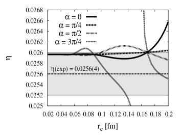
Figure 8: Short distance cut-off dependence of the asymptotic $D/S$-ratio for the case with $\pi+\sigma+\rho+\omega$. We show the dependence of the asymptotic D/S normalization $\eta$ for several choices of the arbitrary and auxiliary short distance condition $\sin\alpha u(r_{c})+\cos\alpha w(r_{c})=0$ for several values of $\alpha$.

Here we will take the smoothest auxiliary condition (labeled as BC6 in Ref. Pavon Valderrama and Ruiz Arriola (2005))

$$u^{\prime}(r_{c})-\sqrt{2}w^{\prime}(r_{c}) = 0\,,\,\,g_{\pi NN}^{2}-f_{\rho NN}^{2}>0\,,$$

$$\sqrt{2}u^{\prime}(r_{c})+w^{\prime}(r_{c}) = 0\,,\,\,g_{\pi NN}^{2}-f_{\rho NN}^{2}<0\,.$$

Clearly, for the values that we will be using the convergence is determined by the size of the short distance scale characterizing the most singular component of the potential. As we see from Eq. (97) it depends strongly on the combination $g_{\pi NN}^{2}-f_{\rho NN}^{2}$. This is an important point since the short distance cut-offs, $r_{c}$, for which convergence is achieved may change by orders of magnitude . An additional numerical problem arises due to undesired amplification of the short distance growing exponential, setting some limitations to the numerics due to roundoff errors. In all our calculations we have payed particular attention to these delicate issues.

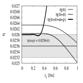
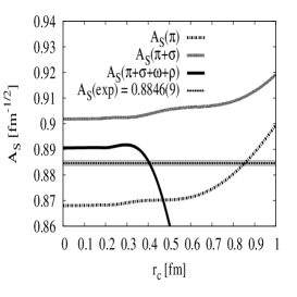
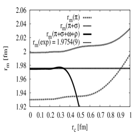
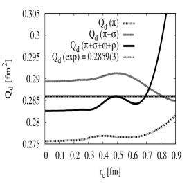
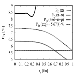
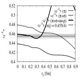
Figure 9: Short distance cut-off dependence of deuteron properties for the cases with $\pi$, $\pi+\sigma$ and $\pi+\sigma+\rho+\omega$. We show the dependence of the asymptotic D/S normalization $\eta$ (upper left panel), the S-wave normalization $A_{S}$ (in ${\rm fm}^{-1/2}$, upper middle panel), the matter radius $r_{m}$ (in ${\rm fm}$, upper right panel), the quadrupole moment $Q_{d}$ (in ${\rm fm}^{2}$, lower left panel), the $D$-state probability (lower middle panel) and the inverse radius $\langle r^{-1}\rangle$ (in ${\rm fm}^{-1}$ lower right panel). Experimental or recommended values can be traced from Ref. de Swart et al. (1995).

The cut-off dependence of these observables is shown in Fig. 9, for the case of $\pi$ only (Ref. Pavon Valderrama and Ruiz Arriola (2005)), $\pi+\sigma$ and $\pi+\sigma+\rho+\omega$ and as we see good convergence can be achieved as $r_{c}\to 0$. As already mentioned, the rate of convergence depends on the scale of the singularity.

Figure 10: Deuteron wave functions, u (left) and w (right), as a function of the distance (in fm) in the OBE. We show $1\pi$, $1\pi+1\sigma$ and $\pi+\sigma+\rho+\omega$ compared to the Nijmegen II wave functions Stoks et al. (1994). The asymptotic normalization $u\to e^{-\gamma r}$ has been adopted and the asymptotic D/S ratio is obtained to be $\eta_{\pi}=0.2633$ and $\eta_{\pi\sigma\omega\rho}=0.2597$ (see table 2).

The resulting coordinate space deuteron wave functions, $u$ and $w$, are depicted in Fig. 10 for the case of $\pi$ only (Ref. Pavon Valderrama and Ruiz Arriola (2005)), $\pi+\sigma$ and $\pi+\sigma+\rho+\omega$ and compared to the wave functions of the high quality Nijmegen potential Stoks et al. (1994). As we see, after inclusion of the scalar and vector mesons, the agreement is quite remarkable in the region above $1.4-1.8{\rm fm}$, their declared range of validity. Similarly to the singlet case, we observe oscillations in the region below 1 fm. The first node is allowed since we are dealing with a bound state, the second node occurs already below $0.5{\rm fm}$ indicating, similarly to the ${}^{1}S_{0}$ channel, the appearance of infinitely many spurious bound states, as we see from the short distance oscillatory behaviour of the wave function, Eq. (101). To compute such states we proceed similarly to the singlet channel. We solve Eq. (LABEL:eq:sch_coupled) with negative energy $E_{B}=-\gamma_{B}^{2}/M$, the asymptotic behaviour in Eq. (104) and impose the regularity conditions, Eq (LABEL:eq:bc6), as well as orthogonality to the deuteron state, namely

$$u_{\gamma}u_{B}^{\prime}-u_{\gamma}^{\prime}u_{B}+w_{\gamma}w_{B}^{\prime}-w_{\gamma}^{\prime}w_{B}\Big{|}_{r=r_{c}}=0\,,$$ (114)

from which $\gamma_{B}$ can be determined. For instance, for the scalar parameters in Eq. (84) and $f_{\rho NN}=15.5$ we identify the first spurious bound state $(u_{B1},w_{B1})$ having one node less than the deuteron wave functions $(u_{d},w_{d})$ taking place at $\gamma_{B1}=3.438{\rm fm}^{-1}$. The corresponding energy is $E_{B1}=-\gamma_{B1}^{2}/M=-490{\rm MeV}$, S-wave normalization $A_{B1}=13.58{\rm fm}^{-1/2}$ matter radius $r_{B1}=0.49{\rm fm}$ and asymptotic D/S ratio $\eta_{B1}=0.1656$. This state is clearly beyond the range of applicability of the present framework. Subtracting this pole to the ${}^{3}S_{1}$ amplitude would result, according to Eq. (92), in $\Delta r_{0}=0.01{\rm fm}$. The next spurious state has $E_{B2}<-18{\rm GeV}$!!. Note that if the scale where the second unphysical node takes place was to be interpreted as a (“hard core”) breakdown distance scale of our approach for the deuteron, it is certainly beyond the accessible region at the maximal energy in elastic NN scattering. This issue is relevant for the calculation of phase shifts where such oscillations also occur. The variation of the observables from this breakdown scale to the origin, could be interpreted as a source of systematic error coming from the fact that there is only one bound state and not infinitely many. As we see from Fig. 9 the effect is indeed small.

Numerical results for renormalized quantities can be looked up in Table 2. As we see, the inclusion of $\sigma$ provides some overall improvement while $\rho$ and $\omega$ yield a fairly accurate description of the deuteron for the choice $f_{\rho NN}=15.5$ and $g_{\omega NN}=9$ (this latter value complies to the SU(3) relation $g_{\omega NN}=3g_{\rho NN}$ when $g_{\rho NN}\sim 2.9$).

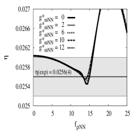
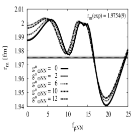
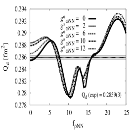
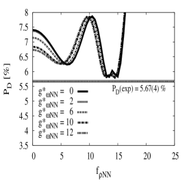
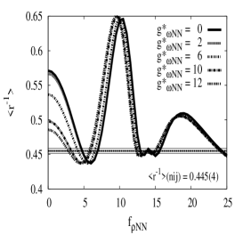
Figure 11: Dependence of the deuteron observables as a function of $f_{\rho NN}$ for several values of the the effective coupling constant $g_{\omega NN}^{*}=\sqrt{g_{\omega NN}^{2}-f_{\rho NN}^{2}m_{\rho}^{2}/2M_{N}^{2}}$. $g_{\sigma NN}$ and $m_{\sigma}$ are always readjusted to fit the ${}^{1}S_{0}$ phase shift. We show the dependence of the asymptotic D/S normalization $\eta$ (upper left panel), the S-wave normalization $A_{S}$ (in ${\rm fm}^{-1/2}$, upper middle panel), the matter radius $r_{m}$ (in ${\rm fm}$, upper right panel), the quadrupole moment $Q_{d}$ (in ${\rm fm}^{2}$, lower left panel), the $D$-state probability (lower middle panel) and the inverse radius $\langle r^{-1}\rangle$ (in ${\rm fm}^{-1}$ lower right panel). The leading $N_{c}$ contributions to the OBE ($\sigma+\pi+\rho+\omega$) potential are considered. Experimental or recommended values can be traced from Ref. de Swart et al. (1995).

Table 2: Deuteron properties and low energy parameters in the ${}^{3}S_{1}-^{3}D_{1}$ channel for OBE potentials including $\pi$, $\pi+\sigma$, $\pi+\sigma+\rho+\omega$. We use the non-relativistic relation $\gamma=\sqrt{2\mu_{np}B}$ with $B=2.224575(9)$ and take $m=138.03{\rm MeV}$, and $g_{\pi NN}=13.1083$ de Swart et al. (1997). From a fit to the ${}^{1}S_{0}$ channel we have $m_{\sigma}=501{\rm MeV}$ and $g_{\sigma NN}=9.1$. The simplifying relation $g_{\omega NN}=f_{\rho NN}m_{\rho}/\sqrt{2}M_{N}$ is used throughout. $\pi\sigma\rho\omega$ corresponds to take $f_{\rho NN}=15.5$ and $g_{\omega NN}=9.857$ while $\pi\sigma\rho\omega^{*}$ corresponds to take $f_{\rho NN}=17.0$ and $g_{\omega NN}=10.147$

	$\gamma({\rm fm}^{-1})$	$\eta$	$A_{S}({\rm fm}^{-1/2})$	$r_{m}({\rm fm})$	$Q_{d}({\rm fm}^{2})$	$P_{D}$	$\langle r^{-1}\rangle$	$\alpha_{0}({\rm fm})$	$\alpha_{02}({\rm fm}^{3})$	$\alpha_{2}({\rm fm}^{5})$	$r_{0}({\rm fm})$
$\pi$	Input	0.02633	0.8681	1.9351	0.2762	7.88%	0.476	5.335	1.673	6.169	1.638
$\pi\sigma$	Input	0.02599	0.9054	2.0098	0.2910	6.23%	0.432	5.335	1.673	6.169	1.638
$\pi\sigma\rho\omega$	Input	0.02597	0.8902	1.9773	0.2819	7.22%	0.491	5.444	1.745	6.679	1.788
$\pi\sigma\rho\omega$∗	Input	0.02625	0.8846	1.9659	0.2821	9.09%	0.497	5.415	1.746	6.709	1.748
NijmII	Input	0.02521	0.8845(8)	1.9675	0.2707	5.635%	0.4502	5.418	1.647	6.505	1.753
Reid93	Input	0.02514	0.8845(8)	1.9686	0.2703	5.699%	0.4515	5.422	1.645	6.453	1.755
Exp.	0.231605	0.0256(4)	0.8846(9)	1.9754(9)	0.2859(3)	5.67(4)		5.419(7)			1.753(8)

We show in Fig. (11) the dependence of several properties when both the vector mesons $\rho$ and $\omega$ are simultaneosuly considered. In Fig. 11 we plot the dependendence of (renormalized) deuteron properties as a function of $f_{\rho NN}$ for several values of the effective coupling constant $g_{\omega NN}^{*}=\sqrt{g_{\omega NN}^{2}-f_{\rho NN}^{2}m_{\rho}^{2}/2M_{N}^{2}}$ featuring the strong correlation in the ${}^{1}S_{0}$ channel pointed out in Section V. The scalar coupling $g_{\sigma NN}$ and scalar mass $m_{\sigma}$ are always readjusted to fit the ${}^{1}S_{0}$ phase shift. As we see, for the asymptotic D/S ratio, $\eta$, there is a wide range of possible values within the experimental uncertainties but we obtain the bounds $f_{\rho NN}\leq 15$ and $g_{\omega NN}\leq 15$. It is amazing that the value of the tensor-$\rho$ coupling is so well determined to be $f_{\rho NN}\sim 16-17$ and corresponds to the strong $\kappa_{\rho}$ situation described by Machleidt and Brown Brown and Machleidt (1994). Note that results depend in a moderate fashion on $f_{\rho NN}$ for not too large values, as one would expect from the short range of the $\rho-$meson.

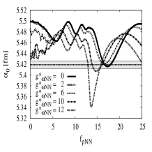
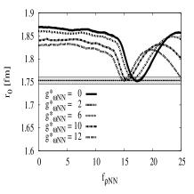
Figure 12: Dependendence of the low energy parameters as a function of $f_{\rho NN}$ for several values of the the effective coupling constant $g_{\omega NN}^{*}=\sqrt{g_{\omega NN}^{2}-f_{\rho NN}^{2}m_{\rho}^{2}/2M_{N}^{2}}$. $g_{\sigma NN}$ and $m_{\sigma}$ are always readjusted to fit the ${}^{1}S_{0}$ phase shift. We show the dependence of the ${}^{3}S_{1}$ scattering length $\alpha_{0}$ (in fm) and effective range $r_{0}$ (in fm) as well as $\alpha_{02}$ (in ${\rm fm}^{3}$) and $\alpha_{2}$ (in ${\rm fm}^{5}$) compared to the experimental values or the Nijm2 and Reid93 potentials (horizontal straight lines) The leading $N_{c}$ contributions to the OBE ($\sigma+\pi+\rho+\omega$) potential are considered.

VI.3 Zero energy

At zero energy, the asymptotic solutions to the coupled equations (LABEL:eq:sch_coupled) are given by

$$u_{0,\alpha}(r) \to 1-\frac{r}{\alpha_{0}}\,,$$

$$w_{0,\alpha}(r) \to \frac{3\alpha_{02}}{\alpha_{0}r^{2}}\,,$$

$$u_{0,\beta}(r) \to \frac{r}{\alpha_{0}}\,,$$

$$w_{0,\beta}(r) \to \left(\frac{\alpha_{2}}{\alpha_{02}}-\frac{\alpha_{02}}{\alpha_{0}}\right)\frac{3}{r^{2}}-\frac{r^{3}}{15\alpha_{02}}\,,$$ (115)

where $\alpha_{0}$, $\alpha_{2}$ and $\alpha_{02}$ are low energy parameters obtained from the phase shifts (see Sect. VI.4). Using these zero energy solutions one can determine the effective range. The ${}^{3}S_{1}$ effective range parameter is given by

$$r_{0} = 2\int_{0}^{\infty}\left[\left(1-\frac{r}{\alpha_{0}}\right)^{2}-u_{0,\alpha}(r)^{2}-w_{0,\alpha}(r)^{2}\right]dr\,.$$

(116)

Using the superposition principle of boundary conditions we may write the solutions as

$$u_{0,\alpha}(r) = u_{1}(r)-\frac{1}{\alpha_{0}}u_{2}(r)+\frac{3\alpha_{02}}{\alpha_{0}}u_{3}(r)\,,$$

$$w_{0,\alpha}(r) = w_{1}(r)-\frac{1}{\alpha_{0}}w_{2}(r)+\frac{3\alpha_{02}}{\alpha_{0}}w_{3}(r)\,,$$

$$u_{0,\beta}(r) = \frac{1}{\alpha_{0}}u_{2}(r)+\left(\frac{3\alpha_{2}}{\alpha_{02}}-\frac{3\alpha_{02}}{\alpha_{0}}\right)u_{3}(r)-\frac{1}{15\alpha_{02}}u_{4}(r)\,,$$

$$w_{0,\beta}(r) = \frac{1}{\alpha_{0}}w_{2}(r)+\left(\frac{3\alpha_{2}}{\alpha_{02}}-\frac{3\alpha_{02}}{\alpha_{0}}\right)w_{3}(r)-\frac{1}{15\alpha_{02}}w_{4}(r)\,,$$

where the functions $u_{1,2,3,4}$ and $w_{1,2,3,4}$ are independent on $\alpha_{0}$, $\alpha_{02}$ and $\alpha_{2}$ and fulfill suitable boundary conditions. The orthogonality constraints for the $\alpha$ and $\beta$ states read in this case

$$u_{\gamma}u_{0,\alpha}^{\prime}-u_{\gamma}^{\prime}u_{0,\alpha}+w_{\gamma}w_{0,\alpha}^{\prime}-w_{\gamma}^{\prime}u_{0,\alpha}\Big{|}_{r=r_{c}} = 0$$

$$u_{\gamma}u_{0,\beta}^{\prime}-u_{\gamma}^{\prime}u_{0,\beta}+w_{\gamma}w_{0,\beta}^{\prime}-w_{\gamma}^{\prime}u_{0,\beta}\Big{|}_{r=r_{c}} = 0$$

A further condition which should be satisfied is the $\alpha-\beta$ orthogonality

$$u_{0,\alpha}u_{0,\beta}^{\prime}-u_{0,\alpha}^{\prime}u_{0,\beta}+w_{0,\alpha}w_{0,\beta}^{\prime}-w_{0,\alpha}^{\prime}u_{0,\beta}\Big{|}_{r=r_{c}} = 0$$

as well as the short distance regularity conditions, Eq. (LABEL:eq:bc6). In all we have an over-determined system with 5 equations and three unknowns $\alpha_{02}$, $\alpha_{2}$ and $\alpha_{0}$. Solving the equations in triplets we have checked the numerical compatibility at the $0.01\%$ level for the shortest cut-offs, $r_{c}\sim 0.02{\rm fm}$ typically used. Using the superposition principle decomposition of the bound state, Eq. (107), and for the zero energy states, Eq. (LABEL:eq:sup_zero), one can make the orthogonality relations explicit in $\alpha_{0}$, $\alpha_{02}$, $\alpha_{2}$. The values of $\alpha_{02}$ and $\alpha_{2}$ are not so well known although they have been determined from potential models in Ref. Pavon Valderrama and Arriola (2005).

In Fig. 12 we show the dependence of the low energy parameters of the leading $N_{c}$ contributions to the OBE ($\sigma+\pi+\rho+\omega$) potential as a function of $f_{\rho NN}$ for several values of the the effective coupling constant $g_{\omega NN}^{*}=\sqrt{g_{\omega NN}^{2}-f_{\rho NN}^{2}m_{\rho}^{2}/2M_{N}^{2}}$ being $g_{\sigma NN}$ and $m_{\sigma}$ always readjusted to fit the ${}^{1}S_{0}$ phase shift. Similarly to the deuteron case we observe stronger dependence on $f_{\rho NN}$ and a relative insensitivity on the effective coupling $g_{\omega NN}^{*}$. We remind that along any of these curves the ${}^{1}S_{0}$ phase shift is well reproduced with an acceptable $\chi^{2}/{\rm DOF}<1$. As we see, the values $f_{\rho NN}=17.0$ and $g_{\omega NN}^{*}=0$ reproduce quite well the low energy parameters, corresponding to the reasonable $g_{\omega NN}=10.4$.

Numerical results for the low energy parameters are shown in Table 2. Again, the inclusion of $\sigma$ provides some overall improvement while $\rho$ and $\omega$ yield a better description of the deuteron for the choice $f_{\rho NN}=15.5$ and $g_{\omega NN}=9.0$. There is nonetheless a small mismatch to the experimental or recommended potential values when the zero energy wave functions are obtained from the orthogonality relations to the deuteron, Eq. (LABEL:eq:orth_triplet). As one can see further improvement is obtained when $f_{\rho NN}=17.0$ and $g_{\omega NN}=10.3$. In this case we get a SU(3) violation; $g_{\omega NN}=3.5g_{\rho NN}$, which actually agrees with the expectations from radiative decays $\omega\to e^{+}e^{-}$ and $\rho\to e^{+}e^{-}$ (see e.g. Dumbrajs et al. (1983)).

Figure 13: Convergence of the np Spin Triplet Eigen phase shifts for the total angular momentum $j=1$ as a function of the short distance cut-off radius $r_{c}$ (in fm) for several fixed values of the CM momentum $p=100,200,300$ and $400{\rm MeV}$.

Figure 14: np Spin Triplet Eigen phase shifts for the total angular momentum $j=1$ as a function of as a function of the CM momentum. We show $\pi$, $\pi+\sigma$ and $\pi+\sigma+\rho+\omega$ compared to an average of the Nijmegen partial wave analysis and high quality potential models Stoks et al. (1993, 1994). We take $(f_{\rho NN},g_{\omega NN})=(15.5,9.857)$, $(f_{\rho NN},g_{\omega NN})=(17.0,10.147)$, .

VI.4 Phase shifts

Finally, in the case of positive energy we consider Eq. (LABEL:eq:sch_coupled) with

$$E=\frac{p^{2}}{M}\,,$$ (120)

with $p$ the corresponding CM momentum. We solve Eq. (LABEL:eq:sch_coupled) for the $\alpha$ and $\beta$ positive energy scattering states and choose the asymptotic normalization

$$u_{k,\alpha}(r) \to \frac{\cos\epsilon}{\sin\delta_{1}}\Big{(}\hat{j}_{0}(kr)\cos\delta_{1}-\hat{y}_{0}(kr)\sin\delta_{1}\Big{)}\,,$$

$$w_{k,\alpha}(r) \to \frac{\sin\epsilon}{\sin\delta_{1}}\Big{(}\hat{j}_{2}(kr)\cos\delta_{1}-\hat{y}_{2}(kr)\sin\delta_{1}\Big{)}\,,$$

$$u_{k,\beta}(r) \to -\frac{1}{\sin\delta_{1}}\Big{(}\hat{j}_{0}(kr)\cos\delta_{2}-\hat{y}_{0}(kr)\sin\delta_{2}\Big{)}\,,$$

$$w_{k,\beta}(r) \to \frac{\tan\epsilon}{\sin\delta_{1}}\Big{(}\hat{j}_{2}(kr)\cos\delta_{2}-\hat{y}_{2}(kr)\sin\delta_{2}\Big{)}\,,$$

where $\hat{j}_{l}(x)=xj_{l}(x)$ and $\hat{y}_{l}(x)=xy_{l}(x)$ are the reduced spherical Bessel functions and $\delta_{1}$ and $\delta_{2}$ are the eigen-phases in the ${}^{3}S_{1}$ and ${}^{3}D_{1}$ channels, and $\epsilon$ is the mixing angle $E_{1}$. To carry out the renormalization program, we use the superposition principle of boundary conditions which makes the discussion more transparent. Let us define the four auxiliary problems

$$\begin{pmatrix}u_{k,1}\\ w_{k,1}\end{pmatrix}\to\begin{pmatrix}\hat{j}_{0}(kr)\\ 0\end{pmatrix}\,,\qquad\begin{pmatrix}u_{k,2}\\ w_{k,2}\end{pmatrix}\to\begin{pmatrix}\hat{y}_{0}(kr)\\ 0\end{pmatrix}\,,\qquad\begin{pmatrix}u_{k,3}\\ w_{k,3}\end{pmatrix}\to\begin{pmatrix}0\\ \hat{j}_{2}(kr)\end{pmatrix}\,,\qquad\begin{pmatrix}u_{k,4}\\ w_{k,4}\end{pmatrix}\to\begin{pmatrix}0\\ \hat{y}_{2}(kr)\end{pmatrix}\,,$$ (122)

which depend solely on the potential and can be obtained by integrating in. Thus, the general solution satisfying the $\alpha$ and $\beta$ asymptotic conditions can be written as

$$u_{k,\alpha}(r)=\sum_{i=1}^{4}c_{i,\alpha}u_{k,i}(r)\,,\quad w_{k,\alpha}(r)=\sum_{i=1}^{4}c_{i,\alpha}w_{k,i}(r)\,,\quad u_{k,\beta}(r)=\sum_{i=1}^{4}c_{i,\beta}u_{k,i}(r)\,,\quad w_{k,\beta}(r)=\sum_{i=1}^{4}c_{i,\beta}w_{k,i}(r)\,.$$ (123)

Fixing the constants to the asymptotic conditions Eq. (LABEL:eq:phase_triplet) we get

$$u_{k,\alpha}(r) = \frac{\cos\epsilon}{\sin\delta_{\alpha}}\Big{(}u_{1}(r)\cos\delta_{\alpha}-u_{2}(r)\sin\delta_{\alpha}\Big{)}\,$$

$$+ \frac{\sin\epsilon}{\sin\delta_{\alpha}}\Big{(}\cos\delta_{\alpha}u_{3}(r)-u_{4}(r)\sin\delta_{\alpha}\Big{)}\,,$$

$$w_{k,\alpha}(r) = \frac{\cos\epsilon}{\sin\delta_{\alpha}}\Big{(}w_{1}(r)\cos\delta_{\alpha}-w_{2}(r)\sin\delta_{\alpha}\Big{)}\,$$

$$+ \frac{\sin\epsilon}{\sin\delta_{\alpha}}\Big{(}\cos\delta_{\alpha}w_{3}(r)-w_{4}(r)\sin\delta_{\alpha}\Big{)}\,,$$

$$u_{k,\beta}(r) = \frac{1}{\sin\delta_{\alpha}}\Big{(}u_{1}(r)\cos\delta_{\beta}-u_{2}(r)\sin\delta_{\beta}\Big{)}\,$$

$$- \frac{\tan\epsilon}{\sin\delta_{\alpha}}\Big{(}\cos\delta_{\beta}u_{3}(r)-u_{4}(r)\sin\delta_{\beta}\Big{)}\,,$$

$$w_{k,\beta}(r) = \frac{1}{\sin\delta_{\alpha}}\Big{(}w_{1}(r)\cos\delta_{\beta}-w_{2}(r)\sin\delta_{\beta}\Big{)}\,$$

$$- \frac{\tan\epsilon}{\sin\delta_{\alpha}}\Big{(}\cos\delta_{\beta}w_{3}(r)-w_{4}(r)\sin\delta_{\beta}\Big{)}\,.$$

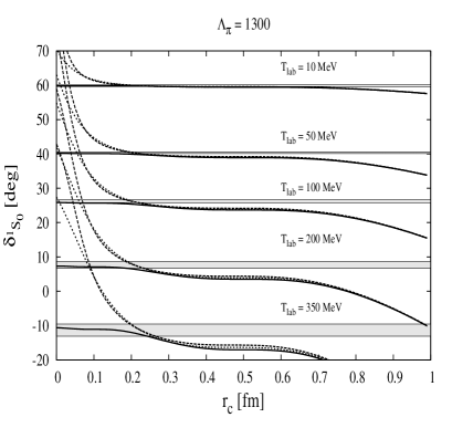
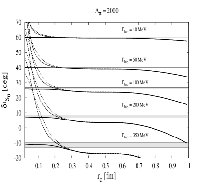
Figure 15: Convergence of the np Spin Singlet ${}^{1}S_{0}$ phase shift (in degrees) as a function of the short distance cut-off radius $r_{c}$ (in fm) for several fixed values of the LAB energy when the scattering length $\alpha_{0}=-23.74{\rm fm}$ is also fixed. We compare the purely renormalized case with no form factors (solid line) with the renormalization also including the exponential (dotted line) and monopole (dashed line) form factors and for the cut-off values $\Lambda_{\pi NN}=1300{\rm MeV}$ (left panel) and $\Lambda_{\pi NN}=2000{\rm MeV}$ (right panel), all others fixed to $\Lambda_{\sigma NN}=\Lambda_{\rho NN}=\Lambda_{\omega NN}=2{\rm GeV}$. We also add the error bands related to the Nijmegen PWA and high quality potentials Stoks et al. (1993, 1994). All other meson parameters in the OBE potential are kept the same.

In the low energy limit $\epsilon\to-\alpha_{02}k^{3}$ $\delta_{\alpha}\to-\alpha_{0}k$ and $\delta_{\beta}\to-(\alpha_{2}-\alpha_{02}^{2}/\alpha_{0})k^{5}$ and the zero energy solutions discussed in Sec. VI.3 are reproduced. The use of the superposition principle for boundary conditions as well as the orthogonality constraints to the deuteron wave analogous to Eq. (72) yields

$$u_{\gamma}u_{k,\alpha}^{\prime}-u_{\gamma}^{\prime}u_{k,\alpha}+w_{\gamma}w_{k,\alpha}^{\prime}-w_{\gamma}^{\prime}u_{k,\alpha}\Big{|}_{r=r_{c}} = 0$$

$$u_{\gamma}u_{k,\beta}^{\prime}-u_{\gamma}^{\prime}u_{k,\beta}+w_{\gamma}w_{k,\beta}^{\prime}-w_{\gamma}^{\prime}u_{k,\beta}\Big{|}_{r=r_{c}} = 0$$

which together with the short distance regularity conditions, Eq. (LABEL:eq:bc6) allow us to deduce the corresponding ${}^{3}S_{1}-^{3}D_{1}$ phase-shifts. A further condition is the $\alpha-\beta$ orthogonality

$$u_{k,\alpha}u_{k,\beta}^{\prime}-u_{k,\alpha}^{\prime}u_{k,\beta}+w_{k,\alpha}w_{k,\beta}^{\prime}-w_{k,\alpha}^{\prime}u_{k,\beta}\Big{|}_{r=r_{c}} = 0$$

In all we have an over-determined system with 5 equations and three unknowns. We have checked that almost any choice yields equivalent results with an accuracy of $0.001^{o}$ for the highest CM momenta and the shortest cut-off, $r_{c}\sim 0.02{\rm fm}$.

Table 3: Fits to the Renormalized ${}^{1}S_{0}$ phase shift of the Nijmegen group Stoks et al. (1994) using the OBE potential without or with strong exponential and monopole form factor. We fix $\alpha_{0}=-23.74{\rm fm}$ and take $m=138.03{\rm MeV}$, and $g_{\pi NN}=13.1083$ de Swart et al. (1997) and $m_{\rho}=m_{\omega}=770{\rm MeV}$ and fit $m_{\sigma}$, $g_{\sigma NN}$ and fix $g_{\omega NN}^{*}=0$. We use $\Lambda_{\pi NN}=1300{\rm MeV}$ and $\Lambda_{\sigma NN}=\Lambda_{\rho NN}=\Lambda_{\omega NN}=2000{\rm MeV}$. $E_{B}$ represents the energy of the (spurious) bound state when it does exist.

	$r_{c}({\rm fm})$	$m_{\sigma}({\rm MeV})$	$g_{\sigma NN}$	$g_{\omega NN}^{*}$	$\chi^{2}/DOF$	$\alpha_{0}({\rm fm})$	$r_{0}({\rm fm})$	$E_{B}({\rm MeV})$
$\Gamma(q^{2})=1$	0	501(25)	9(1)	0(3)	0.12	Input	2.695	-777
$\Gamma(q^{2})=\Gamma^{\rm exp}(q^{2})$	0	526(20)	10.4(8)	0(3)	0.19	Input	2.692	-790
$\Gamma(q^{2})=\Gamma^{\rm exp}(q^{2})$	0.1	523(27)	10.2(1.1)	0(3)	0.18	Input	2.491	-834
$\Gamma(q^{2})=\Gamma^{\rm mon}(q^{2})$	0	532(20)	10.7(7)	0(3)	0.20	Input	2.691	-796
$\Gamma(q^{2})=\Gamma^{\rm mon}(q^{2})$	0.1	528(28)	10.5(1.1)	0(3)	0.19	Input	2.490	-853

As we have mentioned already, the numerical solution of the problem requires taking care of spurious amplification of the undesired growing exponential at any step of the calculation. The situation is aggravated by the fact that for the phase shifts the maximum momentum $p=400{\rm MeV}$ explores the region around $0.1-0.5{\rm fm}$, so it is important to make sure that we do not see cut-off effects in this region. To provide a handle on the numerical uncertainties we show in Fig. (13) the results for the phase shifts $\delta_{1}$, $\delta_{2}$ and $\epsilon$ as a function of the cut-off radius, $r_{c}$ and for several fixed CM pn momenta, $p=100,200,300,400{\rm MeV}$. As we see, there appear clear plateaus between $0.1-0.2{\rm fm}$ which somewhat steadily shrink when the momentum is increased. Note that these values of the short distance cut-off translates into a CM momentum space cut-off range $\Lambda=\pi/(2r_{c})=1.5-3{\rm GeV}$.

The results for the ${}^{3}S_{1}-^{3}D_{1}$ phase shifts as a function of the CM momentum are depicted in Fig. 14 for $\pi$, $\pi+\sigma$ and $\pi+\sigma+\rho+\omega$ and compared to the Nijmegen analysis Stoks et al. (1993, 1994). We use $g_{\sigma NN}=9.1$, $m_{\sigma}=501{\rm MeV}$ and when vector mesons are included we take $f_{\rho NN}=15.5$ and $g_{\omega NN}=9$ or $f_{\rho NN}=17.0$ and $g_{\omega NN}=10.147$ corresponding to Sets $\pi\sigma\rho\omega$ and $\pi\sigma\rho\omega^{*}$ in Table 2 respectively. On a first sight we see an obvious improvement in both the ${}^{3}S_{1}$ and ${}^{3}D_{1}$ phases and not so much in the mixing angle $E_{1}$ as compared to the simple OPE case. One should note, however, that besides describing by construction the single phase shift ${}^{1}S_{0}$ (see Fig. (4) ) we also improve on the deuteron (see Table 2). Obviously, it would be possible to provide a better description of triplet phase shifts, however, at the expense of worsening the deuteron properties and the singlet channel. Clearly, there is room for improvement, and our results call for consideration of sub-leading large $N_{c}$ corrections in the OBE potential. This would incorporate, the relative to leading $1/N_{c}^{2}$ relativistic corrections, spin-orbit effects, finite meson widths, non-localities, etc.

VII Influence of Strong form factors in the renormalization process

Given the reasonable phenomenological success of the renormalization approach one may naturally wonder what would be the effect of the form factors in our calculation. In this section we discuss the influence of strong form factors in the calculated properties on top of the renormalization process. Our main quest is to find out whether they lead to observable physical effects after renormalization. An equivalent way of posing the question is to determine whether finite nucleon size effects can be disentangled explicitly in NN scattering in the elastic region.

To analyze this important issue in detail, in Fig. 15 we show the phase shift in the ${}^{1}S_{0}$ channel for fixed LAB energy values as a function of the short distance cut-off radius $r_{c}$ when the scattering length is fixed to its experimental value, $\alpha_{0}=-23.74{\rm fm}$ as we explained in Section  V. We use the same parameters as for the renormalized solution without vertex function, for several fixed values of the LAB energy and for the cut-off values $\Lambda_{\pi NN}=1300{\rm MeV}$ and $\Lambda_{\pi NN}=2000{\rm MeV}$, all others fixed to $\Lambda_{\sigma NN}=\Lambda_{\rho NN}=\Lambda_{\omega NN}=2{\rm GeV}$. As one clearly sees strong form factors are invisible for $r_{c}>0.3{\rm fm}$. For lower values of the short distance cut-off $r_{c}$ both monopole and exponential form factors agree with each other but deviate strongly from the Nijmegen database. Note that the lines should be supplemented with estimates of theoretical errors, not shown to avoid cluttering of the plot. When those errors are included the Nijmegen data are basically compatible with the theoretical curves in the flat preasymptotic region around $0.3-0.5{\rm fm}$ (see also the discussion around Fig. 6).

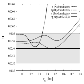
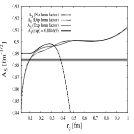
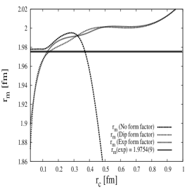
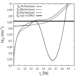
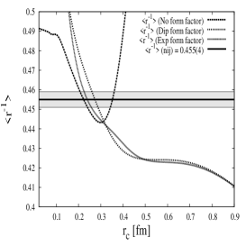
Figure 16: Short distance cut-off $r_{c}$ dependence of deuteron properties for the $\pi\sigma\rho\omega$ case (see table 2). We compare the purely renormalized calculation with the cases for both exponential, Eq. (31), and monopole Eq. (30) form factors taking $\Lambda_{\pi NN}=1300{\rm MeV}$, all other cut-offs being kept to $\Lambda_{\sigma NN}=\Lambda_{\rho NN}=\Lambda_{\omega NN}=2000{\rm MeV}$. We show the dependence of the asymptotic D/S normalization $\eta$ (upper left panel), the S-wave normalization $A_{S}$ (in ${\rm fm}^{-1/2}$, upper middle panel), the matter radius $r_{m}$ (in ${\rm fm}$, upper right panel), the quadrupole moment $Q_{d}$ (in ${\rm fm}^{2}$, lower left panel), the $D$-state probability (lower middle panel) and the inverse radius $\langle r^{-1}\rangle$ (in ${\rm fm}^{-1}$ lower right panel). Experimental or recommended values can be traced from Ref. de Swart et al. (1995).

Of course, one may attribute the discrepancy to the choice of parameters, which have been chosen to fit the renormalized solution without form factors. A somewhat complementary way of seeing this is by refitting the parameters using both exponential and monopole vertex functions but fixing by construction the scattering length $\alpha_{0}$. The results for $\Lambda_{\pi NN}=1.3{\rm GeV}$ and $\Lambda_{\sigma NN}=\Lambda_{\rho NN}=\Lambda_{\omega NN}=2{\rm GeV}$ are displayed in Table 3. As we see, the parameters change almost within the uncertainties, showing the marginal effect of the vertex functions after renormalization. Due to the presence of non-linear correlations, difficult to handle by standard means, we have fixed $g_{\omega NN}^{*}$ to its minimum value (compatible with zero) and estimated its error by varying it independently from its mean value to values still giving an acceptable fit, yielding $g_{\omega NN}^{*}=0(3)$. We also show the effect of the short distance cut-off $r_{c}$ which, as we see, is rather small. Overall, these results provide a further confirmation of our naive expectations; nucleon finite size effects and vector mesons do not provide the bulk in NN scattering in central waves, and actually cannot be clearly resolved. Of course, this should be checked in higher partial waves, but those are expected in fact to be less sensitive to short distances.

Finally, in Fig. 16 the influence of the vertex functions is analyzed for some of the computed deuteron properties. As we see there is a fair coincidence of the purely renormalized solution with no form factors with the equally renormalized solution including the form factors in the potential in the region around $r_{c}\sim 0.3-0.6{\rm fm}$. The deviation below 0.3 fm signals the onset of the irregular $D$-wave solution, which behaves as $w(r)\sim r^{-2}$ at small distances and hence yields eventually a divergent result. Note that in order to have a smooth behaviour at short distances when renormalization is over-imposed to the potential with form factors we should choose the regular D-wave solution $w(r)\sim r^{3}$ but then the potential parameters, either couplings or form factor cut-off parameters should also be fine-tuned.

While it is fairly clear that vertex functions do exist and are of fundamental importance, it is also true that they start playing a role as soon as the probing wavelength resolves the finite nucleon size. Our calculations suggest on a quantitative level that provided the NN scattering data are properly described with form factors, they will be effectively irrelevant under the renormalization process, and for CM momenta below $400{\rm MeV}$, vertex functions are expected to play a marginal role.

VIII Conclusions and Outlook

In the present paper we have analyzed the OBE potential from a renormalization point of view. As we have shown, the meson-nucleon Lagrangean does not predict the S-matrix beyond perturbation theory. The non-perturbative nature of low partial waves and the deuteron in the NN problem suggests resuming OBE diagrams by extracting the corresponding potential. The OBE potential, however, presents short distance divergences which make the solution of the corresponding Schrödinger equation ambiguous. The traditional remedy for this problem has been the inclusion of phenomenological form factors which parameterize the vertex functions in the meson exchange picture. We have shown that the meson exchange potential with form factors generates spurious deeply bound states for natural values of the coupling constants. The price to remove those is to fine tune the potential at all distances, and in particular at short distances. Thus, while it is claimed that vertex functions implement the finite nucleon size, it is very difficult to disentangle this from meson dressing and many other effects where the meson theory does not hold.

The renormalization approach suggests that extracting this detailed short distance information may in fact be unnecessary for the purposes of Nuclear Physics and the verification of the meson exchange picture. Contrarily to what one might naively think, renormalization is a practical and feasible way of minimizing short distance ambiguities, by imposing conditions which are fixed by low energy data independently on the potential. We have argued that within this approach we face from the start our inability to pin down the short distance physics below the smallest de Broglie wave length probed in NN scattering. Indeed, the central scattering waves and the deuteron can be described reasonably well and with natural values of the meson-nucleon couplings. Within the standard approach this could only be achieved by fine tuning meson parameters or postulating the meson exchange picture to even shorter ranges than $0.5{\rm fm}$. In our case the inclusion of shorter range mesons induces moderate changes, due to the expected short distance insensitivity embodied by renormalization, despite the short distance singularity and without introducing strong meson-nucleon-nucleon vertex functions. If phenomenological vertex functions are added on top of the renormalized calculations minor effects are observed confirming the naive expectation that finite nucleon size $\sim 0.5{\rm fm}$ need not be explicitly introduced within the OBE calculations for CM momenta corresponding to the minimal wavelength $1/p\sim 0.5{\rm fm}$.

The renormalization process introduces spurious deeply bound states regardless on whether or not the potential is regular or singular. This can be appreciated in the excessive number of nodes of the wave function close to the origin, in the region below $0.5{\rm fm}$. We have checked that the corresponding CM energies are in absolute values much higher than the maximum scattering CM energies, and hence the role played by these spurious states is completely irrelevant. We remind that within the standard approach with form factors those spurious bound states also take place when natural values of the coupling constants are taken.

One of the problems with potential model calculations is the ambiguity in form of the potential, since it is determined from the on-shell S-matrix in the Born approximation and an off-shell extrapolation becomes absolutely necessary. In the large $N_{c}$ limit the spin-isospin and kinematic structure of the NN potential simplifies tremendously yielding a non-relativistic and uniquely defined local and energy independent function. Relativistic effects, spin-orbit, non-localities as well as meson widths or other mesons enter as sub-leading corrections to the potential with a relative order $1/N_{c}^{2}$. However, it consists of an infinite tower of multi-meson exchanged states, which range is given by the Compton wavelength of the total multi-meson mass. One of the advantages of the large $N_{c}$ expansion is that it is not particularly restricted for low energies. This is exemplified by several recent calculations of NN potentials using the holographic principle based on the AdS/CFT correspondence Kim and Zahed (2009); Kim et al. (2009); Hashimoto et al. (2009) . A truncation of the infinite number and range of exchanged mesons is based on the assumption that the hardly accessible high mass states are irrelevant for NN energies below the inelastic pion production threshold. This need not be the case, unless a proper renormalization scheme makes this short distance insensitivity manifest. Actually, within such a scheme the counterterms include all unknown short distance effects, but enter as free parameters which do not follow from the potential and which must be fixed directly from NN scattering data or deuteron properties. In the present work we have implemented a boundary condition regularization and carried out the necessary renormalization. This allows, within the OBE potential to keep only $\pi$, $\sigma$, $\rho$ and $\omega$ mesons and neglect effectively higher mass effects for the lowest central s-waves as well as the deuteron wave function. In many regards we see improvements which come with very natural choices of the couplings, and are compatible with determinations from other sources. From this viewpoint, the leading $N_{c}$ contribution to the OBE potential where $\pi$, $\sigma$, $\rho$ and $\omega$ mesons appear on equal footing, seems superior than the leading chiral contribution which consists just on $\pi$.

The value of the $\sigma$ mass was fixed by a fit to the ${}^{1}S_{0}$ phase shift yielding $m_{\sigma}=501(25){\rm MeV}$. The values obtained from the coupling constants reproducing the ${}^{1}S_{0}$ and ${}^{3}S_{1}-^{3}D_{1}$ channels are very reasonable taking into account the approximate nature of our calculation, $g_{\sigma NN}=9(1)$, $g_{\omega NN}=9.5(5)$ and $f_{\rho NN}=16.3(7)$; the range is compatible with the putative $10\%$ accuracy of the $1/N_{c}^{2}$ corrections. For the accepted value $g_{\rho NN}=2.9(1)$ this yields $g_{\omega NN}/g_{\rho NN}=3.27(17)$ a value in between the $SU(3)$ prediction $g_{\omega NN}/g_{\rho NN}|_{SU(3)}=3$ and the one from the $e^{+}e^{-}\to\rho$ and $e^{+}e^{-}\to\omega$ decay ratios, $g_{\omega NN}/g_{\rho NN}|_{e^{+}e^{-}}=3.5$. We also get $f_{\rho NN}/g_{\rho NN}=\kappa_{\rho}=5.6(3)$; a value in agreement from tensor coupling studies. It is noteworthy that the repulsion triggered by the $\omega$ meson is not as strong and important as required in the conventional OBE approach where usually a strong violation of the $SU(3)$ relation is observed as well. The reason is that, unlike the traditional approach, the renormalization viewpoint stresses the irrelevance of small distances. This is done by the introduction of counterterms which are fixed by threshold scattering parameters at any given short distance cut-off scale $r_{c}$. For the minimal de Broglie wavelength probed in NN scattering below pion production threshold, $1/p\sim 0.5{\rm fm}$, a stable result is obtained generally when $r_{c}=0.1-0.2{\rm fm}$. Any mismatch to the observables can then be attributed to missing physical effects. While the present calculations are encouraging there is of course room for improvement.

One serious source of complications and limitations for renormalization in general lies in its difficult marriage with the variational principle Feynman (1988). The existence of two-body spurious deeply bound states drives naturally the energy of the system to its lowest energy state, if allowed to. On the other hand, one should recognize that the existence of a minimum is tightly linked to a subtle balance between kinetic and potential energy, which undoubtely exists but may well take place beyond the applicability range of the meson exchange picture requiring an artificial fine tuning. This clearly influences the three, four, etc. body problems if they would be treated in the standard and variational fashion but not necessarily so if the few body problem is consistently renormalized. Our results show that one has to choose between fine tuning and renormalization. The standard approach has traditionally been sensitive to short distance details and has required fine tuning meson coupling constants, in particular those corresponding to vector mesons, to unnatural values. In contrast, the renormalization approach is free of fine tuning, and allows to fix meson constant from other sources to their natural values.

While we have been using the leading large $N_{c}$ contributions to the full OBE as a simplifying book-keeping reduction, we do not expect that such an approximation becomes crucial regarding the main conclusions on form factors. However, the most speculative prospective of the present calculation lies in the possibility of promoting it to a model independent large $N_{c}$ result. One should bear in mind, however, that we have only kept leading $N_{c}$ OBE contributions. There is, of course, the delicate question on what $2\pi$, $3\pi$ and $\Delta$ contributions should be considered, firstly to avoid double counting with the collective $\sigma$, $\rho$ and $\omega$ states, and second to comply with the large $N_{c}$ requirements. To our knowledge, the expectations of Ref. Banerjee et al. (2002) of a large $N_{c}$ consistent multimeson exchange picture have not been explicitly realized for the chiral potentials without Kaiser et al. (1997) and with Kaiser et al. (1998) $\Delta$-isobar contributions as they do not scale properly with $N_{c}$; one has $g_{A}\sim N_{c}$, $f_{\pi}\sim\sqrt{N_{c}}$ and there are terms scaling as $V_{\rm 2\pi}^{\rm ChPT}\sim g_{A}^{4}/f_{\pi}^{4}\sim N_{c}^{2}$ and not as $\sim N_{c}$ as found in Refs. Witten (1979); Kaplan and Manohar (1997). Our results suggest a scenario where the multimeson contributions invoked in Ref. Banerjee et al. (2002) would indeed be small, but this should be checked explicitly. One further complication comes from the fact that in the large $N_{c}$ limit the nucleon-delta splitting becomes small, and in fact lighter than the pion mass. According to the Regge theory formula $M_{\Delta}^{2}-M_{N}^{2}=m_{\rho}^{2}-m_{\pi}^{2}$ Ademollo et al. (1969) and assuming the scaling $M_{N}=N_{c}m_{\rho}/2$, the crossover between both mass parameters happens at about $N_{c}\sim 6$. Actually, in the strict limit one should consider not only $NN$ but at least also $N\Delta$ and $\Delta\Delta$ channels as well, as they become degenerate. The calculation of Kaplan and Savage (1996); Kaplan and Manohar (1997) only includes the restriction of the baryon-baryon interaction to the $NN$ sector. In a more elaborate treatment one should include the $\Delta$ as intermediate dynamical states which in the elastic $NN$ region contribute as sub-threshold effects Savage (1997) which decouple for large $N\Delta$ splitting but which become degenerated when the $N\Delta$ splitting is driven to zero. In addition, it would also be interesting, still within the OBE framework, to see what is the effect of the relative $1/N_{c}^{2}$ corrections, which include in particular relativistic, non-local, finite-size, spin-orbit, finite meson width corrections as well as other mesons.

Finally, let us also note that besides the many improvements mentioned above to the present calculation, the possibility of making a good phenomenology while avoiding strong form factors in the NN potential has further and important benefits. In particular it makes the discussion of gauge invariance much simpler, as we are effectively dealing with local theories with no cut-off. Under this circumstance the cumbersome gauging procedures involving path-dependent link operators and which becomes necessary in order to minimally implement gauge invariance would not be needed. In a recent communication Arriola and Cordon (2009) we have evaluated electromagnetic deuteron form factors in the impulse approximation and using the renormalization scheme presented in this paper, with a reasonable momentum transfer dependent behaviour up to about $q\sim 800{\rm MeV}$ and definitely improving over OPE. Actually, these form factors as well as some of the presently computed deuteron properties are expected to have significant corrections from MEC. Let us remind that MEC are a genuine consequence of the Meson Exchange picture in the NN interaction, but in fairness also require constructing exact NN wave functions from the corresponding Hamiltonian, as we have done here. The present paper shows that renormalization for the OBE potential is not only feasible as a previous and theoretically appealing step to evaluate matrix elements of electroweak currents but also and perhaps surprisingly yields a sound phenomenologically. It also helps in reducing the impact of the hardly accesible short distance region of the nucleon-nucleon interaction, thereby reducing standard and much debated ambiguities. It remains to be seen if this holds true also for low energy electroweak reactions where the meson exchange picture is traditionally expected to work.

Appendix A Overview of coupling constants

A crucial point in the present framework corresponds to the choice of coupling constants, $g_{\pi NN}$, $g_{\sigma NN}$, $f_{\rho NN}$ and $g_{\omega NN}$ (for an older review see e.g. Ref. Dumbrajs et al. (1983)) and masses, $m_{\pi}$, $m_{\sigma}$, $m_{\rho}$ and $m_{\omega}$, entering the calculation. We review here reasonable ranges on the basis of several sources, but bearing in mind that we are keeping only the leading $N_{c}$ contributions to the OBE potential.

• $g_{\pi NN}$. According to the Goldberger-Treiman relation (subjected to pion mass corrections and/or higher meson states) the pion nucleon coupling constant should be $g_{\pi NN}=g_{A}M_{N}/f_{\pi}=12.8$ for the axial coupling constant $g_{A}=1.26$. A phase shift analysis of NN scattering de Swart et al. (1997) yields $g_{\pi NN}=13.1083$. Nevertheless, the latest determinations from the Goldberger-Miyazawa-Oehme (GMO) sum rule Ericson et al. (2002) yields the value $g_{\pi NN}=13.3158$ this variation at the $5\%$ level dominates the uncertainties in the $1\pi$ exchange calculations.

• $g_{\sigma NN}$. For the scalar coupling constant, the Goldberger-Treiman relation for scalar mesons yields, $g_{\sigma NN}=M_{N}/f_{\pi}=10.1$. However, if we consider contributions from excited scalar mesons we may expect a a somewhat different number. Actually, QCD sum rules yield Erkol et al. (2006a) $g_{\sigma NN}=14.4\pm 3.7$ for the Ioffe current nucleon interpolator and a smaller value $g_{\sigma NN}=7\pm 3$ for more general interpolators Aliev and Savci (2007). A recent quark model calculation yields $g_{\sigma NN}=14.5\pm 2$ Fernandez-Carames et al. (2008).

• $g_{\rho NN}$. The vector $g_{\rho NN}$ coupling constant is after Sakurai’s universality $g_{\rho NN}=g_{\rho\pi\pi}/2$ while the current-algebra KSFR relation provides $g_{\rho\pi\pi}=m_{\rho}/(\sqrt{2}f_{\pi})$, yielding $g_{\rho NN}=2.9$. The $\rho NN$ Vertex in Vector Dominance Models was also determined in the old analysis Hohler and Pietarinen (1975) yielding yields $g_{\rho}=2.9(1)$ a value confirmed in Ref. Grein (1977).

• $f_{\rho NN}$. The tensor $f_{\rho NN}$ coupling is usually given by the ratio to the vector coupling$f_{\rho NN}=\kappa_{\rho}g_{\rho NN}$. In single vector meson dominance models $\kappa_{\rho}=\mu_{p}-\mu_{n}-1$ with $\mu_{p}=2.79$ and $\mu_{n}=-1.91$ the magnetic moments (in nuclear magneton units $e/(2M_{p})$) of proton and neutron respectively, yielding $\kappa_{\rho}=3.7$ and hence $f_{\rho NN}=10.7(4)$ for $g_{\rho NN}=2.9(1)$.

• $g_{\omega NN}$. The relation $g_{\omega NN}=3g_{\rho NN}$ ($=8.7(3)$ for $g_{\rho NN}=2.9(1)$) is the SU(3) prediction for the ideal $\omega-\phi$ mixing case corresponding to the OZI rule where $g_{\phi NN}=0$ as well. Vector meson e.m. decays $\omega\to e^{+}e^{-}$ and $\rho\to e^{+}e^{-}$. account for SU(3) breaking as $g_{\omega NN}=3.5g_{\rho NN}$ ($=10.2(4)$ for $g_{\rho NN}=2.9(1)$).

• $f_{\omega NN}$. The tensor $f_{\omega NN}$ coupling is also given by its the ratio to the vector coupling$f_{\omega NN}=\kappa_{\omega}g_{\omega NN}$. In single vector meson dominance models $\kappa_{\omega}=\mu_{p}+\mu_{n}-1$ yielding $\kappa_{\omega}=-0.12$ and hence $f_{\omega NN}=-0.3(1)$ for $g_{\omega NN}=3-3.5$.

Nucleon Electromagnetic Form factors with high energy QCD constraints also provide information on vector meson couplings. Ref. Mergell et al. (1996) yields $g_{\omega NN}=20.86(25)$ and $f_{\omega NN}=-3.41(24)$ and $\kappa_{\rho}=6.1(2)$, and more recently Belushkin et al. (2007) it was found $g_{\omega NN}=20(3)$ and $f_{\omega NN}=3(7)$. On the other hand, QCD sum rules yield for the $\rho NN$ coupling a spread of values is $g_{\rho NN}=2.4\pm 0.6$ and $f_{\rho NN}=7.7\pm 1.9$ Erkol et al. (2006b) and $g_{\rho NN}=3.2\pm 0.9$ and $f_{\rho NN}+g_{\rho NN}=36.8\pm 13.0$ Wang (2007)

Phase-shift analyzes of NN scattering below 160 MeV based on the $\epsilon_{1}$ mixing angle were argued to be an indication for a strong tensor force Henneck (1993), an issue further qualified in Ref. Brown and Machleidt (1994). The strong tensor coupling is $\kappa_{\rho}=f_{\rho NN}/g_{\rho NN}=6.1(6)$ and the weak is $\kappa_{\rho}=\mu_{p}-1-\mu_{n}=3.7$ corresponding to vector meson dominance saturated with a single state. Note that the value $f_{\rho NN}=g_{\pi NN}=13.1$ for which the tensor force $1/r^{3}$ singularity disappears corresponds to $\kappa_{\rho}=4.5(2)$ a value in between weak and strong.

Table 4: Deuteron properties for the exceptional case $f_{\rho NN}=g_{\pi NN}$ of non-singular large $N_{c}$ OBE potentials. In all cases we take $r_{c}=0.001{\rm fm}$. We compare renormalized vs. regular solutions for similar choices of parameters. We use $\gamma=\sqrt{2\mu_{np}B_{d}}$ with $B_{d}=2.224575(9)$ and take $g_{\pi NN}=13.1083$, $m_{\pi}=138.03{\rm MeV}$, $m_{\rho}=m_{\omega}=782{\rm MeV}$. The fit to the ${}^{1}S_{0}$ phase shift gives $m_{\sigma}=501{\rm MeV}$ and $g_{\sigma NN}=9.1$. Experimental or recommended values can be traced from Ref. de Swart et al. (1995).

	$g_{\omega NN}^{*}$	$r_{c}\frac{u^{\prime}(r_{c})}{u(r_{c})}$	$r_{c}\frac{w^{\prime}(r_{c})}{w(r_{c})}$	$\gamma({\rm fm}^{-1})$	$\eta$	$A_{S}({\rm fm}^{-1/2})$	$r_{m}({\rm fm})$	$Q_{d}({\rm fm}^{2})$	$P_{D}$	$\langle r^{-1}\rangle$
Renormalized	0	-0.1274	3	Input	0.02567	0.8986	1.9949	0.2830	5.87%	0.470
Regular	0	1	3	0.6615	1.1502	0.0925	2.2523	0.1215	10.77%	0.851
Renorm.=Reg.	3.74	1	3	Input	0.02567	0.8979	1.9935	0.2827	5.88%	0.491
Renorm.	2x3.74	0.0297	3	Input	0.02569	0.8957	1.9890	0.2817	5.92%	0.517
NijmII(Stoks et al. (1994))	-	-	-	Input	0.02521	0.8845(8)	1.9675	0.2707	5.635%	0.4502
Reid93(Stoks et al. (1994))	-	-	-	Input	0.02514	0.8845(8)	1.9686	0.2703	5.699%	0.4515
Exp. (de Swart et al. (1995))	-	-	-	0.231605	0.0256(4)	0.8846(9)	1.9754(9)	0.2859(3)	5.67(4)

Appendix B The exceptional non-singular case

As already mentioned in Section II.2 there is an exceptional situation $f_{\rho NN}=g_{\pi NN}$ where the OBE potential is not singular, Eq. (16), and the use of form factors would not be necessary. If we keep $g_{\pi NN}=13.1$ that means $f_{\rho NN}=13.1$, a not completely unrealistic value lying in between the single vector meson dominance estimate and the usual OBE value (see Appendix A), so it is worth analyzing this case separately. Since the singularity affects mainly the coupled spin triplet channel, one may wonder what would be the consequences for the deuteron. We will show that our conclusions are not ruled out by this exceptional case .

Note that within the renormalization approach this particular situation has been scanned through in Fig. 11 where nothing particularly noticeable happens. Actually, at short distances we have a coupled channel Coulomb problem where the short distance behaviour can generally be written as a linear admixture or regular and irregular solutions,

$$u(r) \sim a_{1}r+a_{2}$$

$$w(r) \sim b_{1}r^{3}+b_{2}r^{-2}$$ (127)

In order to get a normalizable wave function we must impose the regular solution for the $D-$wave, meaning $b_{2}=0$. The renormalized solution corresponds then to fix the deuteron binding energy as explained in detail in Section VI and integrate in with the result that the $S-$wave may have an admixture of the irregular solution. The regular solution takes the value $a_{2}=0$. The bound state properties are now predicted completely from the potential.

In practice we deal with arbitrarily small but finite cut-offs, $r_{c}\to 0$. In this situation it is simplest to use the superposition principle of boundary conditions given by Eq. (107) for a given energy or $\gamma$. From the regularity condition of the D-wave we get

$$r_{c}\frac{w^{\prime}(r_{c})}{w(r_{c})}=3,\qquad({\rm regular\quad D-wave})$$ (128)

which yields the asymptotic $D/S$-ratio

$$\eta(r_{c})=\frac{-3w_{S}(r_{c})+r_{c}w_{S}^{\prime}(r_{c})}{3w_{D}(r_{c})+r_{c}w_{D}^{\prime}(r_{c})}$$ (129)

This provides a relation between $\gamma$ and $\eta$. The renormalized condition yields an arbitrary value of $u$ at the origin, so the energy may be fixed arbitrarily, and thus

$$r_{c}\frac{u^{\prime}(r_{c})}{u(r_{c})}\neq 1,\qquad({\rm irregular\quad S-wave})$$ (130)

The regular solution corresponds to

$$r_{c}\frac{u^{\prime}(r_{c})}{u(r_{c})}=1,\qquad({\rm regular\quad S-wave})$$ (131)

which in general will not be satisfied by the physical deuteron binding energy. Thus, for the regular solution we will have either a wrong value of the energy or the potential parameters must be readjusted. A value of $r_{c}=0.001{\rm fm}$ proves more than enough.

Numerical results for a fixed parameter choice with $g_{\omega NN}^{*}=0$ are presented in table 4. As we see the regular solution generates a bound state with $E_{B}\sim-16{\rm MeV}$ which is clearly off the deuteron with equally bad properties. In order to achieve the correct deuteron binding energy we just increase the coupling to $g_{\omega NN}^{*}=3.75$ in the regular solution case. In this case both renormalized and regular solution would coincide accidentally. However, if we increase to twice this value $g_{\omega NN}^{*}=2\times 3.75$ we observe tiny changes in the deuteron properties as compared to the $g_{\omega NN}^{*}=0$ case when the renormalized solution is considered whereas the regular solution becomes unbound. These results illustrate further the sharp distinction between regular and renormalized solutions where one chooses between fine tuning and short distance insensitivity respectively. The corresponding wave functions to both the renormalized and regular solutions with the same meson parameters are depicted in Fig. 17. In both cases inner nodes of the wave functions exihibit the existence of deeply bound states, as dictated by the oscillation theorem.

Figure 17: Normalized Deuteron wave functions, u (left) and w (right), as a function of the distance (in fm) in the OBE for the exceptional non-singular case $f_{\rho NN}=g_{\pi NN}$. We show $\pi+\sigma+\rho+\omega$ both renormalized and the regular solution with the same parameters $g_{\omega NN}^{*}=0$. We compare to the Nijmegen II wave functions Stoks et al. (1994)(see table 4).

Finally, we might try to analyze the consequences of taking $V_{{}^{3}S_{1}}(r)=V_{{}^{1}S_{0}}(r)$ in the exceptional case $f_{\rho NN}=g_{\pi NN}=13.1$ and other parameters from the case with no form factor, $\Gamma=1$, of table 1 for the ${}^{1}S_{0}$ channel. Let us remind that two possible scenarious arise in such a case, one with no boud state and another one with a spurious deeply bound state. For the ${}^{3}S_{1}-^{3}D_{1}$ channel, this complies to the standard picture that the deuteron becomes bound due to the additional binding introduced by the small tensor force mixing with the $D-$wave, basically shifting the $S-$wave potential to an effective one $V_{{}^{3}S_{1}}(r)\sim V_{{}^{1}S_{0}}(r)+W_{T}(r)^{2}/V_{{}^{3}D_{1}}(r)$ . While in the case with no spurious bound state for the ${}^{1}S_{0}$ we do not get any deuteron bound state, in the case with the spurious bound state the binding energy is $E_{\rm B}\sim-50{\rm MeV}$. This is another manifestation of the fine-tuning discussed at length in Section III.2.

In summary, although the $1/r^{3}$ singularity makes renormalization process mandatory to implement the physical requirement of short distance insensitivity, the important aspect here is that this requirement remains equally valid even if there are no singularities at all.

References

- Yukawa (1935) H. Yukawa, Proc. Phys. Math. Soc. Jap. 17, 48 (1935).
- Johnson and Teller (1955) M. H. Johnson and E. Teller, Phys. Rev. 98, 783 (1955).
- Bryan and Scott (1964) R. A. Bryan and B. L. Scott, Phys. Rev. 135, B434 (1964).
- Bryan and Scott (1967) R. A. Bryan and B. L. Scott, Phys. Rev. 164, 1215 (1967).
- Bryan and Scott (1969) R. Bryan and B. L. Scott, Phys. Rev. 177, 1435 (1969).
- Partovi and Lomon (1970) M. H. Partovi and E. L. Lomon, Phys. Rev. D2, 1999 (1970).
- Nagels et al. (1978) M. M. Nagels, T. A. Rijken, and J. J. de Swart, Phys. Rev. D17, 768 (1978).
- Ueda and Green (1968) T. Ueda and A. E. S. Green, Phys. Rev. 174, 1304 (1968).
- Erkelenz (1974) K. Erkelenz, Phys. Rept. 13, 191 (1974).
- Machleidt et al. (1987) R. Machleidt, K. Holinde, and C. Elster, Phys. Rept. 149, 1 (1987).
- Machleidt (1989) R. Machleidt, Adv. Nucl. Phys. 19, 189 (1989).
- Machleidt (2007) R. Machleidt (2007), eprint 0704.0807.
- Machleidt (2001) R. Machleidt, Phys. Rev. C63, 024001 (2001), eprint nucl-th/0006014.
- Stoks et al. (1993) V. G. J. Stoks, R. A. M. Kompl, M. C. M. Rentmeester, and J. J. de Swart, Phys. Rev. C48, 792 (1993).
- Stoks and Rijken (1997) V. G. J. Stoks and T. A. Rijken, Nucl. Phys. A613, 311 (1997), eprint nucl-th/9611002.
- Furnstahl et al. (1997) R. J. Furnstahl, B. D. Serot, and H.-B. Tang, Nucl. Phys. A615, 441 (1997), eprint nucl-th/9608035.
- Papazoglou et al. (1999) P. Papazoglou et al., Phys. Rev. C59, 411 (1999), eprint nucl-th/9806087.
- Janssen et al. (1994) G. Janssen, K. Holinde, and J. Speth, Phys. Rev. Lett. 73, 1332 (1994).
- Janssen et al. (1996) G. Janssen, K. Holinde, and J. Speth, Phys. Rev. C54, 2218 (1996).
- Case (1950) K. M. Case, Phys. Rev. 80, 797 (1950).
- Frank et al. (1971) W. Frank, D. J. Land, and R. M. Spector, Rev. Mod. Phys. 43, 36 (1971).
- Woloshyn and Jackson (1972) R. M. Woloshyn and A. D. Jackson, Nuclear Physics A 185, 131 (1972).
- Gari and Kaulfuss (1984) M. Gari and U. Kaulfuss, Phys. Lett. B136, 139 (1984).
- Kaulfuss and Gari (1983) U. Kaulfuss and M. Gari, Nucl. Phys. A408, 507 (1983).
- Flender and Gari (1995) J. Flender and M. F. Gari, Phys. Rev. C51, 1619 (1995).
- Schutz et al. (1996) C. Schutz, J. Haidenbauer, and K. Holinde, Phys. Rev. C54, 1561 (1996), eprint nucl-th/9508021.
- Bockmann et al. (1999) R. Bockmann, C. Hanhart, O. Krehl, S. Krewald, and J. Speth, Phys. Rev. C60, 055212 (1999), eprint nucl-th/9905043.
- Bryan et al. (1980) R. A. Bryan, C. A. Dominguez, and B. J. VerWest, Phys. Rev. C22, 160 (1980).
- Cohen (1986) T. D. Cohen, Phys. Rev. D34, 2187 (1986).
- Holzwarth and Machleidt (1997) G. Holzwarth and R. Machleidt, Phys. Rev. C55, 1088 (1997), eprint nucl-th/9610041.
- Alberto et al. (1990) P. Alberto et al., Z. Phys. A336, 449 (1990).
- Christov et al. (1996) C. V. Christov et al., Prog. Part. Nucl. Phys. 37, 91 (1996), eprint hep-ph/9604441.
- Meissner (1995) T. Meissner, Phys. Rev. C52, 3386 (1995), eprint nucl-th/9506030.
- Coon and Scadron (1990) S. A. Coon and M. D. Scadron, Phys. Rev. C42, 2256 (1990).
- Liu et al. (1995) K. F. Liu, S. J. Dong, T. Draper, and W. Wilcox, Phys. Rev. Lett. 74, 2172 (1995), eprint hep-lat/9406007.
- Alexandrou et al. (2007) C. Alexandrou, G. Koutsou, T. Leontiou, J. W. Negele, and A. Tsapalis, Phys. Rev. D76, 094511 (2007).
- Melde et al. (2009) T. Melde, L. Canton, and W. Plessas, Phys. Rev. Lett. 102, 132002 (2009), eprint 0811.0277.
- Janssen et al. (1993) G. Janssen, J. W. Durso, K. Holinde, B. C. Pearce, and J. Speth, Phys. Rev. Lett. 71, 1978 (1993).
- Holinde and Thomas (1990) K. Holinde and A. W. Thomas, Phys. Rev. C42, 1195 (1990).
- Haidenbauer et al. (1994) J. Haidenbauer, K. Holinde, and A. W. Thomas, Phys. Rev. C49, 2331 (1994).
- Ueda (1992) T. Ueda, Phys. Rev. Lett. 68, 142 (1992).
- Ericson and Weise (1988) T. E. O. Ericson and W. Weise, Pions and Nuclei (Oxford, UK: Clarendon (1988), 1988).
- Riska (1989) D. O. Riska, Phys. Rept. 181, 207 (1989).
- Pavon Valderrama and Ruiz Arriola (2005) M. Pavon Valderrama and E. Ruiz Arriola, Phys. Rev. C72, 054002 (2005), eprint nucl-th/0504067.
- Pavon Valderrama and Ruiz Arriola (2006a) M. Pavon Valderrama and E. Ruiz Arriola, Phys. Rev. C74, 054001 (2006a), eprint nucl-th/0506047.
- Pavon Valderrama and Ruiz Arriola (2006b) M. Pavon Valderrama and E. Ruiz Arriola, Phys. Rev. C74, 064004 (2006b), eprint nucl-th/0507075.
- Pavon Valderrama and Ruiz Arriola (2004) M. Pavon Valderrama and E. Ruiz Arriola (2004), eprint nucl-th/0410020.
- Entem et al. (2008) D. R. Entem, E. Ruiz Arriola, M. Pavon Valderrama, and R. Machleidt, Phys. Rev. C77, 044006 (2008), eprint 0709.2770.
- Witten (1979) E. Witten, Nucl. Phys. B160, 57 (1979).
- Manohar (1998) A. V. Manohar (1998), eprint hep-ph/9802419.
- Jenkins (1998) E. E. Jenkins, Ann. Rev. Nucl. Part. Sci. 48, 81 (1998), eprint hep-ph/9803349.
- Kaplan and Manohar (1997) D. B. Kaplan and A. V. Manohar, Phys. Rev. C56, 76 (1997), eprint nucl-th/9612021.
- Banerjee et al. (2002) M. K. Banerjee, T. D. Cohen, and B. A. Gelman, Phys. Rev. C65, 034011 (2002), eprint hep-ph/0109274.
- Calle Cordon and Ruiz Arriola (2008a) A. Calle Cordon and E. Ruiz Arriola, AIP Conf. Proc. 1030, 334 (2008a), eprint 0804.2350.
- Calle Cordon and Ruiz Arriola (2008b) A. Calle Cordon and E. Ruiz Arriola, Phys. Rev. C78, 054002 (2008b), eprint 0807.2918.
- Cordon and Arriola (2009) A. C. Cordon and E. R. Arriola (2009), eprint 0904.0421.
- Arriola and Cordon (2009) E. R. Arriola and A. C. Cordon (2009), eprint 0904.4132.
- Belitsky and Cohen (2002) A. V. Belitsky and T. D. Cohen, Phys. Rev. C65, 064008 (2002), eprint hep-ph/0202153.
- Cohen (2002) T. D. Cohen, Phys. Rev. C66, 064003 (2002), eprint nucl-th/0209072.
- Jenkins and Manohar (1991) E. E. Jenkins and A. V. Manohar, Phys. Lett. B255, 558 (1991).
- Bernard et al. (1992) V. Bernard, N. Kaiser, J. Kambor, and U. G. Meissner, Nucl. Phys. B388, 315 (1992).
- Pavon Valderrama and Arriola (2006) M. Pavon Valderrama and E. R. Arriola, Phys. Rev. C74, 054001 (2006), eprint nucl-th/0506047.
- Stoks et al. (1994) V. G. J. Stoks, R. A. M. Klomp, C. P. F. Terheggen, and J. J. de Swart, Phys. Rev. C49, 2950 (1994), eprint nucl-th/9406039.
- de Swart et al. (1997) J. J. de Swart, M. C. M. Rentmeester, and R. G. E. Timmermans, PiN Newslett. 13, 96 (1997), eprint nucl-th/9802084.
- Ruiz Arriola et al. (2007) E. Ruiz Arriola, A. Calle Cordon, and M. Pavon Valderrama (2007), eprint 0710.2770.
- Epelbaum et al. (2002) E. Epelbaum, U. G. Meissner, W. Gloeckle, and C. Elster, Phys. Rev. C65, 044001 (2002), eprint nucl-th/0106007.
- de Swart et al. (1995) J. J. de Swart, C. P. F. Terheggen, and V. G. J. Stoks (1995), eprint nucl-th/9509032.
- Brown and Machleidt (1994) G. E. Brown and R. Machleidt, Phys. Rev. C50, 1731 (1994).
- Pavon Valderrama and Arriola (2005) M. Pavon Valderrama and E. R. Arriola, Phys. Rev. C72, 044007 (2005).
- Dumbrajs et al. (1983) O. Dumbrajs et al., Nucl. Phys. B216, 277 (1983).
- Kim and Zahed (2009) K.-Y. Kim and I. Zahed, JHEP 03, 131 (2009), eprint 0901.0012.
- Kim et al. (2009) Y. Kim, S. Lee, and P. Yi, JHEP 04, 086 (2009), eprint 0902.4048.
- Hashimoto et al. (2009) K. Hashimoto, T. Sakai, and S. Sugimoto (2009), eprint 0901.4449.
- Feynman (1988) R. P. Feynman, Variational Calculations in Quantum Field Theory (Proceedings International Workshop Wangerooge, F.R. Germany, 1-4 September 1987. Singapore, World Scientific Pub. Polley, L. D. E. L. Pottinger (Editors). pag 28-40., 1988).
- Kaiser et al. (1997) N. Kaiser, R. Brockmann, and W. Weise, Nucl. Phys. A625, 758 (1997), eprint nucl-th/9706045.
- Kaiser et al. (1998) N. Kaiser, S. Gerstendorfer, and W. Weise, Nucl. Phys. A637, 395 (1998), eprint nucl-th/9802071.
- Ademollo et al. (1969) M. Ademollo, G. Veneziano, and S. Weinberg, Phys. Rev. Lett. 22, 83 (1969).
- Kaplan and Savage (1996) D. B. Kaplan and M. J. Savage, Phys. Lett. B365, 244 (1996), eprint hep-ph/9509371.
- Savage (1997) M. J. Savage, Phys. Rev. C55, 2185 (1997), eprint nucl-th/9611022.
- Ericson et al. (2002) T. E. O. Ericson, B. Loiseau, and A. W. Thomas, Phys. Rev. C66, 014005 (2002), eprint hep-ph/0009312.
- Erkol et al. (2006a) G. Erkol, R. G. E. Timmermans, M. Oka, and T. A. Rijken, Phys. Rev. C73, 044009 (2006a), eprint nucl-th/0603058.
- Aliev and Savci (2007) T. M. Aliev and M. Savci, Phys. Rev. D75, 045006 (2007), eprint hep-ph/0612144.
- Fernandez-Carames et al. (2008) M. T. Fernandez-Carames, P. Gonzalez, and A. Valcarce, Phys. Rev. C77, 054003 (2008), eprint 0804.4119.
- Hohler and Pietarinen (1975) G. Hohler and E. Pietarinen, Nucl. Phys. B95, 210 (1975).
- Grein (1977) W. Grein, Nucl. Phys. B131, 255 (1977).
- Mergell et al. (1996) P. Mergell, U. G. Meissner, and D. Drechsel, Nucl. Phys. A596, 367 (1996), eprint hep-ph/9506375.
- Belushkin et al. (2007) M. A. Belushkin, H. W. Hammer, and U. G. Meissner, Phys. Rev. C75, 035202 (2007), eprint hep-ph/0608337.
- Erkol et al. (2006b) G. Erkol, R. G. E. Timmermans, and T. A. Rijken, Phys. Rev. C74, 045201 (2006b).
- Wang (2007) Z.-G. Wang, Phys. Rev. D75, 054020 (2007), eprint hep-ph/0701176.
- Henneck (1993) R. Henneck, Phys. Rev. C47, 1859 (1993).