Quantum decay into a non-flat continuum

Abstract

We study the decay of a prepared state into non-flat continuum. We find that the survival probability $P(t)$ might exhibit either stretched-exponential or power-law decay, depending on non-universal features of the model. Still there is a universal characteristic time $t_{0}$ that does not depend on the functional form. It is only for a flat continuum that we get a robust exponential decay that is insensitive to the nature of the intra-continuum couplings. The analysis highlights the co-existence of perturbative and non-perturbative features in the local density of states, and the non-linear dependence of $1/t_{0}$ on the strength of the coupling.

1 Introduction

The time relaxation of a quantum-mechanical prepared state into a continuum due to some residual interaction is of great interest in many fields of physics. Applications can be found in areas as diverse as nuclear [1], atomic and molecular physics [2] to quantum information [3], solid-state physics [4, 5] and quantum chaos [6]. The most fundamental measure characterizing the time relaxation process is the so-called survival probability $P(t)$, defined as the probability not to decay before time $t$.

The study of $P(t)$ goes back to the work of Weisskopf and Wigner [7] regarding the decay of a bound state into a flat continuum. They have found that $P(t)$ follows an exponential decay ${P(t)=\exp(-t/t_{0})}$, with a rate $1/t_{0}$ which is given by the Fermi Golden Rule (FGR), and hence proportional to the effective density of states (DOS) for ${\omega=0}$ (energy conserving) transitions.

Following Wigner, many studies have adopted Random Matrix Theory (RMT) modeling [8, 9] for the investigation of $P(t)$, highlighting the importance of the statistical properties of the spectrum [10]. Notably in the context of a many-particle system, one should understand the role of the whole hierarchy of states and associated couplings, ranging from the single-particle levels to the exponentially dense spectrum of complicated many-particle excitations [11], e.g., leading to a decay ${P(t)\sim\exp(-{\sqrt{t}})}$. Non-uniform couplings also emerge upon quantization of chaotic systems where non-universal (semiclassical) features dictate the band-structure of the perturbation, leading to a highly non-linear energy spreading [12].

Motivation. – Despite all the mounting interest in physical circumstances with complex energy landscape, a theoretical investigation of the time relaxation for prototypical RMT models is still missing, and also the general (not model specific) perspective are lacking. A reasonable starting point for an RMT modeling is the characterization of the physical system of interest by a spectral function $\tilde{C}(\omega)$ that describes the power spectrum of its fluctuations (the exact definition is given in the next section). For an idealized strongly chaotic systems this power spectrum looks “flat”, or using an optional terminology taken from different context it is called “white” or “Ohmic”. But in more realistic circumstances $\tilde{C}(\omega)$ is not flat (see some examples in [12, 15]), and one wonders what are the consequences. Of particular interest are circumstances in which for small frequencies ${\tilde{C}(\omega)\propto\omega^{s{-}1}}$ with $s<1$ (“sub-Ohmic” spectral function) or $s>1$ (“super-Ohmic” spectral function). For such extreme non-flatness the conventional Wigner-Weisskopf-FGR picture is not applicable, giving zero or infinite rate of decay respectively. For this reason the decay into an ${s\neq 1}$ continuum is the most interesting and challenging case for analysis.

Scope. – In this paper, we explore a general class of prototype models where the initial state decays into a non-flat (sub-Ohmic or super-Ohmic) continuum. We show that the survival probability $P(t)=g(t/t_{0})$ is characterized by a generalized Wigner decay time $t_{0}$ that depends in a non-linear way on the strength of the coupling. We also establish that the scaling function $g$ has distinct universal and non-universal features. It is only for the flat continuum of the traditional Wigner model, that we get a robust exponential decay that is insensitive to the nature of the intra-continuum couplings. In addition to $P(t)$ we investigate other characteristics of the evolving wavepacket, namely the variance $\Delta E_{\mbox{\tiny sprd}}(t)$ and the $50\%$ probability width $\Delta E_{\mbox{\tiny core}}(t)$ of the energy distribution, that describe universal and non-universal features of its decaying component.

2 Modeling

We analyze two models whose dynamics is generated by a RMT Hamiltonian ${\mathcal{H}=\mathcal{H}_{0}+V}$, with ${\mathcal{H}_{0}=\mbox{diag}\{E_{n}\}}$ and $n\in{\mathbb{Z}}$. The first one is the Friedrichs model (FM) [13], where the distinguished energy level $E_{0}$ is coupled to the rest of the levels $E_{n\neq 0}$ by a rank two matrix. The second one is the generalized Wigner model (WM) [14], where the perturbation $V$ does not discriminate between the levels, and is given by a banded random matrix. In both cases the system is prepared initially in the eigenstate corresponding to $E_{0}$, and the coupling to the other levels is characterized by the spectral function

$$\tilde{C}(\omega) = -{\rm Im}\,\Big{\langle}E_{0}\Big{|}V\left(E_{0}{+}\omega{-}\tilde{\mathcal{H}}_{0}{+}i0\right)^{-1}V\Big{|}E_{0}\Big{\rangle}$$ (1)

$$= \sum_{n\neq 0}{|V_{n,0}|^{2}}2\pi\delta(\omega-(E_{n}{-}E_{0}))$$

where $\tilde{\mathcal{H}}_{0}$ is obtained from $\mathcal{H}_{0}$ by removing the $0^{\mbox{\tiny th}}$ row and column. An RMT averaging over realizations is implicit in the WM case.

Given a physical system the spectral function $\tilde{C}(\omega)$ can be determined numerically (see some examples in [12, 15]) and its various features can be understood analytically by analyzing the skeleton which is formed by periodic orbits, bouncing orbits and taking into account the Lyapunov instability of the motion. In this paper we would like to consider the most dramatic possibility of having non-Ohmic spectral function which is conventionally modeled as

$$\tilde{C}(\omega)=2\pi\epsilon^{2}|\omega|^{s-1}\mbox{e}^{-|\omega|/\omega_{c}}$$ (2)

The cutoff frequency $\omega_{c}$ defines the bandwidth ${b=\varrho\omega_{c}}$ of $V_{nm}$, where $\varrho$ is the density of states. In the FM case $\pm b$ is the furthest reachable state (because $n{\neq}0$ states are not coupled), and therefore the size of the matrix is effectively ${N=b+1}$.

The assumed form Eq.(2) for the spectral function $\tilde{C}(\omega)$ constitutes the natural generalization of the standard FM and WM. By integrating Eq.(2) over $\omega$ we see that the perturbation $V$ is bounded provided ${s>0}$. The ${s=1}$ case is what we refer to as the flat continuum (Ohmic case), for which it is well known that both models leads to the same exponential decay for the survival probability. For ${s>2}$ the effect of the continuum can be handled using $1^{\mbox{\tiny st}}$ order perturbation theory. We focus in the ${0<s<2}$ regime and consider the ${s\neq 1}$ case for which a non-linear version of the Wigner decay problem is encountered.

In the numerical simulations we integrate the Schrödinger equation for $c_{n}(t)=\langle n|\psi(t)\rangle$ starting with the initial condition $c_{n}=\delta_{n,0}$ at $t{=}0$. We use units such that ${\varrho=\hbar=1}$, and consider a sharp bandwidth $b$. The integration is done using a self-expanding algorithm [17]. The spreading profile is described by the distribution $P_{t}(n)=\overline{|c_{n}(t)|^{2}}$, where the averaging is over realizations of the Hamiltonian. The survival probability is $P(t)=P_{t}(0)$. The energy spreading is characterized by the standard deviation $\Delta E_{\mbox{\tiny sprd}}(t)=[\sum_{n}(E_{n}{-}E_{0})^{2}P_{t}(n)]^{1/2}$, by the median $E_{50\%}=E_{0}$, and also by the $E_{25\%}$ and $E_{75\%}$ percentiles. The width of the core component is defined as ${\Delta E_{\rm core}(t)=E_{75\%}-E_{25\%}}$.

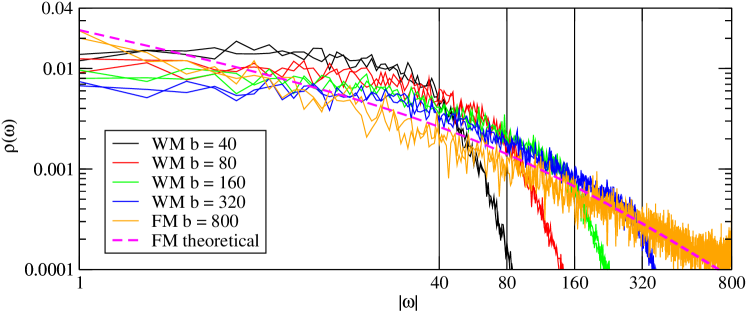
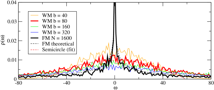
Figure 1: LDoS for the FM and for the WM via direct diagonalization of $1600\times 1600$ matrices with ${s=1.5}$ and ${\epsilon=1.44}$. Upper panel: The log-log scale emphasizes the universality of the tails up to $\omega_{c}$. Lower panel: The log-linear scale emphasizes the difference in the non-universal core component.

3 Time Scales

A dimensional analysis predicts the existence of 3 relevant time scales: The Heisenberg time $t_{\mbox{\tiny H}}$ which is related to the density of states $\varrho$; the semiclassical (correlation) time which is related to the bandwidth $\omega_{c}$; and the generalized Wigner times $t_{0}$ which is related to the perturbation strength:

$$t_{\mbox{\tiny H}} = 2\pi\varrho,\ \ \ \ \ \ t_{c}=2\pi/\omega_{c}$$ (3)

$$t_{0} = \left(\frac{2\pi\epsilon^{2}}{\bm{\Gamma}(3{-}s)\sin(s\pi/2)}\right)^{-{1}/{(2-s)}}\equiv\frac{1}{\gamma_{0}}$$ (4)

where $\bm{\Gamma}$ is the Gamma function. The numerical prefactor that we have incorporated into the definition in Eq.(4) will be explained later in Section.7. We shall refer to $\varrho^{-1}$ and to $\omega_{c}$ as the infrared and ultraviolate cutoffs of the theory. Our main interest is in the continuum limit. Assuming further that $\omega_{c}$ is irrelevant, one expects a decay that is determined by the generalized Wigner time $t_{0}$.

It should be clear that the existence of a cutoff free universal theory in the continuum limit for ${s\neq 1}$ is not self evident. In fact the natural expectation might be to have either infrared or ultraviolate cutoff dependence. Indeed we find that the 2nd moment of the spreading depends on the $\omega_{c}$ cutoff, while $t_{0}$ is reflected in the FM case but not in the WM case. But as far as $P(t)$ is concerned, we find that a one-parameter cutoff free universal theory exists.

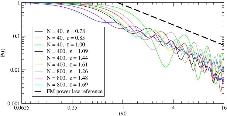
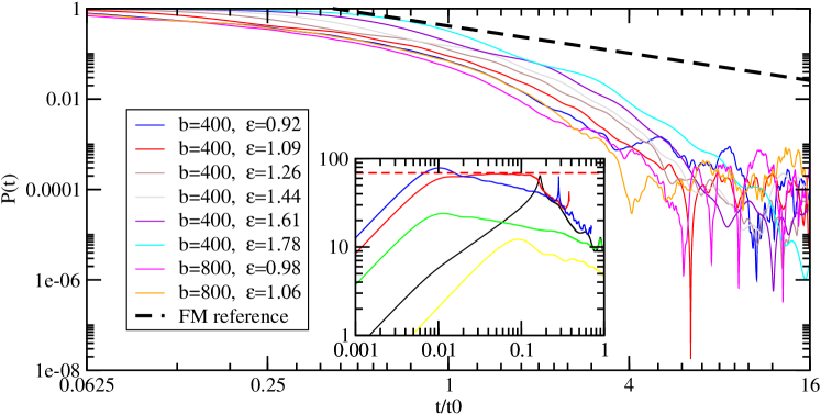
Figure 2: The survival probability $P(t)$ for the FM (top) and for the WM (bottom). The time is scaled with respect to $t_{0}$. For all curves in the main panels ${\varrho=1}$ and ${s=1.5}$. The WM simulations are presented in log-log scale in order to contrast it with the FM results. Inset: further analysis displaying $Y=-\ln[P(t)]/t$ vs $X=t$ in a log-log plot for representative runs with $(s,\epsilon)=$ black$(0.30,4.43)$, red$(1.00,3.24)$, green$(1.25,1.14)$, blue$(1.50,1.09)$, yellow$(1.75,0.50)$, showing that the decay in the WM case is described by a stretched exponential. The red bold dashed line has zero slope, corresponding to simple exponential decay for $s{=}1$.

4 The LDoS

Before analyzing the dynamics, it is important to understand the behavior of the Local Density of States (LDoS) [14], which is defined as follows:

$$\rho(\omega)=\sum_{\nu}|\langle\nu|0\rangle|^{2}\delta(\omega-(E_{\nu}{-}E_{0}))$$ (5)

where $|\nu\rangle$ are the eigenstates of the full Hamiltonian ${\cal H}$. An RMT averaging over realizations is implied in the WM case. Once the LDoS is computed, we can use it to calculate the survival probability:

$$P(t)\ \equiv\ \Big{|}\langle 0|\mbox{e}^{-i\mathcal{H}t}|0\rangle\Big{|}^{2}=\left|\mbox{FT}\Big{[}2\pi\rho(\omega)\Big{]}\right|^{2}$$ (6)

where FT denotes the Fourier transform. For flat bandprofile (${s=1}$), the LDoS $\rho(\omega)=(1/\gamma_{0})f(\omega/\gamma_{0})$ is a Lorentzian ${f(x)=(1/\pi)/(1+x^{2})}$ [14], leading to a Wigner exponential decay for $P(t)$. For (${s\neq 1}$) the ensuing analysis shows that $\rho(\omega)$ has a core-tail structure [16, 17, 12]. Namely, it consists of two distinct regions ${x\gg 1}$ and ${x<1}$ that reflect universal and non-universal features of the problem respectively. The tails ${x\gg 1}$ can be calculated using $1^{\mbox{\tiny st}}$ order perturbation theory leading to ${f(x)\propto 1/x^{3-s}}$. This component we regard as universal. The core (${x<1}$) reflects the non-perturbative mixing of the levels, and it is non-universal. In the WM case we argue that for ${x\ll 1}$ it is semicircle-like, while for FM we have a singular behaviour ${f(x)\sim x^{1-s}}$. These findings are supported by the numerical calculations of Fig.1, and are reflected in the behavior of $P(t)$ as confirmed by the numerical simulations of Fig.2.

5 Friedrichs model

Using the Schur complement technique, we can calculate analytically the LDoS for the FM. The Green function is $G_{00}(\omega)=\{[\omega{-}\Delta(\omega)]+i(\Gamma(\omega)/2)\}^{-1}$ with the standard notations $\Gamma(\omega)=\tilde{C}(\omega)$,

$$\Delta(\omega) = \mathchoice{{\vbox{\hbox{$\textstyle-$}}\kern-4.86108pt}}{{\vbox{\hbox{$\scriptstyle-$}}\kern-3.25pt}}{{\vbox{\hbox{$\scriptscriptstyle-$}}\kern-2.29166pt}}{{\vbox{\hbox{$\scriptscriptstyle-$}}\kern-1.875pt}}\!\int_{-\infty}^{+\infty}\frac{\widetilde{C}(\omega^{\prime})}{\omega-\omega^{\prime}}\ \frac{\mbox{d}\omega^{\prime}}{2\pi}$$ (7)

$$= \epsilon^{2}\pi\cot\left(s{\pi}/{2}\right)|\omega|^{s-1}\mbox{sgn}(\omega)$$

In the last line we performed the limit $\omega_{c}\rightarrow\infty$ (with the limiting expression converging in distribution). The LDoS of Eq.(5) is $-({1}/{\pi})\mbox{Im}\left[G_{00}(\omega)\right]$ leading to

$$\rho(\omega)=\frac{1}{\pi}\,\frac{\Gamma(\omega)/2}{(\omega-\Delta(\omega))^{2}+(\Gamma(\omega)/2)^{2}}$$ (8)

6 Wigner Model

The analysis of the LDOS for the WM can be carried out approximately using a combination of heuristic and formal methods. Our numerical results reported in Fig. 1 confirm that the LDoS has $1^{\mbox{\tiny st}}$ order tails ${|V_{n,0}/(E_{n}-E_{0})|^{2}}$ that co-exist with the core (non-perturbative) component. We can determine the border $\gamma_{0}$ between the core and the tail simply from the requirement ${p_{0}\sim 1}$ where

$$p_{0}=\int_{\gamma_{0}}^{\infty}\frac{\tilde{C}(\omega)}{\omega^{2}}\frac{d\omega}{2\pi}$$ (9)

For ${s>2}$ we would have for sufficiently small coupling ${p_{0}\ll 1}$ even if we took the limit $\gamma_{0}\rightarrow 0$. This means that $1^{\mbox{\tiny st}}$ order perturbation theory is valid as a global approximation. But for $s<2$ the above equation implies breakdown of $1^{\mbox{\tiny st}}$ order perturbation theory at $\gamma_{0}\sim\epsilon^{2/(2{-}s)}$. In the tails $\mathcal{H}_{0}$ dominates over $V$, while in the core $V$ dominates. Therefore, as far as the core in concerned, it makes sense to diagonalize $V$ with an effective cutoff $\gamma_{0}$. Following [18], the result for the LDoS lineshape should be semicircle-like, with width given by the expression

$$\Delta E_{\mbox{\tiny sc}}=\left[\int_{0}^{\gamma_{0}}\tilde{C}(\omega)\frac{d\omega}{2\pi}\right]^{1/2}$$ (10)

where above we use the effective bandwidth $\gamma_{0}$, which replaces the actual bandwidth $\omega_{c}$ (the latter would be appropriate as in [18] if we were considering the WM without the diagonal energies). The outcome of the integral is ${\Delta E_{\mbox{\tiny sc}}\sim\gamma_{0}}$, demonstrating that our procedure is self-consistent: the core has the same width as implied by the breakdown of $1^{\mbox{\tiny st}}$ order perturbation theory. We note that within this perspective the ${s=1}$ Lorentzian is regarded as composed of a semicircle-like core and $1^{\mbox{\tiny st}}$ order tails.

7 The survival probability

In the WM case the function $\rho(\omega)$ is smooth with power law tails ${\sim 1/\omega^{1+\alpha}}$ where ${\alpha=2{-}s}$. Thanks to the smoothness the FT does not have power law tails but is exponential-like. The similarity with the $\alpha$-stable Levy distribution suggests that $P(t)$ would be similar to a stretched exponential,

$$P(t)\approx \exp[-(t/t_{0})^{2{-}s}]$$ (11)

The expression for $t_{0}$ in Eq.(4) is implied by the observation that $1/|\omega|^{1{+}\alpha}$ tails are FT associated with a discontinuity $-C|t|^{\alpha}$, where ${C=[2\bm{\Gamma}(1{+}\alpha)\sin(\alpha\pi/2)]^{-1}}$.

In the FM case we observe that the function $\rho(\omega)$ in Eq.(8) features a crossover from ${\omega^{1{-}s}}$ for ${|\omega|\ll\gamma_{0}}$ to ${\Gamma(\omega)/\omega^{2}}$ for ${|\omega|\gg\gamma_{0}}$. Thus, compared with the WM case, the FT has an additional contribution from the singularity at $\omega{=}0$, and consequently by the Tauberian theorem [19], the survival amplitude has a non-exponential decay, that for sufficiently long time is described by a power law:

$$P(t)\ \ =\ \ \left|\frac{2\sin((s{-}1)\pi)}{(2{-}s)\pi\ (t/t_{0})^{2{-}s}}\right|^{2}$$ (12)

The long time behavior is dominated by the non-smooth feature of the core, and not by the tails. Comparing the exponential and the power-law we can find the expression for the crossover time $t_{0}^{\prime}$ that becomes ${t_{0}^{\prime}\sim[\log|s{-}1|]^{1/(2{-}s)}t_{0}\gg t_{0}}$ close to the Ohmic limit ($s{\sim}1$). For ${s=1}$ only the exponential decay survives. We emphasize that the cutoff independent behavior appears only after a short transient, i.e. for ${t>t_{c}}$. For completeness we note that for the FM with $s{=}2$ we get ${P(t)\approx|\log(t/t_{c}^{\prime})|^{2}}$, that holds for ${t_{c}<t<t_{c}^{\prime}}$ where ${t_{c}^{\prime}=t_{c}\mbox{e}^{1/(2\epsilon^{2})}}$. For ${s{>}2}$ there is an immediate but only partial decay that saturates at the value ${P(t)=|1{-}p_{0}|^{2}}$ for ${t>t_{c}}$.

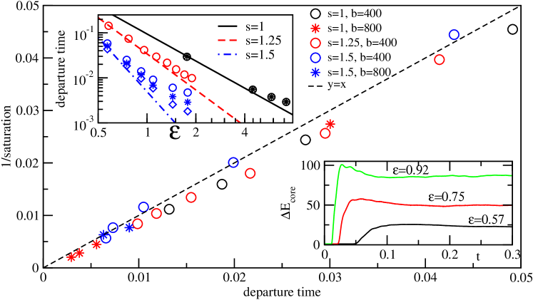
Figure 3: Lower Inset: Examples for the time evolution of $\Delta E_{\mbox{\tiny core}}$ for $s{=}1.5$ and $b{=}800$ in the WM case. Main panel: The extracted departure time versus the extracted inverse saturation value. This scatter diagram demonstrates the validity of one parameter scaling. Upper Inset: The extracted departure time versus the perturbation strength $\epsilon$. The theoretical (dashed) lines are based on the $t_{0}$ estimate of Eq.(4). The deviations of the departure time from the theoretical expectation diminish in the limit ${\omega_{c}\to\infty}$. The $\circ$ corresponds to $b=400$, the $\star$ to $b=800$, and the $\diamond$ to $b=1600$.

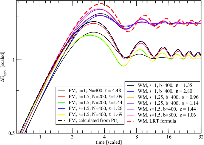
Figure 4: Scaled spread $\Delta E_{\mbox{\tiny sprd}}/(\omega_{c}^{s}\epsilon^{2}/s)^{1/2}$ versus scaled time ${\omega_{c}t}$ for the FM and the WM. The linear response theory (LRT) prediction Eq.(13), for the WM, as well as the exact result Eq.(14) for the FM are plotted for comparison.

8 Spreading

The distinction between core and tail components becomes physically transparent once we analyze the time dependent energy spreading of the wavepacket. Using the same time dependent analysis as in the ${s=1}$ case of Ref.[17], it is straightforward to show that the rise of $\Delta E_{\mbox{\tiny core}}(t)$ is at $t\sim t_{0}$, and its saturation value is ${\sim\gamma_{0}}$. Thus $\Delta E_{\mbox{\tiny core}}$ should exhibit one parameter scaling with respect to $t_{0}$. In Fig.3 we present the results of the numerical analysis. Our data, indicate that the expected one-parameter scaling is obeyed. We have verified that the slight deviation (shown in the inset) from the expected $\epsilon$ dependence is an artifact due to having finite (rather then infinite) bandwidth in the numerical simulation.

The physics of $\Delta E_{\mbox{\tiny sprd}}$ is quite different and not necessarily universal, because the second moment is dominated by the tails, and hence likely to depend on the cutoff $\omega_{c}$ and diverge in the limit $\omega_{c}\rightarrow\infty$. Indeed in the WM case we can use the Linear Response Theory (LRT) result of [17, 12]

$$\Delta E_{\mbox{\tiny sprd}}(t)=\left[2\Big{(}C(0)-C(t)\Big{)}\right]^{1/2}$$ (13)

where $C(t)$ is the inverse FT of $\tilde{C}(\omega)$. This gives the saturated value $(2\omega_{c}^{s}\epsilon^{2}/s)^{1/2}$ as soon as ${t>t_{c}}$. We now turn to the FM case. The solution of the Schrödinger equation for $c_{n}(t)$ is well known [2], and (setting $E_{0}{=}0$) can be expressed using the real amplitude $c(t){\equiv}c_{0}(t)$. In particular $P(t)=|c(t)|^{2}$ and also the energy spreading can be computed in a closed form, with the end result

$$\Delta E_{\mbox{\tiny sprd}}(t)=\Big{[}(1{+}c^{2}(t))C(0)-\dot{c}(t)^{2}+2c(t)\ddot{c}(t)\Big{]}^{1/2}\ \ \ \$$ (14)

For $t<t_{0}$ we can use the estimates ${c(t)\approx 1}$ and ${\dot{c}(t)\approx 0}$ and ${\ddot{c}(t)\approx-C(t)}$ to conclude that $\Delta E_{\mbox{\tiny sprd}}(t)$ behaves as in Eq.(13). But for ${t>t_{0}}$ we get

$$\Delta E_{\mbox{\tiny sprd}}(t)\approx\Big{[}(1{+}P(t))C(0)\Big{]}^{1/2}$$ (15)

leading to a saturation value smaller by factor $\sqrt{2}$, reflecting the non-stationary decay of the fluctuations as a function of time. More interestingly Eq.(14) contains a cutoff independent term that reflects the universal time scale $t_{0}$. The numerical results in Fig.4 confirm the validity of the above expressions. We note that in the FM case the effect of recurrences is more pronounced, because they are better synchronized: all the out-in-out traffic goes exclusively through the initial state.

9 Summary and Discussion

In this work we have compared two models that have the same spectral properties, but still different underlying dynamics. One of them has an integrable dynamics (FM) while the other is an RMT type (WM). This is complementary to our past work [20] where we have contrasted a physical model with its RMT counterpart.

Non-Ohmic coupling to the continuum emerges in various frameworks in physics. The general WM analysis might be motivated by the study of quantized chaotic systems that exhibit non-Ohmic fluctuations due to semi-classically implied long time power-law correlations. In fact typical power spectra are in general not like “white noise” (e.g. [16, 20, 12]). The general FM analysis might be motivated by studies of bound states that are embedded in the continuum as in the single-level Fano-Anderson model, with diverse realizations in the molecular / atomic / electronic context and also with implication regarding photonic lattices: see [21] and further references therein.

It should be clear that by considering two special models, we do not cover the full range of possibilities: In realistic circumstances the perturbation might have any rank, and there might be non-trivial correlations between off-diagonal elements (which was in fact the case in [20]). Still our results, since they relate to two extreme limiting models (FM,WM), serve to illuminate the limitations on the universality of Wigner’s theory.

In the non-Ohmic decay problem that we have considered a universal generalized Wigner time scale has emerged. It is not this time scale but rather the functional form of the decay that reflects the non-universality. We find that for “non-Ohmic chaos” (WM case) the survival probability becomes a stretched exponential beyond the Wigner time scale, which is both surprising and interesting. This is contrasted with the “integrable” power-law decay that takes over in the long time limit (FM case), and obviously very different from the Ohmic exponential result. Only the standard case of flat (Ohmic) bandprofile is fully universal.

It is worth mentioning that in a bosonic second quantized language the decay of the probability can be re-interpreted as the decay of the site occupation $\hat{n}$. If the interaction between the bosons is neglected this reduction is exact and merely requires an appropriate dictionary. In the latter context each level becomes a bosonic site which is formally like an harmonic oscillator, and hence the initially empty continuum is regarded as a zero temperature bath. Consequently the decay problem is formally re-interpreted as a quantum dissipation problem with an Ohmic ($s{=}1$) or non-Ohmic ($s{\neq}1$) bath. The time scale $t_{0}$ is associated with the damped motion of the generalized coordinate $\hat{n}$. Optionally $P(t)$ could be related to dephasing, and in this case $t_{0}$ is reinterpreted as the coherence time, as in Landau’s Fermi liquid theory.

References

Note after publication:– This 2009 arXiv submission has been published in J. Phys. A 43, 095301 (2010). A follow up that contains some more recent additional results, and full derivations that were not included in this short report is available [arXiv:1003.1645], and has been published in Phys. Rev. E 81, 036219 (2010). There is another follow up regarding “Quantum anomalies and linear response theory” [arXiv:1003.3303].

References

- [1] N. Auerbach, V. Zelevinsky, Phys. Rev. C 65, 034601 (2002); V.V. Sokolov, V.G. Zelevinsky, Nucl. Phys. A 504, 562 (1989).
- [2] C. Cohen-Tannoudji, J. Dupont-Roc, G. Grynberg, Atoms-Photon Interactions: Basic Processes and Applications (Wiley, New-York, 1992).
- [3] M.A. Nielsen and I.L. Chuang, Quantum computation and quantum information (Cambridge University Press,2000).
- [4] V.N. Prigodin, B.L. Altshuler, K.B. Efetov, S. Iida, Phys. Rev. Lett. 72, 546 (1994); B.L. Altshuler et al., Phys. Rev. Lett. 78, 2803 (1997).
- [5] C. W. J. Beenakker, H. van Houton, in Solid State Physics: Advances in Research and Applications, Ed. H. Ehrenreich and D. Turnbull, 1-228 44 (Academic Press, New York, 1991).
- [6] E. Persson, I. Rotter, H.-J. Stöckmann, M. Barth, Phys. Rev. Lett. 85, 2478 (2000).
- [7] V. Weisskopf and E.P. Wigner, Z. Phys. 63, 54 (1930).
- [8] F.M. Izrailev, A.Castaneda-Mendoza, Phys. Lett. A 350, 355 (2006); V.V. Flambaum, F.M.Izrailev, Phys. Rev. E 64 026124 (2001); V.V. Flambaum, F.M.Izrailev, Phys. Rev.E 61, 2539 (2000).
- [9] Y.V. Fyodorov, O.A. Chubykalo, F.M. Izrailev, G. Casati, Phys. Rev. Lett. 76, 1603 (1996).
- [10] J.L. Gruver et al., Phys. Rev E 55, 6370 (1997).
- [11] P.G. Silvestrov, Phys. Rev. B 64, 113309 (2001); A. Amir, Y. Oreg, Y. Imry, Phys. Rev. A 77, 050101(R) (2008).
- [12] M. Hiller, D. Cohen, T. Geisel and T. Kottos, Annals of Physics 321, 1025 (2006).
- [13] K.O. Friedrichs, Comm. Pure Appl. Math. 1, 361 (1948).
- [14] E. Wigner, Ann. Math 62 548 (1955); 65 203 (1957).
- [15] A. Barnett, D. Cohen and E.J. Heller, Phys. Rev. Lett. 85, 1412 (2000); J. Phys. A 34, 413-437 (2001).
- [16] D. Cohen, E.J. Heller, Phys. Rev. Lett. 84, 2841 (2000).
- [17] D. Cohen, F.M. Izrailev, T. Kottos, Phys. Rev. Lett. 84, 2052 (2000). T. Kottos and D. Cohen, Europhys. Lett. 61, 431 (2003).
- [18] M. Feingold, Europhysics Letters 17, 97 (1992).
- [19] K. Soni, R.P. Soni, J. Math. Anal. Appl. 49, 477 (1975).
- [20] D. Cohen and T. Kottos, Phys. Rev. E 63, 36203 (2001).
- [21] S. Longhi, Phys. Rev. Lett. 97, 110402 (2006); Eur. Phys. J. B 57, 45 (2007).