Resolving mixing in Smoothed Particle Hydrodynamics

Abstract

Standard formulations of smoothed particle hydrodynamics (SPH) are unable to resolve mixing at fluid boundaries. We use an error and stability analysis of the generalised SPH equations of motion to prove that this is due to two distinct problems. The first is a leading order error in the momentum equation. This should decrease with increasing neighbour number, but does not because numerical instabilities cause the kernel to be irregularly sampled. We identify two important instabilities: the clumping instability and the banding instability, and we show that both are cured by a suitable choice of kernel. The second problem is the local mixing instability (LMI). This occurs as particles attempt to mix on the kernel scale, but are unable to due to entropy conservation. The result is a pressure discontinuity at boundaries that pushes fluids of different entropy apart. We cure the LMI by using a weighted density estimate that ensures that pressures are single valued throughout the flow. This also gives a better volume estimate for the particles, reducing errors in the continuity and momentum equations. We demonstrate mixing in our new Optimised Smoothed Particle Hydrodynamics (OSPH) scheme using a Kelvin Helmholtz instability (KHI) test with density contrast 1:2, and the ‘blob test’ – a 1:10 density ratio gas sphere in a wind tunnel – finding excellent agreement between OSPH and Eulerian codes.

1 Introduction

Smoothed Particle Hydrodynamics (SPH) was first introduced as a tool for studying stellar structure (Gingold & Monaghan 1977; Lucy 1977), but has since found wide application in all areas of theoretical astrophysics (Monaghan, 1992), in engineering (Libersky et al., 1993), and beyond (e.g. Hieber & Koumoutsakos 2008).

Although there are many varieties of SPH, the central idea is to represent a fluid by discrete particles that move with the flow (Monaghan 1992; Price 2005). Typically these particles represent the fluid exactly, though in some variants the fluid is advected on top of the particles (Dilts 1999; Maron & Howes 2003). The key advantages over Eulerian schemes are its Lagrangian nature that makes it Galilean invariant, and its particle nature that makes it easy to couple to the fast multipole method for gravity that scales as $O(N)$ (Dehnen 2000; Greengard & Rokhlin 1987). However, SPH has problems correctly integrating fluid instabilities and mixing at boundaries (Morris 1996b; Dilts 1999; Ritchie & Thomas 2001; Marri & White 2003; Agertz et al. 2007). Several different reasons have been suggested for this in the literature so far. Morris (1996b) and Dilts (1999) argue that the problem owes to errors in the SPH gradients that do not show good convergence for irregular particle distributions. Price (2007) argue that the problem owes to the fact that entropies are discontinuous at boundaries, while the densities are smooth. This gives spurious pressure blips at boundaries that drive fluids of different entropy apart. They find that adding thermal conductivity at boundaries to smooth the entropies gives improved mixing in SPH. Wadsley et al. (2008) make a similar argument, phrasing the problem in terms of an inability for SPH particles to mix and generate entropy on the kernel scale. They find that adding a heat diffusion term to model subgrid turbulence gives improved mixing in SPH. Finally, Ritchie & Thomas (2001) suggest that the problem lies in the SPH density estimate. They introduce a new temperature weighted density estimate that is designed to give smoother pressures at flow boundaries, thus combating the spurious boundary pressure blip.

In this paper, we perform an error and stability analysis of SPH in its most general form to understand why mixing fails. In doing this, we show that all of the above authors correctly identified one of two distinct problems with mixing in SPH. The first is an $O(h^{-1})$ error in the momentum equation identified by Morris (1996b) and Dilts (1999). The second relates to entropy conservation on the kernel scale, as addressed directly by Price (2007) and Wadsley et al. (2008), and indirectly by Ritchie & Thomas (2001). Having identified the problem, we present a new method – Optimised Smoothed Particle Hydrodynamics (OSPH) – that, given sufficient resolution, correctly resolves multiphase fluid flow.

This paper is organised as follows. In §2 and §3, we briefly review standard SPH schemes and introduce our new OSPH scheme. We show that there are two distinct problems with mixing in SPH: the ‘${\bf E}_{0}$ error’ in the momentum equation, and the ‘local mixing instability’ (LMI), and we show how both can be cured. In §4, we present our implementation of OSPH in the GASOLINE code (Wadsley et al., 2004). In §5, we use a Kelvin Helmholtz instability (KHI) test with density contrast 1:2 and 1:8 to demonstrate mixing in OSPH. We show the effect of turning on each of the OSPH improvements one at a time, arriving at a solution that is in excellent agreement with the Eulerian code RAMSES (Teyssier, 2002). In §6, we use the standard Sod shock tube test to demonstrate that OSPH can successfully model shocks. In §7, we revisit the ‘blob test’ introduced in Agertz et al. (2007), finding excellent agreement between OSPH and the Eulerian code FLASH (Fryxell et al., 2000). Finally, in §8 we present our conclusions.

2 Smoothed Particle Hydrodynamics

In SPH, the fluid is represented by discrete particles that move with the flow. The density of each particle is estimated by a weighted sum over its neighbours:

$$\rho_{i}=\sum_{j}^{N}m_{j}W(|{\bf r}_{ij}|,h_{i})$$ (1)

where $h_{i}$ and $m_{j}$ are the smoothing length and mass of particle $i$ and $j$, respectively; we define ${\bf r}_{ij}={\bf r}_{i}-{\bf r}_{j}$ and similarly for other vectors; and $W$ is a symmetric kernel that obeys the normalisation condition:

$$\int_{V}W(|{\bf r}-{\bf r}^{\prime}|,h)\mathrm{d}^{3}{r}^{\prime}=1$$ (2)

and the property:

$$\lim_{h\rightarrow 0}W(|{\bf r}-{\bf r}^{\prime}|,h)=\delta(|{\bf r}-{\bf r}^{\prime}|)$$ (3)

In the limit $N\rightarrow\infty,h\rightarrow 0$ (and using $m_{j}/\rho_{j}\rightarrow\mathrm{d}^{3}{r}^{\prime}$) equation 1 recovers the continuum flow density.

The equations of motion for SPH are then derived by discretising the Euler equations – the continuity, momentum and energy equations:

$$\frac{d\rho}{dt}=-\rho{\bf\nabla}\cdot{\bf v}$$ (4)

$$\frac{d{\bf v}}{dt}=-\frac{{\bf\nabla}P}{\rho}$$ (5)

$$\frac{du}{dt}=-\frac{P}{\rho}{\bf\nabla}\cdot{\bf v}$$ (6)

where $\rho,v$ and $u$ are the density, velocity and internal energy per unit mass of the flow, respectively.

The Euler equations can be derived from the Lagrangian for hydrodynamics (e.g. Bennett 2006):

$$L=\int\left(\frac{1}{2}\rho v^{2}-\rho u\right)dV$$ (7)

and in many modern derivations of the equations of motion for SPH, equation 7 is discretised, rather than equations 4-6.

Replacing the volume element $dV$ with the volume per SPH particle $m/\rho$, we obtain (Price 2005):

$$L=\sum_{j}m_{j}\left(\frac{1}{2}{\bf v}_{j}^{2}-u_{j}\right)$$ (8)

and the standard SPH equations of motion then follow from the Euler-Lagrange equations:

$$\frac{d\rho_{i}}{dt}=\sum_{j}^{N}m_{j}{\bf v}_{ij}\cdot{\bf\nabla}_{i}W_{ij}$$ (9)

$$\frac{d{\bf v}_{i}}{dt}=-\sum_{j}^{N}m_{j}\left[\frac{P_{i}}{\rho_{i}^{2}}+\frac{P_{j}}{\rho_{j}^{2}}\right]{\bf\nabla}_{i}W_{ij}$$ (10)

$$\frac{du_{i}}{dt}=\frac{P_{i}}{\rho_{i}^{2}}\sum_{j}^{N}m_{j}{\bf v}_{ij}\cdot{\bf\nabla}_{i}W_{ij}$$ (11)

where $W_{ij}=W(|{\bf r}_{ij}|,h_{i})$.

Note that equation 9 is automatically satisfied by time derivative of the SPH density estimate (equation 1). For this reason, equation 1 is often referred to as the integral form of the continuity equation.

The above system of equations are closed by the equation of state:

$$P_{i}=u_{i}\left(\gamma-1\right)\rho_{i}$$ (12)

This standard approach to deriving the SPH equations of motion has the advantage that the resulting equations are coherent by construction – that is they are consistent with a Lagrangian. This gives very good conservation properties for the flow. It is also straightforward to calculate the necessary correction terms that arise if the smoothing lengths are a function of space and time $h=h({\bf r},t)$ (see e.g. Nelson & Papaloizou 1994; Price 2005). We do not include these correction terms in this paper.

However, this standard derivation leads to a scheme that cannot correctly model fluid mixing processes (see §1), which motivates us to move to a more general derivation. Discretising each of the Euler equations separately leads to a free function for each equation: $\eta$, $\phi$ and $\zeta$, as well as a different smoothing kernel for each. This is the approach we take next in §3. In §3.3 and §3.4, we will then use an error and stability analysis of these more general equations of motion to constrain the new functions $\eta,\phi$ and $\zeta$ and our new kernels. By choosing these new free functions and kernels such that they minimise the integration error, we will arrive at a new scheme that can, with sufficient resolution, correctly resolve multiphase fluid flow.

3 OPTIMISED Smoothed Particle Hydrodynamics

In the previous section, we presented a standard derivation of the SPH equations of motion. However, this standard derivation leads to a scheme that cannot correctly model fluid mixing processes (see §1). In this section, we move to a more general derivation of the SPH equations of motion. We show that, in general, we have a free function for each of the Euler equations: $\eta$, $\phi$ and $\zeta$, as well as a different smoothing kernel for each. There is also a freedom in the energy equation in the choice of integration variable (energy or entropy; §3.2). In §3.3 and §3.4, we will then use an error and stability analysis of these more general equations of motion to constrain the new functions $\eta,\phi$ and $\zeta$ and our new kernels. By choosing these new free functions and kernels such that they minimise the integration error, we will arrive at a new scheme that can, with sufficient resolution, correctly resolve multiphase fluid flow.

3.1 A general derivation of SPH

In general, we have some freedom in how we discretise the Euler equations (equations 4-6) to obtain the equations of motion for SPH (see e.g. Monaghan, 1992; Price, 2005; Rosswog, 2009). The gradients in the Euler equations can be expanded to include a new free function for each equation: $\eta$, $\phi$ and $\zeta$:

$$\frac{d\rho}{dt}=\eta\left[{\bf v}\cdot{\bf\nabla}\left(\frac{\rho}{\eta}\right)-{\bf\nabla}\cdot\left(\frac{\rho{\bf v}}{\eta}\right)\right]$$ (13)

$$\frac{d{\bf v}}{dt}=-\left[\frac{P\phi}{\rho^{2}}{\bf\nabla}\left(\frac{\rho}{\phi}\right)+\frac{1}{\phi}{\bf\nabla}\left(\frac{P\phi}{\rho}\right)\right]$$ (14)

$$\frac{du}{dt}=\frac{P}{\rho^{2}}\zeta\left[{\bf v}\cdot{\bf\nabla}\left(\frac{\rho}{\zeta}\right)-{\bf\nabla}\cdot\left(\frac{\rho{\bf v}}{\zeta}\right)\right]$$ (15)

In the continuum form, above, $\eta,\phi$ and $\zeta$ cancel. But in the discrete SPH form, they remain giving a useful additional freedom (Price, 2005):

$$\frac{d\rho_{i}}{dt}=\sum_{j}^{N}m_{j}\frac{\eta_{i}}{\eta_{j}}{\bf v}_{ij}\cdot\overline{H}_{ij}{\bf r}_{ij}$$ (16)

$$\frac{d{\bf v}_{i}}{dt}=-\sum_{j}^{N}m_{j}\left[\frac{P_{i}}{\rho_{i}^{2}}\frac{\phi_{i}}{\phi_{j}}+\frac{P_{j}}{\rho_{j}^{2}}\frac{\phi_{j}}{\phi_{i}}\right]\overline{K}_{ij}{\bf r}_{ij}$$ (17)

$$\frac{du_{i}}{dt}=\frac{P_{i}}{\rho_{i}^{2}}\sum_{j}^{N}m_{j}\frac{\zeta_{i}}{\zeta_{j}}{\bf v}_{ij}\cdot\overline{L}_{ij}{\bf r}_{ij}$$ (18)

where $\overline{H}_{ij}=\left[H(|{\bf r}_{ij}|,h_{i})+H(|{\bf r}_{ij}|,h_{j})\right]/2$, $\overline{K}_{ij}$ and $\overline{L}_{ij}$ are symmetrised smoothing kernels – one for each Euler equation. Standard SPH (SPH from here on) is a special case of the above with $\eta=\phi=\zeta=1$ and $\overline{H}_{ij}{\bf r}_{ij}=\overline{K}_{ij}{\bf r}_{ij}=\overline{L}_{ij}{\bf r}_{ij}={\bf\nabla}_{i}\overline{W}_{ij}$.

Equation 16 casts the continuity equation in differential form. This is problematic since, in this case, the particles no longer represent the fluid exactly. Instead they represent a moving mesh on which the Euler equations are solved. This leads to the danger that high density regions will contain few particles leading to large errors (Maron & Howes, 2003). For this reason, we use instead a generalised integral form for the continuity equation:

$$\rho_{i}=\sum_{j}^{N}m_{j}\frac{\eta_{i}}{\eta_{j}}\overline{W}_{ij}$$ (19)

which, taking the time derivative, gives:

$$\frac{d\rho_{i}}{dt}=\sum_{j}^{N}m_{j}\frac{\eta_{i}}{\eta_{j}}{\bf v}_{ij}\cdot{\bf\nabla}_{i}\overline{W}_{ij}+\epsilon$$ (20)

where:

$$\epsilon=\sum_{j}^{N}m_{j}\left(\frac{\dot{\eta}_{i}}{\eta_{i}}-\frac{\dot{\eta}_{j}}{\eta_{j}}\right)\frac{\eta_{i}}{\eta_{j}}\overline{W}_{ij}$$ (21)

and $\dot{\eta}=\frac{d\eta}{dt}$.

This reduces to the continuity equation (equation 16) under the kernel constraint: $\overline{H}_{ij}{\bf r}_{ij}={\bf\nabla}_{i}\overline{W}_{ij}$, and for $\epsilon=0$. The latter can be satisfied by construction if $\eta_{i}=\eta_{j}$ (as is the case for SPH), or if $\dot{\eta}=0$. However, in the continuum limit ($N\rightarrow\infty$, $h\rightarrow 0$), $\epsilon\rightarrow 0$ and so $\epsilon$ will vanish with increasing resolution. For this reason, equation 19 gives a valid approximation to the continuity equation for any choice of $\eta$, with $\epsilon$ simply contributing an additional error term.

3.2 Energy versus entropy forms of SPH

A final freedom in the equations motion for SPH comes from the energy equation. Equation 18 is the standard energy form of SPH, but there is also an entropy form (Goodman & Hernquist 1991; Springel & Hernquist 2002). Instead of the internal energy, $u$, we evolve a function $A(s)$ – the entropy function – that is a monotonic function of the entropy $s$ defined by the equation of state:

$$P_{i}=A_{i}(s)\rho_{i}^{\gamma}$$ (22)

Away from shocks and in the absence of thermal sources or sinks, $A_{i}$ is a constant of motion. Thus, taking the time derivative of equation 22 and substituting for equation 12, we recover:

$$\frac{du_{i}}{dt}=\frac{P_{i}}{\rho_{i}^{2}}\frac{d\rho_{i}}{dt}$$ (23)

by construction. Schemes that obey equation 23 are called thermodynamically consistent.

In practice, we find – for the tests presented in this paper – that the energy and entropy forms of SPH give near-identical results, provided that equation 23 is satisfied (for adiabatic flow). We use the thermodynamically consistent energy form throughout this paper. This gives us the constraints: $\zeta=\eta$ and $\overline{L}_{ij}{\bf r}_{ij}=\overline{H}_{ij}{\bf r}_{ij}={\bf\nabla}_{i}\overline{W}_{ij}$, which we apply from here on. We also use $\overline{K}_{ij}{\bf r}_{ij}={\bf\nabla}_{i}\overline{W}_{ij}$, as in standard SPH. This is not a formal requirement, but ensures that coherence is recovered in the limit of constant density.

3.3 Errors: choosing the free functions

In this section, we perform an error analysis of the generalised equations for SPH (equations 17, 18 and 19) derived in §3.1. We will then choose our free functions $\eta$, $\phi$ and $\zeta$ so that these errors are minimised.

3.3.1 Error analysis

We assume that the pressure and velocity of the flow are smooth. In this case, we can Taylor expand to give:

$$P_{j}\simeq P_{i}+h{\bf x}_{ij}\cdot{\bf\nabla}_{i}P_{i}+O(h^{2})$$ (24)

and

$${\bf v}_{j}\simeq{\bf v}_{i}+h({\bf x}_{ij}\cdot{\bf\nabla}_{i}){\bf v}_{i}+O(h^{2})$$ (25)

where ${\bf x}_{ij}={\bf r}_{ij}/h$, and we have assumed a constant smoothing length $h$.

Substituting equations 24 and 25 into the continuity and momentum equations gives:

$$\frac{d\rho_{i}}{dt}\simeq-\rho_{i}\left({\bf R}_{i}{\bf\nabla}_{i}\right)\cdot{\bf v}_{i}+\epsilon+O(h)$$ (26)

and

$$\frac{d{\bf v}_{i}}{dt}\simeq-\frac{P_{i}}{h\rho_{i}}{\bf E}_{0,i}-\frac{\left({\bf V}_{i}{\bf\nabla}_{i}\right)P_{i}}{\rho_{i}}+O(h)$$ (27)

where ${\bf E}_{0,i}$ is a dimensionless error vector given by:

$${\bf E}_{0,i}=\sum_{j}^{N}\frac{m_{j}}{\rho_{j}}\left[g_{ij}+g^{-1}_{ij}\right]{\bf\nabla}^{x}_{i}\overline{W}_{ij}$$ (28)

and ${\bf R}_{i}$ and ${\bf V}_{i}$ are dimensionless error matrices given by:

$${\bf R}_{i}=\sum_{j}^{N}\frac{m_{j}}{\rho_{j}}f_{ij}{\bf S}_{ij}\qquad;\qquad{\bf V}_{i}=\sum_{j}^{N}\frac{m_{j}}{\rho_{j}}g^{-1}_{ij}{\bf S}_{ij}$$ (29)

with:

$${\bf S}_{ij}=\frac{1}{x}\frac{\partial\overline{W}_{ij}}{\partial x}\left(\begin{array}[]{ccc}x_{ij}^{2}&x_{ij}y_{ij}&x_{ij}z_{ij}\\ y_{ij}x_{ij}&y_{ij}^{2}&y_{ij}z_{ij}\\ z_{ij}x_{ij}&z_{ij}y_{ij}&z_{ij}^{2}\end{array}\right)$$ (30)

where ${\bf\nabla}^{x}_{i}=h{\bf\nabla}_{i}$; ${\bf x}_{ij}=(x_{ij},y_{ij},z_{ij})$; $x=|{\bf x}_{ij}|$; $f_{ij}=\frac{\rho_{j}}{\rho_{i}}\frac{\eta_{i}}{\eta_{j}}$; and $g_{ij}=\frac{\rho_{j}}{\rho_{i}}\frac{\phi_{i}}{\phi_{j}}$.

The accuracy of the continuity equation (26) is given by the extent to which $\epsilon=0$ (see equation 21) and ${\bf R}_{i}={\bf I}$, the identity matrix. The accuracy of the momentum equation (27) is given by the extent to which ${\bf E}_{0,i}={\bf 0}$ and ${\bf V}_{i}={\bf I}$. (The energy equation behaves similarly to the continuity equation with $\epsilon=0$.)

3.3.2 Minimising errors: the continuity equation

Let us consider how accurately equation 26 approximates its Euler equation equivalent (equation 4). First, consider standard SPH where $\eta=1$ and $\epsilon=0$ by construction. Typically in the literature, the error is calculated only in the continuum limit ($N\rightarrow\infty$; $h\rightarrow 0$; see e.g. Price (2005)). In this case, the sums become integrals, and (using $m_{j}/\rho_{j}\rightarrow\mathrm{d}^{3}{x}^{\prime}$) we obtain terms like:

$$\lim_{N\rightarrow\infty}{\bf R}_{33}({\bf x})=\int_{V}\mathrm{d}^{3}{x}^{\prime}f({\bf x},{\bf x}^{\prime})\frac{(z-z^{\prime})^{2}}{|{\bf x}-{\bf x}^{\prime}|}\frac{\partial W}{\partial x}$$ (31)

and

$$\lim_{N\rightarrow\infty}{\bf R}_{12}({\bf x})=\int_{V}\mathrm{d}^{3}{x}^{\prime}f({\bf x},{\bf x}^{\prime})\frac{(x-x^{\prime})(y-y^{\prime})}{|{\bf x}-{\bf x}^{\prime}|}\frac{\partial W}{\partial x}$$ (32)

where the notation ₃₃ refers to element $[3,3]$ in the matrix ${\bf R}$.

If we assume smooth densities, then we can Taylor expand $f$ also to obtain:

$$f=\frac{\rho({\bf r}^{\prime})}{\rho({\bf r})}\simeq 1+h\frac{({\bf x}-{\bf x}^{\prime})}{\rho}\cdot{\bf\nabla}\rho+O(h^{2})$$ (33)

and we see that, by symmetry of $W$, ${\bf R}={\bf I}$ to $O(h^{2})$. In fact, Taylor expanding to an order higher than above, it is straightforward to show that the whole continuity equation is accurate to $O(h^{2})$ in the limit $N\rightarrow\infty$ (see e.g. Price 2005). A similar argument applies to the other SPH equations of motion and leads to the conclusion that SPH is accurate to $O(h^{2})$. However – and this is a key point – this formal calculation is only valid for smoothly distributed particles in the limit $N\rightarrow\infty$. In practical situations, where we have a finite number of particles within the kernel and these are not perfectly smoothly distributed, the leading order errors in the continuity equation appear at $O(0)$ and are contained within the matrix ${\bf R}$. We will quote orders of error from here on in this finite particle limit.

We can think of each term of ${\bf R}$ as a finite sum approximation to a dimensionless integral that should be either 0 (for the off diagonal terms), or 1 (for the diagonal terms). For smooth particle distributions, this approximation is a good one since $f_{ij}\simeq 1$, while $m_{j}/\rho_{j}$ gives a good estimate of the volume of each particle within the kernel. However, if the particles are distributed irregularly on the kernel scale – for example at a sharp density step – then $f_{ij}$ can grow arbitrarily large, while $m_{j}/\rho_{j}$ becomes a poor volume estimate. We will demonstrate this in §5.

We can improve matters by choosing $\eta=\rho$, which fixes $f=1$ always. However, the integral form of the continuity equation then becomes:

$$\rho_{i}=\sum_{j}^{N}\frac{\rho_{i}}{\rho_{j}}m_{j}\overline{W}_{ij}$$ (34)

which must be solved iteratively and is not guaranteed to converge. Worse still, $\epsilon$ is now no longer zero and contributes an additional error.

Ritchie & Thomas (2001) present an interesting solution to this dilemma. If the pressures are approximately constant across the kernel ($P_{i}\simeq P_{j}$) then, for the energy form of SPH (see equation 12 and §3.2), $\frac{\rho_{i}}{\rho_{j}}\simeq\frac{u_{j}}{u_{i}}$ and equation 34 is well approximated by the integral continuity equation:

$$\rho_{i}=\sum_{j}^{N}\frac{u_{j}}{u_{i}}m_{j}\overline{W}_{ij}$$ (35)

This can be solved without the need for iteration.

The above suggests that we use $\eta=1/u$. Thermodynamic consistency then requires that we set $\zeta=\eta=1/u$ (see §3.2).

There may be some advantage, however, to using the entropy form of SPH. In this case, the equation of state is given by equation 22. For approximately constant pressure across the kernel, we now have that $\frac{\rho_{i}}{\rho_{j}}=\left(\frac{A_{j}}{A_{i}}\right)^{\frac{1}{\gamma}}$, and the integral continuity equation becomes:

$$\rho_{i}=\sum_{j}^{N}\left(\frac{A_{j}}{A_{i}}\right)^{\frac{1}{\gamma}}m_{j}\overline{W}_{ij}$$ (36)

This has the advantage that, in the absence of shocks or thermal sources/sinks, $\dot{A}=0$ and so the error term $\epsilon=0$ by construction (see equation 21). In practice, however, we find no appreciable difference between the energy and entropy forms of SPH for the tests presented in this paper. This suggests that $\epsilon$ is not a significant source of error.

Equations 35 and 36 retain the desirable integral form for the density, while giving significantly improved error properties. They also have a second important advantage that we discuss in §3.5. We refer to equation 35 as the ‘RT’ density estimator for the energy form of SPH; and equation 36 as the RT density estimator in the entropy form.

Cubic Spline (CS) kernel:

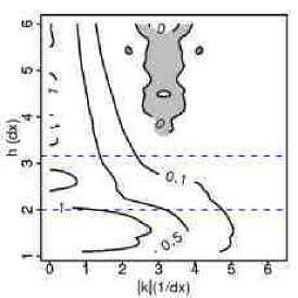
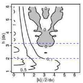
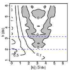
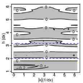
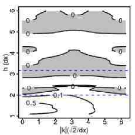
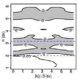
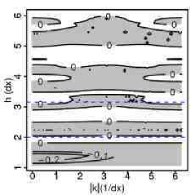
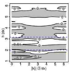
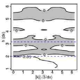
Figure 1: Stability plots for the Cubic Spline (CS) kernel (equation 44) in OSPH. The plots show contours of the frequency $\omega^{2}/k^{2}/c_{s}^{2}$ of plane waves impacting a regular lattice of particles, as a function of the wavenumber $k$ and the smoothing length $h$, in units of the inter-particle spacing $dx=1$. From left to right the plots show $(k_{x},k_{y},k_{z})=k(1,0,0),k(1,1,0)$ and $k(1,1,1)$. The three rows show the longitudinal wave and the two transverse waves for each of these orientations. Also marked by the blue dashed lines are the $h$ that corresponds to 32 neighbours (bottom line) and 128 neighbours (top line). OSPH is unstable if $\omega^{2}<0$ (grey regions).

Core Triangle (CT) kernel:

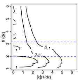
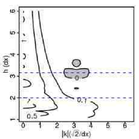
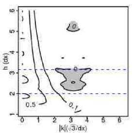
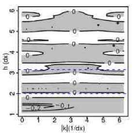
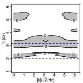
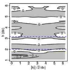
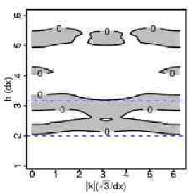
Figure 2: As Figure 1, but for the Core Triangle (CT) kernel.

High Order Core Triangle HOCT4 kernel:

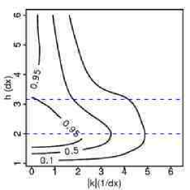
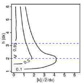
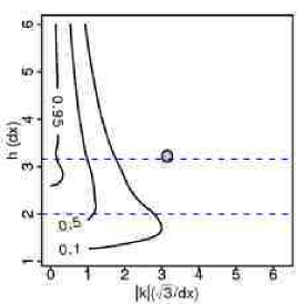
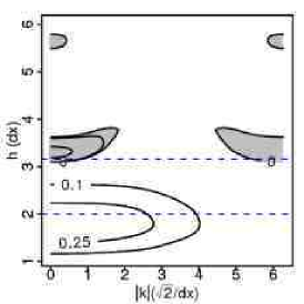
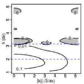
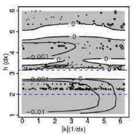
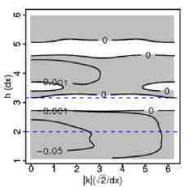
Figure 3: As Figure 1, but for the High Order Core Triangle (HOCT) kernel with $n_{k}=4$.

3.3.3 Minimising errors: the momentum equation

The momentum equation (equation 27) is more problematic than the continuity equation. Its accuracy is governed not only by the extent to which ${\bf V}_{i}={\bf I}$, but primarily by the leading ${\bf E}_{0,i}$ term that should vanish.

First, consider the situation in standard SPH where $\phi=1$ and $g_{ij}=\rho_{j}/\rho_{i}$. As for the continuity equation, in the continuum limit ($N\rightarrow\infty;h\rightarrow 0$), ${\bf E}_{0}={\bf 0}+O(h^{2})$ since ${\bf\nabla}^{x}_{i}\overline{W}_{ij}$ is antisymmetric. However, this analysis is only relevant if the particles are smoothly distributed on the kernel scale. For irregularly distributed particles, $g_{ij}$ can grow arbitrarily large, while $m_{j}/\rho_{j}$ is not guaranteed to be a good volume estimate. In such situations, ${\bf E}_{0}$ contributes a significant error. Worse still, moving to higher resolution is not guaranteed to help. In order for the SPH integration to converge as $h\rightarrow 0$, we require that ${\bf E}_{0,i}$ shrinks faster than $\frac{P_{i}}{h\rho_{i}}$. This requires some care in making sure that $h$ does not shrink too fast as the number of particles is increased.

A density step is an extreme example of an irregular particle distribution, and this suggests that the ${\bf E}_{0}$ error is at least in part responsible for SPH’s failure to correctly model mixing processes between different fluid phases. We demonstrate this in §5.

There are three key problems with ensuring that $\frac{P_{i}}{h\rho_{i}}{\bf E}_{0,i}$ will shrink with increasing resolution. The first is the function $g_{ij}$. In SPH, this is the ratio $\rho_{j}/\rho_{i}$ which is large when there are large density gradients. We can significantly improve on this we choose our free function $\phi=\rho$. In this case, we have $g_{ij}=g_{ij}^{-1}=1$ by construction, and $g_{ij}$ no longer contributes to the ${\bf E}_{0}$ error even for large density gradients across the kernel. The second problem relates to kernel scale smoothness. If particles clump or band on the kernel scale, then we will have poor kernel sampling and ${\bf E}_{0}$ will not approach its integral limit even at very high resolution. Ensuring that this does not happen means ensuring that our OSPH scheme is stable to perturbations. We discuss this next in §3.4. The third and final problem is the volume estimate of each particle $m_{j}/\rho_{j}$. This will be poor if the particles are irregularly distributed on the kernel scale (for example at a density step) leading to a large ${\bf E}_{0}$ error. We discuss this further in §3.5.

The choices $\zeta=\eta=1/u$; $\phi=\rho$ and the kernel constraints $\overline{H}_{ij}{\bf r}_{ij}=\overline{L}_{ij}{\bf r}_{ij}=\overline{K}_{ij}{\bf r}_{ij}={\bf\nabla}_{i}\overline{W}_{ij}$ are the first important ingredients in our OSPH scheme. These choices mean that we are no longer coherent, but this only introduces tolerable $O(h^{2})$ errors in the energy conservation (Hernquist & Katz, 1989).

3.4 Stability: the choice of kernel function

In §3.3, we used an error analysis of the generalised SPH equations of motion to show that the dominant source of error in SPH is in the momentum equation – the ${\bf E}_{0}$ error. We showed that choosing the free functions $\zeta=\eta=1/u$; $\phi=\rho$ and the kernel constraints $\overline{H}_{ij}{\bf r}_{ij}=\overline{L}_{ij}{\bf r}_{ij}=\overline{K}_{ij}{\bf r}_{ij}={\bf\nabla}_{i}\overline{W}_{ij}$ should minimise both this error and errors in the continuity equation, and we called these choices OSPH.

In OSPH, provided the particles are regularly distributed on the kernel scale, we can make ${\bf E}_{0}$ arbitrarily small simply by increasing the neighbour number. However, if the particles are irregularly distributed, ${\bf E}_{0}$ can shrink very slowly with increasing resolution. In this section, we show that for large neighbour number the cubic spline kernel typically used in SPH calculations is unstable to both particle clumping (§3.4.1) and particle banding (3.4.2), and we derive a new class of kernels that are stable to both even for large neighbour number. In §5, we show that these new kernels give significantly improved performance at no additional computational cost.

3.4.1 The clumping instability

The clumping instability can be derived from a linear 3D stability analysis of the OSPH equations of motion. Following Morris 1996a and Morris 1996b, we imagine a lattice of equal masses $m$ of equal separation $(\Delta x_{0},\Delta y_{0},\Delta z_{0})$ with initial density $\rho_{0}$ and pressure $P_{0}$. We perturb these with a linear wave of the form:

$${\bf x}_{i}={\bf x}_{0,i}+{\bf a}\exp[i({\bf k}\cdot{\bf x}_{0,i}-\omega t)]$$ (37)

$$\rho_{i}=\rho_{0}+D\exp[i({\bf k}\cdot{\bf x}_{0,i}-\omega t)]$$ (38)

$$P_{i}=P_{0}+c_{s}^{2}D\exp[i({\bf k}\cdot{\bf x}_{0,i}-\omega t)]$$ (39)

and similar for particle $j$, where $c_{s}^{2}=\frac{\partial P}{\partial\rho}=\gamma P_{0}/\rho_{0}$ is the sound speed assuming an adiabatic equation of state ($\gamma=1$ gives an isothermal equation of state), ${\bf a}=(X,Y,Z)$ is the amplitude of the perturbation and ${\bf k}=(k_{x},k_{y},k_{z})$ is the wave vector.

To simplify the analysis, we assume that we have a lattice symmetry such that for every displacement vector ${\bf x}_{0,ij}={\bf x}_{0,i}-{\bf x}_{0,j}$ to a neighbour, there is also one at $-{\bf x}_{0,ij}$. Then, plugging equations 37, 38 and 39 in to 17, discarding terms higher than first order, and connecting $D$ to $X,Y,Z$ through the continuity equation ($D=m\sum_{j}(1-e^{i\phi_{ji}})\left[\frac{\partial\overline{W}_{ij}}{\partial x_{i}}X+\frac{\partial\overline{W}_{ij}}{\partial y_{i}}Y+\frac{\partial\overline{W}_{ij}}{\partial z_{i}}Z\right]$), we obtain the 3D OSPH dispersion relation:

$$\omega^{2}{\bf a} = \left[\frac{2mP_{0}}{\rho_{0}^{2}}\sum_{j}{\bf H}(\overline{W}_{0,ij})(1-\cos{\bf k}\cdot{\bf x}_{0,ij})+\right.$$ (40)

$$\left.(\gamma-2)\frac{m^{2}P_{0}}{\rho_{0}^{3}}({\bf q}_{i}\wedge{\bf q}_{i})\right]\cdot{\bf a}$$

where ${\bf q}_{i}\wedge{\bf q}_{i}$ is the outer product of ${\bf q}_{i}$, ${\bf H}(\overline{W})$ is the Hessian of $\overline{W}$:

$$H_{aa}=\frac{\partial^{2}\overline{W}}{\partial{x_{a}}^{2}}=\frac{\mathrm{d}^{2}\overline{W}(r)}{\mathrm{d}{r}^{2}}\frac{{x_{a}}^{2}}{r^{2}}+\frac{\mathrm{d}\overline{W}(r)}{\mathrm{d}r}\frac{1}{r}\left(1-\frac{{x_{a}}^{2}}{r^{2}}\right)$$ (41)

$$H_{ab}=\frac{\partial\overline{W}}{\partial x_{a}\partial x_{b}}=\frac{\mathrm{d}^{2}\overline{W}(r)}{\mathrm{d}{r}^{2}}\frac{x_{a}x_{b}}{r^{2}}-\frac{\mathrm{d}\overline{W}(r)}{\mathrm{d}r}\frac{x_{a}x_{b}}{r^{3}}$$ (42)

and ${\bf q}_{i}$ is given by:

$${\bf q}_{i}=\sum_{j}\sin{\bf k}\cdot{\bf x}_{0,ij}{\bf\nabla}_{i}\overline{W}_{0,ij}$$ (43)

Our scheme is stable if $\omega^{2}\geq 0$. It is also desirable for the numerical sound speed to equal the true sound speed: $\omega^{2}/k^{2}=c_{s}^{2}$.

In SPH it is typical to use the cubic spline (CS) kernel given by:

$$W=\frac{8}{\pi h^{3}}\left\{\begin{array}[]{lr}1-6x^{2}+6x^{3}&0<x\leq\frac{1}{2}\\ 2(1-x)^{3}&\frac{1}{2}<x\leq 1\\ 0&\mathrm{otherwise}\end{array}\right.$$ (44)

where $x=r/h$ is the distance from the centre of the kernel in units of the smoothing length.

In Figure 1, we show contours of $\omega^{2}/k^{2}/c_{s}^{2}$ as a function of wavenumber $k$ and the smoothing length $h$ in units of the inter-particle spacing $dx=1$, for the CS kernel. We assume an adiabatic equation of state with $\gamma=5/3$. From left to right the plots show $(k_{x},k_{y},k_{z})=k(1,0,0),k(1,1,0)$ and $k(1,1,1)$. The three rows show the longitudinal wave and the two transverse waves for these orientations.

From Figure 1, it is clear that the CS kernel in 3D is unstable to longitudinal waves for $h\lower 2.15277pt\hbox{$\;\buildrel>\over{\sim}\;$}2$, and very unstable to transverse waves. The unstable longitudinal waves drive the clumping, or tensile instability that causes particles to clump on the kernel scale (Schuessler & Schmitt 1981; Thomas & Couchman 1992; Herant 1994; Morris 1996a; Monaghan 2000).

SPH-CS-128

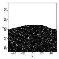
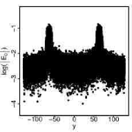
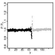
TSPH-CS-128

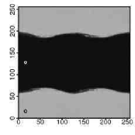
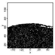
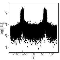
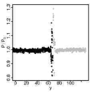
TSPH-CT-128

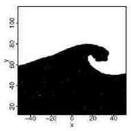
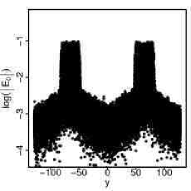
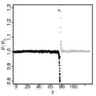
TSPH-HOCT4-442

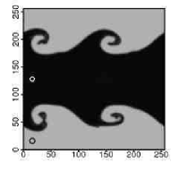
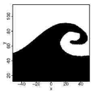
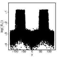
OSPH-HOCT4-442

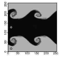
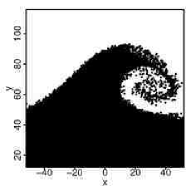
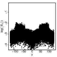
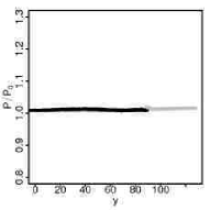
Figure 4: A Kelvin-Helmholtz instability (density ratio $R_{\rho}=2$) at $\tau_{\mathrm{KH}}=1$ modelled with SPH, TSPH and OSPH using CS, CT and HOCT4 kernels (see equations 44, 45 and 46). From left to right the plots show, in a slice of width $dx=1$ about the z-axis: density contours; a zoom-in on the particle distribution around one of the rolls; the magnitude of the $|{\bf E}_{0}|$ error (see equation 28) as a function of $y$; and the pressure in a slice of width $dx=1$ about the x-axis, as a function of $y$. The circles on the density contour plots mark the size of the smoothing kernel, $h$.

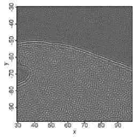
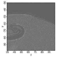
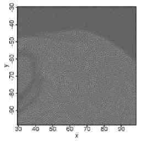
Figure 5: A zoom in on the boundary for the KH test in (from left to right): TSPH-CT-128, TSPH-HOCT4-442 and OSPH-HOCT4-442 at $\tau_{\mathrm{KH}}=1$. The plots are vertical projections of all the points within a $64\times 64\times z$ cuboid. Each point is plotted as a solid black circle with some transparency in order for the gaps to stand out.

TSPH-CT-128

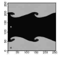
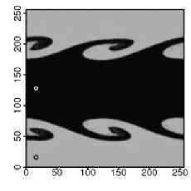
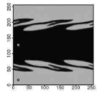
TSPH-HOCT4-442

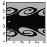
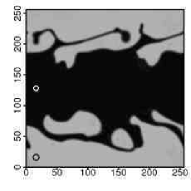
OSPH-HOCT4-442

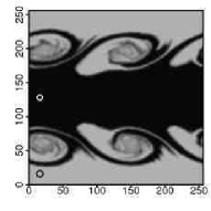
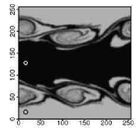
OSPH-HOCT4-442; 1:8 density ratio

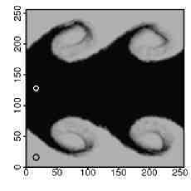
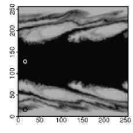
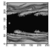
RAMSES; $256\times 256$ cells, no refinement, LLF Riemann solver

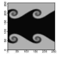
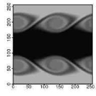
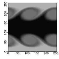
Figure 6: Long term evolution of the KH instability in TSPH and OSPH versus the Eulerian code RAMSES. From left to right, the panels show density contours in a slice of width $dx=1$ about the z-axis at times $\tau_{\mathrm{KH}}=1,2$ and 3.

SPH-CS-442

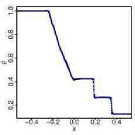
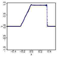
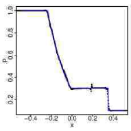
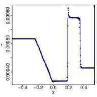
OSPH-HOCT4-442

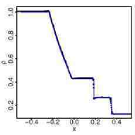
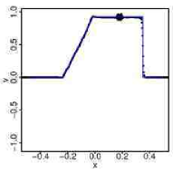
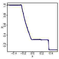
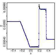
Figure 7: A Sod shock tube test in SPH (top) and OSPH (bottom). From left to right the panels show the variation in density, velocity, pressure and temperature across the shock, respectively. The blue lines give the analytic solution. This test was performed in 3D.

SPH-CS-32; 31,686 particles in the blob
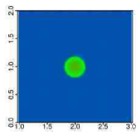
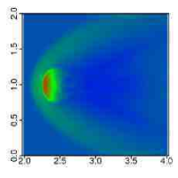
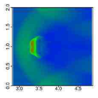
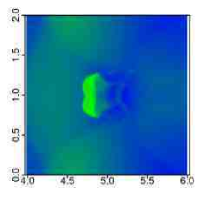
TSPH-HOCT4-442; 126,744 particles in the blob
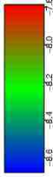
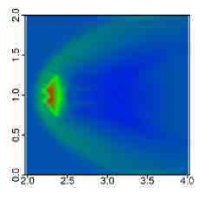
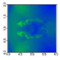
                       OSPH-HOCT4-442; 126,744 particles in the blob
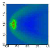
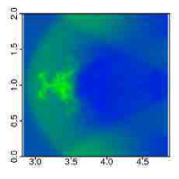
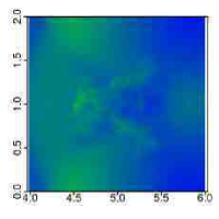
                                 FLASH; $128\times 128\times 384$, 8785 cells in the blob, no refinement
                                

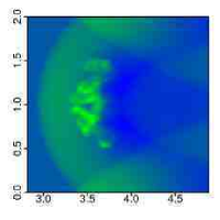
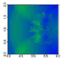
Figure 8: The blob test in SPH, TSPH, OSPH and the Eulerian code FLASH. From left to right the plots show density contours at times $\tau_{\mathrm{KH}}=0,1,2$ and 3. The contour bar gives logarithmic density in cgi units.

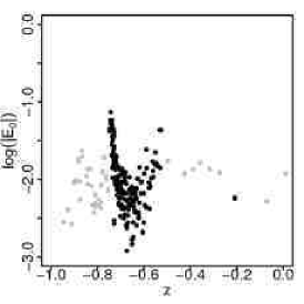
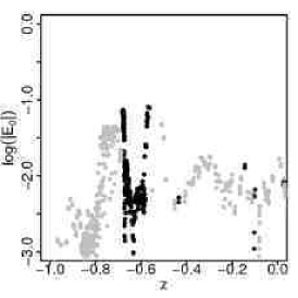
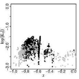
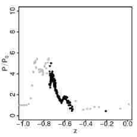
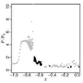
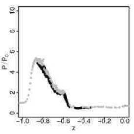
Figure 9: The magnitude of the $|{\bf E}_{0}|$ error in a slice of width $dx=1$ about the z-axis, as a function of $y$ (top); and the pressure in a slice of width $dx$ about the x-axis and $dx$ about the z-axis, as a function of $y$ (bottom) for the blob test in SPH-32 (left), TSPH-HOCT4-442 (middle) and OSPH-HOCT4-442 (right) at time $\tau_{\mathrm{KH}}=1$.

The clumping instability is a problem because it means that increasing the neighbour number will not give improved sampling of the kernel, and the ${\bf E}_{0}$ error will remain large. However, the situation is dramatically improved if we add a constant central core to the kernel gradient $\frac{\partial W}{\partial r}$. This gives a constant force term at the centre of the Kernel that physically prevents clumping. We choose a kernel that is maximally similar to the CS kernel, while obeying $\frac{\partial W}{\partial r}=\mathrm{const.}$ $\forall r<\alpha$, where $\alpha$ is the core size. This leads us to the Core Triangle (CT) kernel:

$$W=\frac{N}{h^{3}}\left\{\begin{array}[]{lr}\left(-12\alpha+18\alpha^{2}\right)x+\beta&0<x\leq\alpha\\ 1-6x^{2}+6x^{3}&\alpha<x\leq\frac{1}{2}\\ 2(1-x)^{3}&\frac{1}{2}<x\leq 1\\ 0&\mathrm{otherwise}\end{array}\right.$$ (45)

where $\beta=1+6\alpha^{2}-12\alpha^{3}$, $N=8/[\pi\left(6.4\alpha^{5}-16\alpha^{6}+1\right)]$, and the core size is fixed at $\alpha=1/3$ by the requirement that $\frac{\partial^{2}W}{\partial r^{2}}$ be continuous.

Figure 2 shows stability plots for the CT kernel. The CT kernel has greatly improved stability for the longitudinal waves (top row) compared to the CS kernel and should give significantly improved performance for large neighbour number. We demonstrate this in §5.

Note that for all of the kernels we use in this paper, we consistently apply the kernel for the density estimate and its gradient for the energy and momentum equations. For small neighbour number, the central triangle in the CT kernel will degrade the quality of the density estimate. However, in this paper we typically use large neighbour numbers ($>100$). In this case, very few particles sample the inner regions of the kernel and the bias introduced in the density is negligible. (The quality of the density estimate in OSPH can be seen in the Sod shock tube test in §6.) We found in tests that retaining the CS kernel just for the density estimate gives near-identical results.

3.4.2 The banding instability

The clumping instability is a result of unstable longitudinal waves. A related instability – the banding instability – is a result of unstable transverse waves. For both the CT and CS kernels, there are broad bands of instability to transverse waves (see Figures 1 and 2). If the neighbour number is carefully chosen to lie in a stable region, banding will not occur. However, banding can still be excited at boundaries if $h$ changes there, moving into an unstable region.

For both the CS and CT kernels, it is difficult to find a suitable neighbour number for which the kernel is stable to all transverse and longitudinal modes. This suggests hunting for an even more stable kernel. A full search is beyond the scope of this paper. Here, we present a simple class of kernels that improve stability by moving to higher order (Morris, 1996b). Following Price (2005), we generalise our CT kernel to order $n_{k}$ to obtain the following class of kernels that we call the High Order Core-Triangle (HOCT) kernels:

$$W=\frac{N}{h^{3}}\left\{\begin{array}[]{lr}Px+Q&0<x\leq\alpha\\ (1-x)^{n_{k}}+A(\gamma-x)^{n_{k}}+&\alpha<x\leq\beta\\ B(\beta-x)^{n_{k}}&\\ (1-x)^{n_{k}}+A(\gamma-x)^{n_{k}}&\beta<x\leq\gamma\\ (1-x)^{n_{k}}&\gamma<x\leq 1\\ 0&\mathrm{otherwise}\end{array}\right.$$ (46)

where:

$$A=\frac{1-\beta^{2}}{\gamma^{n_{k}-3}(\gamma^{2}-\beta^{2})}$$ (47)

$$B=-\frac{1+A\gamma^{n_{k}-1}}{\beta^{n_{k}-1}}$$ (48)

$$P=-n_{k}(1-\alpha)^{n_{k}-1}-n_{k}A(\gamma-\alpha)^{n_{k}-1}-n_{k}B(\beta-\alpha)^{n_{k}-1}$$ (49)

$$Q=(1-\alpha)^{n_{k}}+A(\gamma-\alpha)^{n_{k}}+B(\beta-\alpha)^{n_{k}}-P\alpha$$ (50)

and $\alpha$ and $N$ are calculated numerically for a given choice of $n_{k}$. Continuity requires that $\alpha$ solves the equation:

$$0=(1-\alpha)^{n_{k}-2}+A(\gamma-\alpha)^{n_{k}-2}+B(\beta-\alpha)^{n_{k}-2}$$ (51)

where $\beta$ and $\gamma$ are free parameters. In this paper we choose $\beta=0.5,\gamma=0.75$. Other choices, and indeed other high-order kernels, may give better results than those presented here. We tabulate values for $A,B,P,Q,\alpha$ and $N$ as a function $n_{k}$ in Table LABEL:tab:hoctkern. Notice that the core size $\alpha$ decreases with $n_{k}$.

Stability plots for the HOCT4 kernel (with $n_{k}=4$) are given in Figure 3. Notice the improvement over the CT kernel, particularly for the transverse waves. There are two bands where the kernel is fully stable to both longitudinal and transverse waves on a lattice: 96 neighbours and 442 neighbours, corresponding to $h=2.86$ and $h=4.75$, respectively. We use the latter choice since this also gives very low ${\bf E}_{0}$. The CT kernel also has a stability band for $h\sim 4.75$, but this is narrower than for the HOCT4 kernel, while the HOCT4 kernel with this many neighbours gives better spatial resolution. (It is important to realise that the smoothing length for different kernels takes on a different meaning in terms of spatial resolution. We suggest a resolution criteria based on the numerical sound speed versus the true sound speed for longitudinal waves: $\omega^{2}/k^{2}/c_{s}^{2}$. Spatial scales are well resolved if $\omega^{2}/k^{2}/c_{s}^{2}\simeq 1$. By this definition, our choice of 442 neighbours ($h=4.75$) for the HOCT4 kernel gives a very similar spatial resolution to 128 neighbours ($h=3.14$) for the CT kernel.)

Note that our stability analysis only applies for particles arranged on a lattice. Hexagonal close-packed particles, randomly arranged particles, and indeed boundaries may have different preferred stability regions. A full analysis is beyond the scope of this present work.

The banding instability is not as problematic as the clumping instability for the tests we present in §5 and §7. Unlike the clumping instability, it does not seem to (directly) play a major role in preventing mixing from occurring in SPH (see §5.2.2).

Table 1: Parameters for a selection of High Order Core-Triangle (HOCT) kernels. See equation 46 for details and definitions.

$n_{k}$	$A$	$B$	$P$	$Q$	$\alpha$	$N$
3	2.4	-9.4	-1.81	1.028	0.317	3.71
4	3.2	-18.8	-2.15	0.98	0.214	6.52
5	4.27	-37.6	-2.56	0.962	0.161	10.4
8	10.1	-300.8	-3.86	0.942	0.0927	30.75

3.5 The local mixing instability & RT densities

Our error analysis in §3.3 missed one very important error term. This is because the Taylor expansion assumed that both the pressures and velocities in the flow are smooth. Unfortunately, in SPH at sharp boundary this is not the case. The reason for this is easiest to understand using the entropy form of SPH, as follows (similar arguments apply also for the energy form).

Imagine a density step of ratio $R_{\rho}=\rho_{1}/\rho_{2}$ initially in pressure equilibrium, such that the entropy function (equation 22) is given by $A_{1}/A_{2}=1/R_{\rho}^{\gamma}$. Now imagine that we perturb the boundary very slightly by pushing a low density particle towards it. The particle’s entropy is conserved, but its density increases very rapidly proportional to $R_{\rho}$. This leads to an increase in pressure: $P_{1}=P+\kappa_{1}R$, where $\kappa_{1}$ is some constant that depends on the perturbation size and the kernel. On the other side of the boundary, if we push a high density particle towards the low density region, however, its density will rapidly decrease giving a decrease in pressure: $P_{2}=P-\kappa_{2}R_{\rho}$. This drives us towards a pressure discontinuity at the boundary which drives an associated error in the momentum equation. It can be thought of as a fundamental result of particles trying to mix on the kernel scale, but being unable to as a result of entropy conservation. We call this the local mixing instability (LMI).

Although not phrased in terms of the LMI, the LMI is a recognised problem in the literature and there are essentially two classes of solution. We can generate entropy at the boundary to give smooth entropies and therefore smooth pressures, as in (Wadsley et al., 2008) and Price (2007); or we can try to obtain sharper densities that are consistent with the discrete entropies. This is the approach adopted by Ritchie & Thomas (2001), and the approach we take in this paper. The key advantage of sharpening the densities is that we do not need to specify a subgrid mixing model.

The sharper densities we require are exactly what we get from the density estimate given in equation 36, and originally proposed by Ritchie & Thomas (2001) – the ‘RT’ density estimate. Consider the perturbation discussed above, but now using the RT density estimate. A low density particle which has half of its kernel in the high density phase (an extreme example), will have a density:

$$\rho_{\mathrm{low}}=\sum_{j}^{N_{l}}m_{j}\overline{W}_{ij}+\sum_{j}^{N_{r}}\left(\frac{A_{j}}{A_{i}}\right)^{\frac{1}{\gamma}}m_{j}\overline{W}_{ij}$$ (52)

where $N_{l}$ is the number of particles in the low density region, $N_{r}$ is the number in the high density region, and we have used the fact that the ratio $\left(A_{j}/A_{i}\right)^{\frac{1}{\gamma}}=1$ for the low density region.

If the simulation is adiabatic and started in pressure equilibrium, then for the high density region $\left(A_{j}/A_{i}\right)^{\frac{1}{\gamma}}=1/R_{\rho}$, and since the high density particles sample the kernel $R_{\rho}$ times more often than the low density particles, we recover:

$$\rho_{\mathrm{low}}=\sum_{j}^{N}m_{j}\overline{W}_{ij}$$ (53)

which is identical to a particle in the low density region. A similar derivation applies to a high density particle at the boundary. Thus, the RT density estimate ensures that densities remain sharp. It is straightforward to show that it also ensures the pressures are single valued throughout the flow. Substituting the RT density estimator (equation 36) into equation 22, we obtain:

$$P_{i}=\left[\sum_{j}^{N}m_{j}A_{j}^{\frac{1}{\gamma}}\overline{W}_{ij}\right]^{\gamma}$$ (54)

Notice that the entropy function $A_{j}$ now appears inside the sum, whereas in standard SPH it would appear as $A_{i}$ outside of the sum. This difference ensures that the $P_{i}$ will be everywhere single valued throughout the flow – even at boundaries. A similar derivation can be made for the energy form of SPH, in which case we should use the density estimate given in equation 35.

The RT density estimate is robust to particle mixing on the kernel scale and should lead to a dramatically reduced LMI. We demonstrate this in §5. Furthermore, the RT density estimate ensures that our error analysis in §3.3 is valid by construction since it ensures smooth pressures (recall that we assumed that both the pressures and the velocities were smooth, but not the densities). And, since the RT density estimate leads to sharper densities, it gives improved volume estimates for the particles. This suggests that we can expect the RT density estimate to reduce ${\bf E}_{0}$ at boundaries. We demonstrate this also in §5.

Note that the RT density estimate is chosen to ensure single valued pressures throughout the flow. However, when extracting results from a simulation, it is the positions of the particles themselves that describe the state of the fluid. This suggests using the density estimate in equation 1 for calculating the observable flow density, rather than the RT density estimate. This is the approach we adopt in this paper, though the difference is negligible.

4 Implementation

We implemented OSPH in the GASOLINE code (Wadsley et al., 2004), a parallel implementation of TreeSPH that uses a fixed number $N$ of smoothing neighbours, and a standard prescription for the artificial viscosity as in Gingold & Monaghan (1983) with $\alpha=1$, $\beta=2$, controlled with a Balsara switch (Balsara, 1989). We used variable timesteps controlled by the Courant time with a Courant factor of $0.4$.

The improved stability and error properties of OSPH motivate a full re-examination of the standard SPH artificial viscosity. This is beyond the scope of this present work. However, we note that the improved stability in OSPH means that particles better follow characteristics of the flow, while the gradients in the Balsara switch will be less noisy. Both of these effects should act to decrease the viscosity in regions of steady flow. (Note that all numerical schemes carry numerical viscosity, whether it is manifested through limited resolution or artificial shock-capturing viscosity. Indeed, these viscous terms are vital for successfully modelling shocks.) In §5, §6 and §7, we show that our OSPH results agree very well with analytic expectations, and with the results from Eulerian codes. This suggests that the viscosity prescription in OSPH is not a significant source of error. Certainly it is not responsible for SPH’s inability to model mixing processes.

5 The Kelvin-Helmholtz instability

In this section, we use a 1:2 and 1:8 density ratio shearing fluid simulation to test mixing in OSPH. We use the naming convention XSPH-K-N, where X denotes the variety of SPH, K the choice of kernel, and N the neighbour number (see Table 2).

Flavour of SPH	$\eta$	$\phi$	$\zeta$	Kernel
SPH	1	1	1	CS
TSPH	1	$\rho$	1	CS, CT, HOCT4
OSPH	1/u	$\rho$	1/u	HOCT4

Table 2: The different flavours of SPH we explore in this work. The free functions $\eta,\phi$ and $\zeta$ are defined in equations 16, 17 and 18. The Cubic Spline (CS) kernel is given by equation 44, the Core-Triangle (CT) kernel is given by equation 45, and the fourth order High-Oder Core Triangle (HOCT4) kernel is given by equation 46 with $n_{k}=4$.

5.1 Numerical set-up

A Kelvin-Helmholtz instability (KHI) occurs when two shearing fluids are subjected to an infinitesimal perturbation at the boundary layer. The result of the perturbation is a linearly growing phase in which the layers start to interpenetrate each other, progressively developing into a vortex in the non-linear phase that mixes the two fluid layers. The growth-rate of the instability is in general a complicated function of the shear velocity, fluid densities, compressibility, interface thickness, gravity, viscosity, surface tension, magnetic field strength etc. In this test, we are only interested in the behaviour of inviscid, incompressible (i.e. with bulk motions very much less than the sound speed) perfect fluids neglecting gravity. In this case, the linear growth rate of the KHI is (Chandrasekhar 1961):

$$w=k\frac{(\rho_{1}\rho_{2})^{1/2}v}{(\rho_{1}+\rho_{2})},$$ (55)

where $k=2\pi/\lambda$ is the wavenumber of the instability, $\rho_{1}$ and $\rho_{2}$ are the densities of the respective layers and $v=v_{1}-v_{2}$ is the relative shear velocity. The characteristic growth time for the KHI is then:

$$\tau_{\rm KH}\equiv\frac{2\pi}{w}=\frac{(\rho_{1}+\rho_{2})\lambda}{(\rho_{1}\rho_{2})^{1/2}v}.$$ (56)

This is a particularly challenging test for SPH/OSPH because the velocity due to particle noise can approach the sound speed which can wash out the physical velocity perturbation relevant for this test.

For the simulations, we set up the problem in three dimensions using a periodic thin slab defined by $x\in\{-0.5,0.5\}$, $y\in\{-0.5,0.5\}$ and $z\in\{-1/64,1/64\}$. The domain satisfied:

$$\rho,T,v_{x}=\left\{\begin{array}[]{rl}\rho_{1},T_{1},v_{1}&|y|<0.25\\ \rho_{2},T_{2},v_{2}&|y|>0.25\end{array}\right.$$ (57)

The density and temperature ratio were $R_{\rho}=\rho_{\rm 1}/\rho_{\rm 2}=T_{\rm 2}/T_{\rm 1}=c_{\rm 2}^{2}/c_{\rm 1}^{2}$, ensuring that the whole system was pressure equilibrium. The two layers were given constant and opposing shearing velocities, with the low density layer moving at a Mach number $\mathcal{M}_{\rm{2}}=-v_{\rm 2}/c_{\rm 2}\approx 0.11$ and the dense layer moving at $\mathcal{M}_{\rm{1}}=\mathcal{M}_{\rm{2}}\sqrt{R_{\rho}}$. The density ratios considered in this work are small which assures a subsonic regime where the growth of instabilities can be treated using equation 56 (Vietri et al., 1997).

To trigger instabilities, velocity perturbations were imposed on the two boundaries of the form:

$$v_{y} = \delta v_{\rm y}[\sin(2\pi(x+\lambda/2)/\lambda)\exp(-(10(y-0.25))^{2})$$ (58)

$$-\sin(2\pi x/\lambda)\exp(-(10(y+0.25))^{2})]$$

where the perturbation velocity $\delta v_{\rm y}/v=1/8$ and $\lambda=0.5$ is the wavelength of the mode.

Equal mass particles were placed in lattice configurations to satisfy the setup described above. To satisfy pressure equilibrium everywhere, in TSPH the temperatures were adjusted at boundaries to be coherent with the smoothed density step measured by equation 1. This was not done for the OSPH simulations since these sharpen the densities using the discrete initial temperatures.

The low density region $\rho_{2}$ was set up using 256 particles in the $x$-direction and the appropriate number of particles in the other dimensions to satisfy a fixed inter-particle distance. The high density region $\rho_{1}$ was created in the same way with 320 particles in the $x$-direction. We adopted a periodic simulation domain.

The RAMSES simulation used the same numerical set-up as described above, but in 2D rather than in a thin slab. We performed the $R_{\rho}=2$ simulation using the LLF Riemann solver (Toro, 1999) on a $256\times 256$ fixed Cartesian grid. The LLF solver is rather diffusive and is used in order to suppress the growth of undesirable small scale KHIs arising from grid irregularities.

We note that all numerical schemes carry numerical viscosity, whether it is manifested through limited resolution or artificial shock-capturing viscosity. A detailed study of this effect on the KHI and the relation to physical viscosity is beyond the scope of this paper.

5.2 Results

Figure 4 shows our results for the KHI test (density ratio $R_{\rho}=2$) at $\tau_{\mathrm{KH}}=1$ modelled with SPH, TSPH and OSPH, using three different kernels: CS, CT and HOCT4, and different neighbour numbers as marked on each plot (see also Table 2). From left to right, the panels show, in a slice of width $dx=1$ about the z-axis: density contours of the simulation box, a zoom in on the particle distribution around on of the rolls, the magnitude of the $|{\bf E}_{0}|$ error (equation 28) as a function of $y$, and the pressure as a function of $y$ in a slice of width $dx=1$ about the x-axis.

5.2.1 The clumping instability

Using the standard CS kernel, SPH-CS-128 (top row, Figure 4) and TSPH-CS-128 (second row) give poor results that improve very slowly with increasing neighbour number. This can be seen both in the lack of strong evolution on the boundary, and in the large $|{\bf E}_{0}|$ error, even for 128 neighbours. TSPH-CS-128 gives slightly better results than SPH-CS-128, showing the first beginnings of a KHI roll, but both are in poor agreement with the RAMSES results (bottom row).

The reason for the poor performance in both SPH-CS-128 and TSPH-CS-128 is the clumping instability (§3.4.1). Particles gather together on the kernel scale, giving poor kernel sampling, and poor associated error. This can be seen in the particle distribution for SPH-CS-128 and TSPH-CS-128 (second row, Figure 4) which show visible holes and over-densities in the particle distribution. Using instead the CT kernel introduced in §3.4.1, the results improve dramatically (third row, Figure 4). Now the errors reduce for increasing neighbour number (see Appendix A). With 128 neighbours, we successfully resolve a KH roll up to $\tau_{\mathrm{KH}}=1$ with the correct growth time.

It has been noted previously in the literature that putting a small core inside a cubic spline kernel suppresses the clumping instability (Thomas & Couchman 1992; Herant 1994), though its importance for modelling multiphase flow was not realised. Alternative fixes include adding an negative pressure term (Monaghan, 2000), which in tests we find works also. However, we prefer changing the kernel to introducing new forces since we may then still estimate our errors through $|{\bf E}_{0}|$.

5.2.2 The banding instability

In addition to the clumping instability, there is also an instability to transverse waves – the banding instability (§3.4.2). For the KHI tests we present here, the banding instability occurs only on the boundary and appears to be relatively benign. This is shown in Figure 5, that shows a zoom in on the boundary at $\tau_{\mathrm{KH}}=1$ for TSPH-CT-128, TSPH-HOCT4-442 and OSPH-HOCT4-442. The TSPH-CT-128 simulation has a kernel and neighbour number combination that are unstable to transverse waves (see Figure 2), and banding is clearly visible on the boundary. However, TSPH-HOCT4-442 should be stable to transverse waves, yet the banding persists. Only in our full scheme, OSPH-HOCT4-442, is the banding is gone.

To understand the above results, we ran an additional test that we omit for brevity – TSPH-HOCT4-96. This simulation showed little boundary evolution because the low neighbour number and associated large $|{\bf E}_{0}|$ significantly damped the KHI. However, interestingly, there was no banding observed on the boundary (recall that 96 neighbours for the HOCT4 kernel should be stable to both transverse and longitudinal wave perturbations).

Taken together, our results suggest that the observed banding at the boundary is a result of a transverse wave instability driven by the local mixing instability (LMI; §3.5). Where there is little evolution at the boundary and the kernel is chosen to be stable to transverse waves, the banding disappears, as was the case for our extra TSPH-HOCT4-96 simulation. Where there is strong evolution at the boundary, as was the case for TSPH-HOCT4-442, the LMI drives banding irrespective of the choice of kernel. Only in our full scheme, OSPH-HOCT4-442, where the LMI is cured and the kernel is stable to transverse waves, is the banding cured.

5.2.3 The ${\bf E}_{0}$ error

Away from boundaries, the ${\bf E}_{0}$ error in TSPH decreases with the neighbour number, as expected for smooth flow (see Appendix A). However, on the boundary the $|{\bf E}_{0}|$ error grows by 2-3 orders of magnitude. Increasing the neighbour number does result in better long-term evolution, but the results improve very slowly. This is shown in Figure 6. Notice that TSPH-HOCT4-442 resolves two wraps of the KH roll at $\tau_{\mathrm{KH}}=2$, whereas TSPH-CT-128 only manages one. However, even in TSPH-HOCT4-442, the long-term evolution eventually degrades. By $\tau_{\mathrm{KH}}=3$, the results are ‘gloopy’, rather similar to simulations that explicitly model fluid surface tension (see e.g. Herrmann 2005).

The poor ${\bf E}_{0}$ on the boundary is the result of a poor volume estimate for each particle $m_{j}/\rho_{j}$ (see §3.3). However ${\bf E}_{0}$ is not solely responsible for the gloopy behaviour. There is a second problem – similar to a numerical surface tension term – that needs to be solved extra to minimising ${\bf E}_{0}$. This is the local mixing instability (LMI) error (§3.5).

5.2.4 The local mixing instability error

The right panels of Figure 4 show the pressure as a function of $y$ in a slice of width $dx=1$ about the z-axis and width $dx=1$ about the x-axis. In SPH and TSPH  there is a clear pressure discontinuity on the boundary. This is caused by the local mixing instability (LMI) discussed in §3.5.

Notice that the pressure blip is larger in TSPH than in SPH, yet the KHI roll progresses further in TSPH than in SPH. This apparent paradox is the result of the improved performance in TSPH. As the KHI roll progresses in TSPH, particles are pushed closer to the boundary making the LMI worse and increasing the pressure blip. In SPH, there is a larger gap at the boundary due to the larger surface tension error. This leads to less evolution and a smaller associated pressure blip. We will see a similar effect occurring in the blob test in §7.

As discussed in §3.5, the LMI should be cured by the RT density estimate (equation 35). This is shown in Figure 4, third row which shows the results for our full OSPH scheme. With the RT densities, the pressure at the boundary has a much smaller blip, while ${\bf E}_{0}$ is reduced by over an order of magnitude. This latter effect occurs since the RT densities also give an improved volume estimate for each particle (see §3.3 and §3.5). The long term evolution is now in excellent agreement with the RAMSES results (compare Figure 4 third and bottom rows).

Although OSPH gives significantly improved results as compared with SPH, the scheme is numerically expensive. Simulations with larger density gradients require very high resolution. This is shown in Figure 6, second from bottom row. This shows the long term evolution of a KHI test with density ratio $R_{\rho}=8$ in OSPH. The solution should be similar to the $R_{\rho}=2$ simulation, but it is not. The ‘gloopy’ behaviour indicative of large surface tension errors has returned. Further increasing the neighbour numbers would reduce this problem, but at increased numerical cost. We will address this issue in future work (Hayfield & Read in prep.).

6 The Sod shock tube

Before we embark on the blob test in §7, it is worth checking that our new OSPH scheme can still correctly resolve shocks. To test this, we use a standard Sod shock tube test (Sod, 1978).

The Sod shock tube consists of a 1D tube on the interval $[-0.5,0.5]$ with a discontinuous change in properties at $x=0$ designed to generate a shock. The left state is described by $\rho_{l}=1.0$, $P_{l}=1.0$, $v_{l}=0$, and the right state by $\rho_{r}=0.125$, $P_{r}=0.1$, $v_{r}=0$, where $\rho,P$ and $v$ are the density, pressure and velocity along the $x$ axis. We use an adiabatic equation of state with $\gamma=1.4$. The subsequent evolution of the problem has a self-similar analytic solution that has a number distinct features which quite generally test a code’s conservation properties, artificial viscosity, ability to handle nonlinear waves, and shock resolution.

Figure 7 shows the results for the Sod shock tube test at time $t=0.2$ in SPH (top) OSPH (bottom). Since we are primarily concerned with the 3D performance of the code, the test was performed in 3D on the union of a $24\times 24\times 300$ lattice on the left, with a $12\times 12\times 150$ lattice on the right, giving a 1D resolution of 450 points. We use 442 neighbours for this test in both SPH and OSPH to ensure that any difference is not simply due to improved kernel sampling in OSPH.

For SPH, the only strong disagreement with the analytic solution is in the pressures that have a blip at $x=0.2$, and the temperatures that overshoot at $x=0.2$. The former feature is due to the LMI (see §3.5 and §5.2.4). The latter feature is seen in all SPH Sod shock tube tests and results from the well-known ‘wall heating’ effect (Noh, 1987). This is an error due to the artificial viscosity prescription and is beyond the scope of this present work.

For OSPH, the results are even better than for SPH. The pressure blip is now gone, while the temperature overshoot at $x=0.2$ is reduced. Only the velocities appear to be worse, with some remaining dispersion at $x=0.2$. This owes to the jump in density at this point, and the associated jump in $|{\bf E}_{0}|$. This gives a force error at the discontinuity which introduces some dispersion into the velocities. In SPH this cannot occur since the LMI causes a pressure blip at the boundary that prevents mixing. We will discuss this issue further in a forthcoming paper (Hayfield & Read in prep.).

7 The blob test

The KHI test presented in §5 is a worst-case scenario for OSPH, since it has a pure adiabatic sharp boundary. For many practical situations, boundaries will be less sharp, while physical entropy generation due to shocks and/or cooling will suppress the LMI. We give a practical example of this in this section using the blob test described in Agertz et al. (2007). A spherical cloud of gas of radius $R_{\rm cl}$ is placed in a wind tunnel with periodic boundary conditions. The ambient medium is ten times hotter and ten times less dense than the cloud so that it is in pressure equilibrium with the latter. We refer to the initial density contrast between the cloud and the medium as $R_{\rho,{\rm ini}}$. The wind velocity ($v_{\rm wind}=c_{s}\mathcal{M}$) has an associated Mach number $\mathcal{M}=2.7$. This leads to the formation of a bow shock after which the post-shock subsonic flow interacts with the cloud and turns supersonic as it flows past it.

The blob test is useful for investigating how different hydrodynamics codes model astrophysical processes important for multiphase systems, such as shocks, ram-pressure stripping and fragmentation through KH and Rayleigh-Taylor (RT) instabilities. As $\tau_{\rm KH}<\tau_{\rm RT}$, an approximate timescale of the cloud destruction is that of the full growth of the largest KH mode, i.e. the wavelength of the cloud’s radius. This can be obtained by considering the post-shock flow on the cloud and its time-dependence as the shock weakens and the cloud is accelerated. A full analysis of this test is presented in Agertz et al. (2007) and gives $\tau_{\rm KH}\approx 1.6\tau_{\rm cr}$ where $\tau_{\rm cr}=2R_{\rm{cl}}R_{\rho,{\rm ini}}^{1/2}/v$ is the crushing time and the velocity $v$ refers to the streaming velocity in the reference frame of the cloud. After this time, the cloud is expected to show a more complicated non-linear behaviour leading to disruption. The original blob test was initialised in a glass-like configuration obtained using simulated annealing using a standard SPH code. Since we now use OSPH rather than SPH, we must set up new ICs for the blob. Our new IC set up is described in detail in Appendix B. Unlike the previous blob test, where perturbations were seeded by random noise in the particle distribution, here we deliberately seed an inward growing mode on the front surface of the blob. This makes comparison between OSPH and FLASH simpler, since then the morphology of the blob is less dependent on small scale numerical noise.

The results are presented in Figure 8, where we compare SPH, TSPH and OSPH with increasing resolution with similar results from the Eulerian code FLASH (Fryxell et al., 2000). The SPH results (top panels) are similar to those presented in Agertz et al. (2007). The blob is squashed by the shock, but does not break up. There are no visible surface KHI or Rayleigh-Taylor instabilities. TSPH (second row) gives significantly improved results. The central depression is now resolved and the blob is mostly destroyed by $\tau_{\rm KH}=3$. However, the density remains clumpy as compared to the FLASH simulation (bottom row). Our full OSPH scheme (third row) gives excellent agreement with the FLASH results. There are clear surface KHI and RT instabilities and the blob breaks up fully by $\tau_{\rm KH}=3$. The precise details of the break up in FLASH and OSPH are different. However, these differences are smaller than those we observed between FLASH simulations of varying resolution. They are caused by the non-linear break up of the blob that is affected by resolution-scale perturbations.

Figure 9 shows ${\bf E}_{0}$ and the pressure blips for the blob test in SPH (left), TSPH (middle) and OSPH (right) at $\tau_{\rm KH}=1$. In SPH and TSPH, the two fluid phases (marked by the black and grey solid circles) remain well separated at all times. In both cases the pressure distribution shows discontinuities. By contrast, in OSPH the fluids are already mixed at $\tau_{\rm KH}=1$, while the pressures are smooth and single-valued throughout the flow.

There is a more modest improvement in ${\bf E}_{0}$ between SPH, TSPH and OSPH than that seen in the KHI tests presented in §5. OSPH gives a ${\bf E}_{0}$ smaller by a factor $\sim 5$ compared to the SPH and TSPH simulations, whereas in the KHI tests, there was an improvement of over an order of magnitude. There are two reasons for this. Firstly, since the SPH simulation shows little evolution at the boundary, the initial ${\bf E}_{0}$ is relatively well conserved. By contrast, TSPH shows significant boundary evolution due to improved mixing. This can actually worsen ${\bf E}_{0}$ at the boundary since the particles are still unable to properly interpenetrate as a result of the LMI. Figure 8 clearly shows, however, that TSPH gives improved mixing. Secondly, entropy generation at the shock softens the density step around the blob, leading to an improved ${\bf E}_{0}$ even for the SPH simulation.

8 Conclusions

Standard formulations of smoothed particle hydrodynamics (SPH) cannot resolve fluid mixing and instabilities at flow boundaries. We have used an error and stability analysis of the generalised SPH equations of motion to show that mixing fails for two distinct reasons. The first is a leading order error in the momentum equation. This should decrease with increasing neighbour number, but does not because numerical instabilities cause the kernel to be irregularly sampled. We identified two important instabilities: the clumping instability and the banding instability, and we showed that both are cured by a suitable choice of kernel. The second problem is the local mixing instability (LMI). This occurs as particles attempt to mix on the kernel scale, but are unable to due to entropy conservation. The result is a pressure discontinuity at boundaries that pushes fluids of different entropy apart. We cured the LMI by using a weighted density estimate proposed by Ritchie & Thomas (2001). We showed that this both reduces errors in the continuity equation and allows individual particles to mix at constant pressure.

We demonstrated mixing in our new Optimised Smoothed Particle Hydrodynamics (OSPH) scheme using a Kelvin Helmholtz instability (KHI) test with density contrast 1:2, and the ‘blob test’ – a 1:10 density ratio gas sphere in a wind tunnel – finding excellent agreement between OSPH and Eulerian codes.

OSPH is a multiphase Lagrangian method that conserves momentum, mass and entropy, and demonstrates that it is possible to model multiphase fluid flow using SPH. However, OSPH remains a low-order method, requiring large neighbour number to keep the ${\bf E}_{0}$ error small. We will address this problem in a forthcoming paper, where we use the lessons learnt in this present work to move to higher order particle methods (Hayfield & Read in prep.).

9 Acknowledgements

We would like to thank the referee Paul Clark for useful comments and suggestions that improved the clarity of this work. We would also like to thank James Wadsley, Walter Dehnen, Joachim Stadel, Romain Teyssier, Volker Springel, Peter Thomas, Peter Englmaier, and Melvyn Davis for useful discussions and comments. J.R. would like to acknowledge support from a Forschungskredit grant from the University of Zürich and an ESF Astrosim grant. The FLASH software used for one of the simulations in this paper was developed by the DOE supported ASCI/Alliances Center for Astrophysical Thermonuclear Flashes at the University of Chicago.

Appendix A The effect of increasing neighbour number in TSPH

In this appendix we show the effect of increasing neighbour number for TSPH-CT (i.e. without the clumping instability). The results for the same KH instability test shown in Figure 4 are shown in Figure 10 for 32 and 64 neighbours. Notice that with increasing particle number, the error vector ${\bf E}_{0}$ is reduced, the pressure blip at the boundary is reduced, and the results improve.

TSPH-CT-32

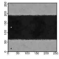
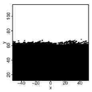
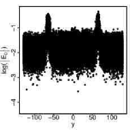
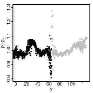
TSPH-CT-64

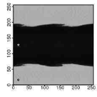
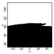
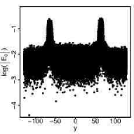
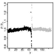
Figure 10: As Figure 4, but showing the effect of increasing particle number for TSPH-CT.

Appendix B The blob test setup

The hydrodynamical properties of the blob test are described in §7. We use a periodic simulation box of size, in units of the cloud radius $R_{\rm cl}$, $\{L_{x},L_{y},L_{z}\}=\{10,10,30\}$ and we centre the cloud at $\{x,y,z\}=\{5,5,5\}$. The equal mass SPH particles constituting the ambient medium and the cloud are arranged in lattice configurations to achieve the relevant density contrast $R_{\rho,{\rm ini}}=10$. The particle temperatures ($T\sim P/\rho$) are then assigned to achieve pressure equilibrium where the local density measurement of equation 1 is used for consistency. The wind velocity ($v_{\rm wind}=c_{s}\mathcal{M}$) has an associated Mach number $\mathcal{M}=2.7$, where the sound speed is $c_{\rm s}=\sqrt{\gamma P/\rho}$ using an adiabatic index $\gamma=5/3$.

In the original blob test described in Agertz et al. (2007), SPH particle noise was used to trigger instabilities. This procedure is not applicable when using a noise free lattice configuration. Hence, we use spherical harmonics to apply large scale perturbations to the surface layer of the cloud. The full perturbation, in spherical coordinates centred on the cloud, can be expressed as $v_{\rm pert}(r,\theta,\phi)=\delta vR(r){\rm Re}[Y(\theta,\phi)_{l}^{m})]/C$, where the radial part, $R(r)=\exp{(2(r-r_{\rm cl})/r_{\rm cl})}$, is defined for $r\leq r_{\rm cl}$ and the spherical harmonic is, adopting $l=5$, $m=3$:

$$Y_{5}^{3}=\frac{-1}{32}\sqrt{\frac{385}{\pi}}e^{3i\phi}\sin^{3}{\theta}(9\cos^{2}{\theta}-1).$$ (59)

The constant $C$ simply normalises the real part of the harmonic to reach a maximum value of 1. We chose a subsonic perturbation $\delta v=-0.06\,v_{\rm wind}$.

References

- Agertz et al. (2007) Agertz O., Moore B., Stadel J., Potter D., Miniati F., Read J., Mayer L., Gawryszczak A., Kravtsov A., Nordlund Å., Pearce F., Quilis V., Rudd D., Springel V., Stone J., Tasker E., Teyssier R., Wadsley J., Walder R., 2007, MNRAS, 380, 963
- Attwood et al. (2007) Attwood R. E., Goodwin S. P., Whitworth A. P., 2007, A&A, 464, 447
- Balsara (1989) Balsara D. S., 1989, PhD thesis, , Univ. Illinois at Urbana-Champaign, (1989)
- Bennett (2006) Bennett A., 2006, Lagrangian fluid dynamics. Cambridge Monographs on Mechanics
- Chandrasekhar (1961) Chandrasekhar S., 1961, Hydrodynamic and hydromagnetic stability. International Series of Monographs on Physics, Oxford: Clarendon, 1961
- Dehnen (2000) Dehnen W., 2000, ApJ, 536, L39
- Dilts (1999) Dilts G., 1999, International journal for numerical methods in engineering, 44, 1115
- Fryxell et al. (2000) Fryxell B., Olson K., Ricker P., Timmes F. X., Zingale M., Lamb D. Q., MacNeice P., Rosner R., Truran J. W., Tufo H., 2000, ApJS, 131, 273
- Gingold & Monaghan (1977) Gingold R. A., Monaghan J. J., 1977, MNRAS, 181, 375
- Gingold & Monaghan (1983) Gingold R. A., Monaghan J. J., 1983, MNRAS, 204, 715
- Goodman & Hernquist (1991) Goodman J., Hernquist L., 1991, ApJ, 378, 637
- Greengard & Rokhlin (1987) Greengard L., Rokhlin V., 1987, Journal of Computational Physics, 73, 325
- Herant (1994) Herant M., 1994, Memorie della Societa Astronomica Italiana, 65, 1013
- Hernquist & Katz (1989) Hernquist L., Katz N., 1989, ApJS, 70, 419
- Herrmann (2005) Herrmann M., 2005, J. Comput. Phys., 203, 539
- Hieber & Koumoutsakos (2008) Hieber S. E., Koumoutsakos P., 2008, Journal of Computational Physics, 227, 9195
- Libersky et al. (1993) Libersky L. D., Petschek A. G., Carney T. C., Hipp J. R., Allahdadi F. A., 1993, Journal of Computational Physics, 109, 67
- Lucy (1977) Lucy L. B., 1977, AJ, 82, 1013
- Maron & Howes (2003) Maron J. L., Howes G. G., 2003, ApJ, 595, 564
- Marri & White (2003) Marri S., White S. D. M., 2003, MNRAS, 345, 561
- Monaghan (1992) Monaghan J. J., 1992, ARA&A, 30, 543
- Monaghan (2000) Monaghan J. J., 2000, Journal of Computational Physics, 159, 290
- Morris (1996a) Morris J. P., 1996a, Publications of the Astronomical Society of Australia, 13, 97
- Morris (1996b) Morris J. P., 1996b, Ph.D. Thesis, Department of Mathematics, Monash University
- Nelson & Papaloizou (1994) Nelson R. P., Papaloizou J. C. B., 1994, MNRAS, 270, 1
- Noh (1987) Noh W., 1987, Journal of Computational Physics, 72, 78
- Oger et al. (2007) Oger G., Doring M., Alessandrini B., Ferrant P., 2007, Journal of Computational Physics, 225, 1472
- Price (2005) Price D., 2005, ArXiv Astrophysics e-prints
- Price (2007) Price D. J., 2007, ArXiv e-prints, 709
- Ritchie & Thomas (2001) Ritchie B. W., Thomas P. A., 2001, MNRAS, 323, 743
- Rosswog (2009) Rosswog S., 2009, New Astronomy Review, 53, 78
- Schuessler & Schmitt (1981) Schuessler I., Schmitt D., 1981, A&A, 97, 373
- Sod (1978) Sod G. A., 1978, Journal of Computational Physics, 27, 1
- Springel (2009) Springel V., 2009, ArXiv e-prints
- Springel & Hernquist (2002) Springel V., Hernquist L., 2002, MNRAS, 333, 649
- Teyssier (2002) Teyssier R., 2002, A&A, 385, 337
- Thomas & Couchman (1992) Thomas P. A., Couchman H. M. P., 1992, MNRAS, 257, 11
- Toro (1999) Toro E. F., 1999, Riemann solvers and numerical methods for fluid dynamics - A practical introduction - 2nd edition. Springer, Berlin
- Vietri et al. (1997) Vietri M., Ferrara A., Miniati F., 1997, ApJ, 483, 262
- Wadsley et al. (2004) Wadsley J. W., Stadel J., Quinn T., 2004, New Astronomy, 9, 137
- Wadsley et al. (2008) Wadsley J. W., Veeravalli G., Couchman H. M. P., 2008, MNRAS, 387, 427