Polarized Fermi gases in asymmetric optical lattices

Abstract

The zero-temperature phase diagrams of imbalanced two-species Fermi gases are investigated in asymmetric optical lattices with arbitrary potential depths, based on the exact spectrum instead of the Fermi-Hubbard model. We study the effect of lattice potentials and atomic densities to the fully paired Bardeen-Cooper-Schrieffer (BCS) state and particularly the Fulde-Ferrell-Larkin-Ovchinnikov (FFLO) state. It is found that the increasing lattice potential favors BCS at low densities because of the enhanced effective coupling; whereas FFLO is favored at intermediate densities when the system undergoes a dimensional crossover. Finally using local density approximation we study the evolution of phase profile in the presence of external harmonic traps by merely tuning the lattice potentials.

I Introduction

Ever since the direct observation of phase separations of unequal two-component ${}^{6}Li$ cold atoms in experimentszwierlein06 ; partridge06 ; zwierlein062 ; shin07 , the topic of polarized Fermi gases has gained enormous interest from theoreticians interests in the past few yearsbedaque03 ; sheehy06 ; hu06 ; parish07np ; wei07 . Such an imbalanced and attractively interacting fermionic system makes it possible to study in the laboratory several exotic fermionic pairing mechanisms, including Sarmasarma63 or breached pairliu03 state and Fulde-Ferrell-Larkin-Ovchinnikov (FFLO) statefflo64 ; yoshida07 with finite pairing momentum. However, it is hard for FFLO state to be experimentally observed in three-dimensional (3D) free space. It was proved to survive in a very small region in the Bardeen-Cooper-Schrieffer (BCS) side of Feshbach resonance and totally vanish in the BEC side, both for a homogeneous Fermi gassheehy06 ; hu06 ; parish07np and a trapped onewei07 . Recently more and more attention has been paid to one-dimensional (1D)huihu07 ; orso07 and two-dimensional (2D)conduit08 systems. It has been pointed out that for these reduced dimensions, the polarization window of FFLO state is generally broadened compared to 3D free space.

Despite many previous studies on imbalanced fermions in pure 1D, 2D and 3D systems, the crossover regimes between different dimensions are poorly understood and still need further investigations, such as quasi-1D and quasi-2D systems. Experimentally, these geometries can be achieved by exposing magnetic or optical traps or optical lattices along selective directions. Among all trapping confinements, optical lattices are the most complicated because of the band structures. A very interesting and important question then immediately arises: How would the dimension and band structure affect the fermionic superfluidity, especially the exotic FFLO state? There have been several works related to this subject. For example, the FFLO state was studied in pure 1D, 2D and 3D optical latices and shown to be enhanced as a result of the Van Hove singularitieskoponen07 ; it was also previously found with evident proportions in an array of 1D tubes produced by 2D optical latticesparish07prl and in two-lag laddersfeiguin09 . In the presence of optical lattices, however, all these studies have adopted the Fermi-Hubbard model based on the tight-binding approximation (TBA), which is generally believed to be valid for deep lattices and not very strong interactions such that the lowest band model is good enough to describe the system. On the other hand, a different approach based on the exact lattice spectrumcui09 shows that TBA does not necessarily produce the correct results because of the multiband effects and deviations of the lowest band structures, even for optical lattices with considerable band gap. In this work we are going to use the exact spectrum to investigate the zero temperature phase diagrams for imbalanced fermions in asymmetric optical lattices, tuned by lattice potential depths and atomic densities. This work studies the FFLO state in optical lattices with arbitrary potential depths. The results obtained reveal the fundamental effects of the dimension and the effective coupling to the strength of fermionic superfluidities, including FFLO state, and thus give an answer to the question previously proposed. Therefore our results can serve as a guideline for cold fermions experiments and might contribute to finally observing the novel FFLO-type pairing state.

In this work we consider optical lattices applied in selective directions and take into account the couplings between different reciprocal lattice vectors, which recently were proved to be necessary for optical latticesmoon07 ; cui09 . The possibility of FFLO pairing is studied in the remanent free direction(s). We find that by increasing the lattice depths, FFLO gradually diminishes at low atomic densities as a result of the enhanced effective coupling, but revives at intermediate densities where the system undergoes a dimensional crossover. Compared with the density-driven BCS-BEC crossover initially studied in exciton superconductorscomte82 and then applied to attractive Fermi gasesNSR85 , the density-driven crossover from weak to strong coupling limits mentioned here is unique to optical lattices and may induce even more significant effects to the system in the sense that it changes the effective dimension. In contrast, the strength of unpolarized BCS superfluidity is enhanced at low atomic densities but frustrated at intermediate ones because of the discontinuity of the energy spectrum. All these results can be understood when investigating the density of state (DOS), which has an intimate and sensitive dependence on the lattice potential and the atomic density. Finally, in the presence of the external harmonic trap, we use local density approximation (LDA) to investigate the evolution of phase profiles merely tuned by the potential depths of asymmetric optical lattices.

The article is organized as follows. In Sec. II we outline our general model and method. In Sec. III we give the phase diagrams for density-imbalanced two-component fermions in several asymmetric optical lattices, including quasi-1D and quasi-2D geometries. We mainly focus on quasi-1D case, which could be achieved by applying optical lattices to either 3D or effective 2D space. The effect of external harmonic confinement is studied in Sec. IV. We summarize our results in the last section.

II General Models

We consider a two-component Fermi gas with contact interactions by the following Hamiltonian

$$H = \int d\mathbf{r}\sum_{\sigma=\uparrow,\downarrow}\psi^{{\dagger}}_{\sigma}(\mathbf{r})\hat{H}_{0}(\mathbf{r})\psi_{\sigma}(\mathbf{r})+$$ (1)

$$g\int d\mathbf{r}\psi^{{\dagger}}_{\uparrow}(\mathbf{r})\psi^{{\dagger}}_{\downarrow}(\mathbf{r})\psi_{\downarrow}(\mathbf{r})\psi_{\uparrow}(\mathbf{r}),$$

where $\hat{H}_{0}=\sum_{i=x,y,z}\hat{H}_{i}$ is composed by the kinetic energy and optical lattice potential if applied; $g$ is the bare contact interaction described by s-wave scattering length $a_{s}$ in 3D as $\frac{1}{g}=\frac{m}{4\pi a_{s}}-\frac{1}{V}\sum_{\mathbf{q}}\frac{1}{2\epsilon_{\mathbf{q}}}$; and by the binding energy $E_{B}$ in effective 2D as $\frac{1}{g}=-\frac{1}{S}\sum_{\mathbf{q}}\frac{1}{2\epsilon_{\mathbf{q}}+E_{B}}$. The renormalization of $g$ here is to eliminate the unphysical divergence due to the high-momentum contribution in a Fermi gas.

To illustrate our scheme, we take a quasi-1D Fermi gas confined by two orthogonal optical lattices in x and y directions. For example, $\hat{H}_{0}=\sum_{i=x,y,z}-\partial_{i}^{2}/2m+V_{0}\big{[}\sin^{2}(\pi x/a)+\sin^{2}(\pi y/a)\big{]}$, here $a$ is the lattice constant and $V_{0}$ the potential depth. By mean-field treatment, first we expand each field operator in terms of eigen-wavefunctions of $\hat{H}_{0}$, $\psi_{\sigma}(\mathbf{r})=\sum_{\mathbf{nk}}\phi_{\mathbf{nk}}(\mathbf{r})\psi_{\mathbf{nk}\sigma}$ with

$$\phi_{{}_{\mathbf{nk}}}(\mathbf{r})=\frac{1}{\sqrt{V}}e^{ik_{z}z}\sum_{\mathbf{G_{\bot}}}a_{{}_{\mathbf{nk_{{}_{\bot}}}}}(\mathbf{G_{\bot}})e^{i(\mathbf{k_{\bot}}+\mathbf{G_{\bot}})\cdot\mathbf{r_{\bot}}},$$ (2)

here $\epsilon_{\mathbf{nk}}=\epsilon^{0}_{k_{z}}+\epsilon_{n_{x}k_{x}}+\epsilon_{n_{y}k_{y}}\ (\epsilon^{0}_{k_{z}}=\frac{k_{z}^{2}}{2m})$ is the eigen-energy; $\mathbf{n}=\big{\{}n_{x},n_{y}\big{\}}$ indicates the band index; $\mathbf{k_{\bot}}$ lies in the first Brillouin Zone ($BZ$) while $k_{z}$ has no constraint; $\mathbf{G_{\bot}}=2\pi/a(l_{x},l_{y})$ is the reciprocal lattice vector. The Bloch wave functions and eigen-energies can be obtained from the decoupled Schrödinger equation in each (x or y) direction

$$\sum_{G^{\prime}}\Big{\{}\big{[}\frac{(k+G)^{2}}{2m}+\frac{V_{0}}{2}\big{]}\delta_{GG^{\prime}}-\frac{V_{0}}{4}\sum_{i}\delta_{G\pm\frac{2\pi}{a},G^{\prime}}\Big{\}}$$

$$\hskip 90.0pt\times a_{nk}(G^{\prime})=\epsilon_{nk}a_{nk}(G),$$ (3)

and the eigenvectors satisfy $\sum_{G}a_{nk}^{*}(G)a_{n^{\prime}k}(G)=\delta_{nn^{\prime}}$ and $a_{n,-k}(-G)=a_{nk}^{*}(G)$. For convenience we rescale the energy and momentum respectively in units of the recoil energy $E_{R}=\frac{1}{2m}(\frac{\pi}{a})^{2}$ and lattice reciprocal vector $\frac{2\pi}{a}$. Then the lattice potential and atomic density are expressed by two dimensionless parameters: $s=\frac{V_{0}}{E_{R}}$ and $n=\frac{Na^{3}}{V}$.

Toward the FFLO state, we employ the simplest single plane wave ansatz to the free direction as $\Delta(\mathbf{r})=\Delta_{q}e^{iqz}$. For the lattice part, however, we focus on the most probable pairing mechanism, i.e., pairing with two opposite crystal momenta within the same band. The pairing between different bandsMartikainen08 is to be neglected here in our work. One important reason is that we are dealing with the weak coupling regime and therefore the interaction is not large enough to overcome the energy differences and form inter-band pairs.

By employing two set of pairing fields in terms of Bloch state indices $({\bf nk})$ and reciprocal lattice vectors $({\bf Q})$,

$$\Delta_{\mathbf{Q}} = -\frac{g}{V}\sum_{\mathbf{nk}}M^{\mathbf{Q}}_{\mathbf{nk}}\langle\psi_{\mathbf{n,-k+\frac{q_{z}}{2},\downarrow}}\psi_{\mathbf{n,k+\frac{q_{z}}{2},\uparrow}}\rangle,$$

$$\Delta_{\mathbf{nk}} = \sum_{\mathbf{Q}}\Delta_{\mathbf{Q}}M^{\mathbf{Q}\ *}_{\mathbf{nk}},$$ (4)

with $M^{\mathbf{Q}}_{\mathbf{nk}}=\sum_{\mathbf{G}}a_{\mathbf{n-k}}(\mathbf{-G})a_{\mathbf{nk}}(\mathbf{G+Q})$ and $\mathbf{G},\mathbf{Q}$ all lying in x-y plane, the Hamiltonian is then reduced to

$$H-\sum_{\sigma}\mu_{\sigma}N_{\sigma}=\sum_{\mathbf{nk}\sigma}(\epsilon_{\mathbf{nk}}-\mu_{\sigma})\psi^{{\dagger}}_{\mathbf{nk}\sigma}\psi_{\mathbf{nk}\sigma}-$$

$$\sum_{\mathbf{nk}}(\Delta_{\mathbf{nk}}^{*}\psi_{\mathbf{n,-k+\frac{q_{z}}{2},\downarrow}}\psi_{\mathbf{n,k+\frac{q_{z}}{2},\uparrow}}+h.c.)-\frac{V}{g}\sum_{\mathbf{Q}}|\Delta_{\mathbf{Q}}|^{2}.$$

By diagonalizing the Hamiltonian, the thermodynamic potential is calculated at zero temperature as

$$\frac{\Omega}{V} = \frac{1}{V}\sum_{\mathbf{nk}}\Big{\{}\Theta(-E_{\mathbf{nk}+})E_{\mathbf{nk}+}+\Theta(-E_{\mathbf{nk}-})E_{\mathbf{nk}-}+$$ (5)

$$\xi^{+}_{\mathbf{nk}}-\sqrt{\xi^{+\ \ 2}_{\mathbf{nk}}+\Delta_{\mathbf{nk}}^{\ \ 2}}\Big{\}}-\sum_{\mathbf{Q}}\frac{|\Delta_{\mathbf{Q}}|^{2}}{g},$$

where the quasi-particle spectrum reads

$$E_{\mathbf{nk}\pm}=\sqrt{\xi^{+\ \ 2}_{\mathbf{nk}}+\Delta_{\mathbf{nk}}^{\ \ 2}}\pm\xi^{-}_{\mathbf{nk}}$$ (6)

with $\xi^{+}_{\mathbf{nk}}=\epsilon_{n_{x}k_{x}}+\epsilon_{n_{y}k_{y}}+(\epsilon^{0}_{k_{z}+q_{z}/2}+\epsilon^{0}_{-k_{z}+q_{z}/2})/2-\mu$, $\xi^{-}_{\mathbf{nk}}=(\epsilon^{0}_{k_{z}+q_{z}/2}-\epsilon^{0}_{-k_{z}+q_{z}/2})/2-h$, and chemical potentials $\mu=(\mu_{\uparrow}+\mu_{\downarrow})/2$, $h=(\mu_{\uparrow}-\mu_{\downarrow})/2$.

From the saddle-point equations $\partial\Omega/\partial\Delta_{\mathbf{Q}}^{*}=0$, $\partial\Omega/\partial q_{z}=0$ and $N_{\sigma}=-\partial\Omega/\partial\mu_{\sigma}$, we obtain the gap, current and density equations as

$$-\frac{\Delta_{\mathbf{Q}}}{g} = \frac{1}{V}\sum_{E_{\mathbf{nk}\pm}>0}\frac{M_{\mathbf{nk}}^{\mathbf{Q}}\Delta_{\mathbf{nk}}}{2\sqrt{\xi^{+\ \ 2}_{\mathbf{nk}}+\Delta_{\mathbf{nk}}^{\ \ 2}}},$$ (7)

$$nq_{z}/2 + \frac{1}{V}\big{(}\sum_{E_{\mathbf{nk}+}<0}-\sum_{E_{\mathbf{nk}-}<0}\big{)}k_{z}=0,$$ (8)

$$n = \frac{1}{V}\big{(}\sum_{\mathbf{nk}}1-\sum_{E_{\mathbf{nk}\pm}>0}\frac{\xi^{+}_{\mathbf{nk}}}{\sqrt{\xi^{+\ \ 2}_{\mathbf{nk}}+\Delta_{\mathbf{nk}}^{\ \ 2}}}\big{)},$$

$$\delta n = \frac{1}{V}\big{(}\sum_{E_{\mathbf{nk}+}<0}1-\sum_{E_{\mathbf{nk}-}<0}1\big{)}.$$ (9)

Therefore the consideration of couplings between different $\mathbf{Q}$ directly results in the coupled gap equations (7). To get solutions with great precision one must take into account as many non-zero $\mathbf{Q}$ as possible, and we find that the smaller ones dominate over the larger ones, especially in free space one has $\Delta_{\mathbf{Q}}=\Delta_{0}\delta_{\mathbf{Q}0}$. This could be understood when examining the properties of $M^{Q}_{nk}$, which is closely related to the pairing amplitude $\Delta_{\mathbf{Q}}$ for each $\mathbf{Q}$, for a simple 1D optical lattice. At very high energy levels ($n\gg 1$), $M^{Q}_{nk}\approx\delta_{Q0}$ close to those in free space, so the contributions mainly come from several low bands. Near the bottom of the lowest band, the perturbation theory justified for shallow lattices ($s\ll 1$) gives $M^{Q}_{nk}=1(Q=0),\ \frac{s}{8}(Q=\pm 1),\ \frac{s^{2}}{256}(Q=\pm 2)$ and zero for other high-order ones; whereas the TBA for deep lattices ($s\gg 1$) gives a smooth Gaussian distribution as $M^{Q}_{nk}=\exp(-s^{-1/2}Q^{2})$. For intermediate $s$ it is numerically verified that smaller $Q$ always lead to predominantly larger $M^{Q}_{nk}$ and therefore contribute the most to the summations in Eq.(4) and (7).

In view of the properties of non-zero $\mathbf{Q}-$pairing in this case, besides $\mathbf{Q}=0$ we consider the other four smallest nonzero ones: $(\pm 1,0),(0,\pm 1)$. Because of the equivalence of x and y directions, all these non-zero $\mathbf{Q}$ share the same pairing amplitude $\Delta_{1}$. Therefore we get $\Delta_{\mathbf{nk}}=\Delta_{0}+2\Delta_{1}(M_{\mathbf{nk}}^{(10)*}+M_{\mathbf{nk}}^{(01)*})$, and the coupled gap equations are in terms of $\Delta_{0}$ and $\Delta_{1}$.

Next we utilize the this model to study the phase diagrams of imbalanced fermions, either in terms of chemical potentials $(h,\mu)$ or in terms of particle densities $(\delta n,n)$. In the $h-\mu$ phase diagram, the phase boundaries separating the fully paired BCS state, FFLO state, and normal (N) state are determined as follows. We solve Eq.(7) for BCS state at given $\mu$ and obtain the minimum excitation energy $E_{min}=\min\sqrt{\xi_{nk}^{+\ 2}+\Delta_{nk}^{\ 2}}$ as the first step. Then the BCS-normal (BCS-N) phase boundary ($h_{BN}$) is determined from the following equation

$$\Omega_{BCS}(\mu,h_{BN},\Delta=\{\Delta_{0},\Delta_{1}\})=\Omega_{N}(\mu,h_{BN},\Delta=\{0\}).$$ (10)

Note that this equation has a solution for $h_{BN}(<E_{min})$ only when $\Omega_{BCS}(h=E_{min})>\Omega_{N}(h=E_{min})$. Otherwise the stable magnetized superfluid ($SF_{M}$) phase would interpolate between BCS and normal together with two continuous phase boundaries in between. Near the FFLO-N boundary, $\Omega$ can be expanded in terms of small pairing amplitudes as $\frac{\Omega}{V}=\sum_{\mathbf{Q,Q^{\prime}}}W_{\mathbf{Q,Q^{\prime}}}\Delta_{\mathbf{Q}}^{*}\Delta_{\mathbf{Q^{\prime}}}$ where

$$W_{\mathbf{Q,Q^{\prime}}}=-\frac{\delta_{\mathbf{Q,Q^{\prime}}}}{g}-\frac{1}{V}\sum_{E_{\mathbf{nk}\pm}>0}\frac{M_{\mathbf{nk}}^{\mathbf{Q}}M_{\mathbf{nk}}^{\mathbf{Q^{\prime}}*}}{2|\epsilon_{\mathbf{nk}}-\mu|}.$$ (11)

For particular pairing momentum ($q$), the upper limit of $h$ for FFLO state ($h_{c}$) is determined by setting $|W|=0$, and in this particular case $W$ is a $5\times 5$ matrix. While the FFLO-N boundaries ($h_{FN}$ and $q_{FN}$) are obtained by finding the maximum of $h_{c}$ as a function of $q$. Under mean-field treatment, the BCS-N phase transition is always found to be first-order, while FFLO-N is second-order. Moreover, as the thermodynamic potentials of FFLO and normal states are very close to each other near the BCS-FFLO boundary ($h_{BF}$), which makes $h_{BF}$ very close to $h_{BN}$, in the following we do not distinguish these two boundaries.

After obtain the $h-\mu$ phase diagram, we directly convert it to the polarization-density ($P-n$) phase diagram composed of phase separation (PS) of BCS and N state, FFLO and N state. For example, the BCS-N phase boundary of the former ($h_{BN}$) corresponds to the PS-N boundary of the latter ($P_{PN}$); in other words, $P_{PN}$ is just the polarization of a N state with chemical potentials ($\mu,h_{BN}$), for the reason that the PS with maximum polarization just represents the critical point when BCS state vanishes and N spreads to the whole space. Similarly the FFLO-N boundary of the former ($h_{FN}$) corresponds to the same one of the latter ($P_{FN}$).

III phase diagrams

The phase diagrams of imbalanced two-component fermions including FFLO state have been studied previously in free 3Dsheehy06 ; hu06 ; parish07np and 2Dconduit08 spaces based on mean-field theory, and in a 1Dhuihu07 ; orso07 space using Bethe ansatz technique. Remarkably in 1D case FFLO exhibits a quite broad polarization window ranging from a rather small value to unity in the weak coupling limit. In this section we study the quasi-1D and quasi-2D geometries that can be achieved by applying optical lattices in selective directions. Note that there are two ways to generate the quasi-1D system. One is from the combination of a tight harmonic confinement in one direction and an optical lattice in another, which generate 1D tubes lying in a plane; the other is from two orthogonal optical lattices, which induce 1D tubes in 2D lattice sites. In the next subsections we illustrate these two cases. Finally we briefly introduce the quasi-2D system generated by a 1D optical lattice.

For realistic simulations, we apply the cutoff momentum well above the Fermi momentum $\mathbf{k_{F}}$, which is defined for an unpolarized normal Fermi gas with the same total atoms number as the polarized one studied, to ensure accuracy. The attractive s-wave interaction is fixed to be well within the weak coupling limit.

III.1 Quasi-1D geometry in an effective 2D space

For an effective 2D space with the axial freedom of motion frozen by a tight harmonic confinement, the renormalized atom-atom interaction is characterized by the two-body binding energy $E_{B}=\frac{Cw}{\pi}{\rm exp}\big{(}\sqrt{2\pi}\frac{l}{a_{s}}\big{)}$petrov01 , where $w$ is the confinement frequency, $l=\sqrt{\frac{1}{mw}}$ is the characteristic confinement length and $C\approx 0.915$. In such a 2D system, all phase boundaries could be analytically obtainedhe08 ; conduit08 except for FFLO. We numerically calculate the FFLO-N boundary and verify the previous predictionsshima94 ; combescot05 in weak coupling limit that two Fermi surfaces just touch at the critical point, with a constant pairing momentum amplitude $q=2\sqrt{mE_{B}}$. The two relevant boundaries are

$$h_{BN} = \left\{\begin{array}[]{l}(\sqrt{2}-1)\mu+\frac{E_{B}}{\sqrt{2}},\ \ -\frac{E_{B}}{2}\leq\mu\leq\frac{\sqrt{2}+1}{2}E_{B}\\ \sqrt{E_{B}(\mu+\frac{E_{B}}{4})},\ \ \ \ \mu>\frac{\sqrt{2}+1}{2}E_{B}\end{array}\right.$$ (14)

$$h_{FN} = \sqrt{E_{B}(2\mu-E_{B})}.\ \ \ \ \ \ \mu\geq E_{B}$$ (15)

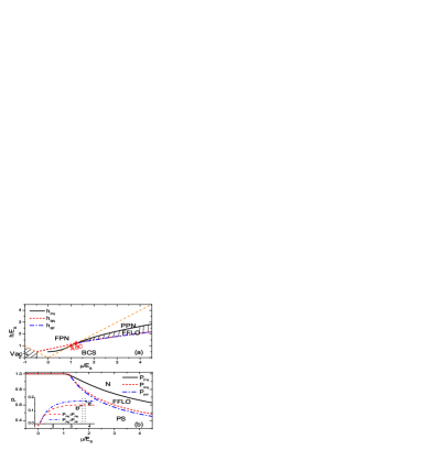
Figure 1: (color online) Phase diagrams of a 2D Fermi gas. (a)$h-\mu$ diagram constructed by vacuum, BCS, FFLO, partially polarized normal (PPN) and fully polarized normal (FPN) states. The boundary $h_{BF}$ is just slightly below $h_{BN}$. Red cross points $(\mu/E_{B},h/E_{B})$ from left to right: $A(1,1)$, $B(\frac{\sqrt{2}+1}{2},\frac{\sqrt{2}+1}{2})$ and $C(\frac{5}{4},\sqrt{\frac{3}{2}})$ correspond to $h_{FN}=\mu$, $h_{BN}=\mu$ and $h_{FN}=h_{BN}$ respectively. Orange dashed line is for $h=|\mu|$. (b)$P-\mu$ diagram constructed by phase separation (PS), FFLO and normal (N) states. Inset shows two $\Delta P$ plots $\Delta P_{1}=P_{FN}-P_{PN}$ and $\Delta P_{2}=P_{FN}-P_{PF}$, with each peak $(\mu/E_{B},\Delta P_{max})$ locating respectively at $D(3.605,0.146)$ and $E(3.750,0.177)$.

The phase diagrams for a 2D Fermi gas are shown in Fig. 1, and here three points are emphasized in order. First, numerical simulations show that the FFLO-N boundary $h_{FN}$, which is the maximum value of $h_{c}$ at certain non-zero $q$, shows up immediately when $\mu>0$, but is less than the BCS-N boundary $h_{BN}$ until $\mu$ up to $\frac{5}{4}E_{B}$ at point C [shown in Fig. 1(a)]. Only beyond C, FFLO can exist as a candidate of ground state. Second, Fig. 1(b) shows that the maximum polarization window for FFLO state to exist as ground state is less than $20\%$, even when taking into account the small distinction between $h_{BF}$ and $h_{BN}$. Third, throughout the range of $\mu$, there is no stable magnetized superfluid ($SF_{M}$) phase found as that in the strong coupling limit in 3D free space. One powerful piece of evidence is that the Sarma-N boundary ($h_{SN}$) can never exceed the lowest BCS excitation energy ($E_{min}$),

$$h_{SN} = \left\{\begin{array}[]{l}E_{B}/2,\ \ \ \ \ \ |\mu|\leq E_{B}/2\\ \sqrt{\mu E_{B}/2},\ \ \mu>E_{B}/2\end{array}\right.$$ (18)

$$E_{min} = \left\{\begin{array}[]{l}\mu+E_{B},\ \ \ \ -E_{B}/2<\mu\leq 0\\ \sqrt{E_{B}(2\mu+E_{B})},\ \ \ \ \ \ \ \mu>0\end{array}\right.$$ (21)

implying the exclusion of $SF_{M}$ from the ground-state solutions. Here $h_{SN}$ is obtained by solving the gap equations at zero gap amplitudes. We also use this criterion to judge the existence of $SF_{M}$ in the following calculations for optical lattices.

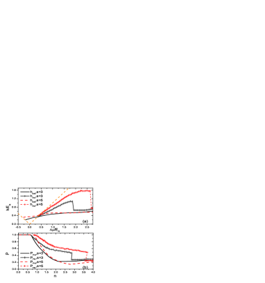
Figure 2: (Color online) Phase diagrams of a 2D Fermi gas when applying optical lattices along an arbitrary direction with different depths $s=3,5$. The gas is in the weak interacting regime with the two-body binding energy $E_{B}=0.2E_{R}$. (a)$h-\Delta\mu$ diagram with $\Delta\mu$ calculated from the bottom of the lowest band. Orange dashed line is for $h=|\Delta\mu|$ defining the threshold for a fully polarized normal state. BCS, FFLO and normal states are separated by the corresponding boundaries as labeled in the legend. FFLO exists as the ground state when $h_{BN}<h<h_{FN}$. (b)$P-n$ diagram. From the bottom to top are phase seperation, FFLO and normal state in turn. At a certain density, $P_{FN}$ suddenly drops to a lower value corresponding to the same behavior of $h_{FN}$ in (a).

When applying an optical lattice along one direction the phase diagrams are dramatically changed as shown in Fig. 2. First we study the low density limit. It is observed that the minimum density for FFLO to exist, $n_{min}$, moves to the right (becomes large) as lattice potential $s$ increases. We argue that this indicates a much more enhanced coupling of atoms moving in deeper lattices. Actually this critical point ($n_{min}$) is an analog of point C in Fig. 1(a) for free 2D system, in which $n_{min}$ monotonously increases with $\mu_{C}(=5E_{B}/4)$ and also $E_{B}$. Optical lattices applied here drive the system to a strongly interacting regime characterized by the enhanced effective binding energies and thus increase $n_{min}$. Moreover, in this dilute limit the maximum of critical chemical potential differences $h_{c}(q)$ is always at $q=0$ (see Fig. 3(a)), indicating no FFLO but only an unstable Sarma state ($h_{SN}<E_{min}$).

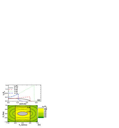
Figure 3: (Color online) (a)Critical chemical potential differences $(h_{c})$ as a function of total pairing momenta $(q)$ at several averaged chemical potentials ($\Delta\mu$) with lattice potential $s=5$. (b)Fermi surface contour in momentum space. The optical lattice is applied along x direction. The inner and outer red dashed lines respectively represent the Fermi surfaces at the top of the lowest band (labeled by 0.264) and slightly beyond the bottom of a higher band (2.73). The outer line also corresponds to the dashed-dotted curve in (a).

Second we observe that as the density $n$ or $\mu$ increases, the FFLO-N boundary $h_{FN}$ initially goes up but then suddenly drops at certain position, the reason for which is illustrated in Fig. 3. As $n$ increases, $h_{FN}$ with nonzero pairing momentum $q$ starts to exceed $h_{BN}$ which stabilizes FFLO states. Meanwhile, the shape of Fermi surface distorts from an ellipse to two disconnected lines, implying a crossover from 2D to a quasi-1D geometry and correspondingly $h_{FN}$ has a rapid increase during the crossover. When $n$ increases further, the shape of Fermi surface changes again when atoms begin to fill a higher lattice band. However, this occupation of a higher band exposes a destructive effect on FFLO pairing along the free direction. For example Fig. 3(a) shows that the maximum value of $h_{c}$ for $\Delta\mu/E_{R}=2.73$ is much less than that for $2.43$, leading to a sudden drop of $h_{FN}$ as well as $P_{FN}$ in Fig. 2. Moreover, it is noticed that the discontinuity of $h_{FN}$ in this sensitive region produces double values of $P_{FN}$ at a definite density $n$ as a side effect, in which case the larger one should be chosen as the real critical polarization for FFLO. Finally it is shown by Fig. 2(b) that at intermediate $n$ the PS-N boundary $P_{PN}$ is suppressed by increasing $s$, in contrast to $P_{FN}$. We attribute this to the discontinuous lattice spectrum that reduces the Hilbert space for pairing and therefore disfavors the BCS superfluidity.

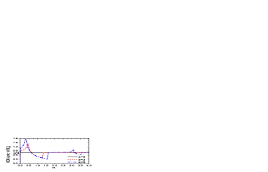
Figure 4: (Color online) Density of state (DOS) scaled by $1/(a^{2}E_{R}$) at the Fermi surface versus particle densities $n=Na^{2}/S$. Optical lattices are applied along an arbitrary direction in 2D space with different depths $s=0,3,5$. In free space ($s=0$), DOS is a constant ($\pi/4$).

Finally we comment that these effects of optical lattices at low and intermediate densities can be well understood from the point of view of density of state (DOS), see also Fig. 4. The variations of DOS bring two opposite effects to the BCS superfluidity (SF) and FFLO. At low densities ($n$), DOS is enhanced by the optical lattices applied and therefore favors SF but disfavors FFLO as a result of the strong effective couplings; at intermediate $n$, DOS decreases with $n$ which approximately satisfies $DOS\sim 1/n$ indicating the evolution to 1D geometry, so this time FFLO is favored while SF is suppressed. When $n$ further increases, DOS becomes stable at the same level as in 2D free gas when atoms start to fill a higher lattice band. After this point the quasi-1D geometry fades away and FFLO is no longer favored.

III.2 Quasi-1D and quasi-2D geometries in a 3D space

The quasi-1D geometry in 3D space is formed by applying optical lattices along two orthogonal directions. The theoretical model has been outlined in Sec. II, and here we present the phase diagrams in Fig. 5.

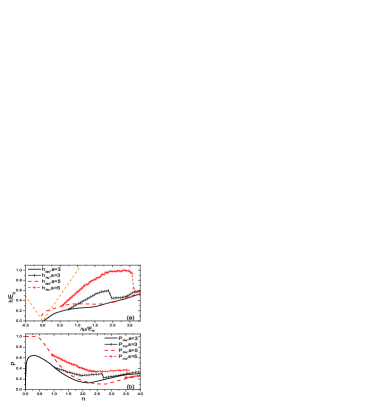
Figure 5: (color online) Phase diagrams of a 3D Fermi gas when applying optical lattices along two orthogonal directions with different depths $s=3,5$. The s-wave scattering length is fixed to be $a_{s}=-a/3$. (a)$h-\Delta\mu$ diagram. Orange dashed line is for $h=|\Delta\mu|$. (b)$P-n$ diagram. Each boundary separates corresponding phases in the same way as in Fig. 2.

At a given low density ($n$), the maximum polarization for phase separation ($P_{PN}$) increases from a small value to unity with lattice potential $s$, in contrast to quasi-1D geometry in 2D space; however it does reveal the same fact that optical lattices enhance the effective coupling. Moreover in this region, $h_{FN}<h_{BN}$ so actually FFLO will not serve as a candidate for ground states. As $n$ continues to increase, the system undergoes a crossover to quasi-1D geometry, and $h_{FN}$ gradually goes up. Compared with a negligible FFLO polarization window for the 3D free Fermi gas, the optical lattice with $s=5$ can broaden the window from as large as $25\%$ at the optimum density $n\simeq 2.5$. When $n$ or $\mu$ is large enough to touch a higher lattice band, $h_{FN}$ and $P_{FN}$ again suffer from a drop behavior as introduced in the previous section.

Next we turn to quasi-2D geometry in 3D space which could be generated by an axial optical lattice. We do not present the phase diagrams here but give a brief introduction. Compared with quasi-1D geometry the available FFLO window in this case is much less robust, for instance less than $10\%$ with lattice potential $s=5$. Moreover there is no obvious sudden drop of $h_{FN}$ or $P_{FN}$. This might be ascribed to two tunable parameters ($|q|$ and $\theta$) in this case for FFLO pairing momentum vector $(q_{x},q_{y})=|q|(\cos\theta,\sin\theta)$, which make the pairing relatively flexible and easily adaptive to external variations.

IV Phase profile under external harmonic confinements

In this section, we study the effect of asymmetric lattices to the phase profile of imbalanced fermions in a harmonic trap using local density approximation (LDA). In LDA, locally the gas is considered to have the same properties as a bulk gas, which depend on the local averaged chemical potentials $\mu(\mathbf{r})=(\mu_{0\uparrow}+\mu_{0\downarrow})/2-V(\mathbf{r})$ and position-independent difference $h=(\mu_{0\uparrow}-\mu_{0\downarrow})/2$. $\mu_{0\sigma}(\sigma=\uparrow,\downarrow)$ is the chemical potential of spin-$\sigma$ atoms at the trap center, and can be self-consistently determined by the total particle numbers $N_{\sigma}$, s-wave interactions and lattice potentials.

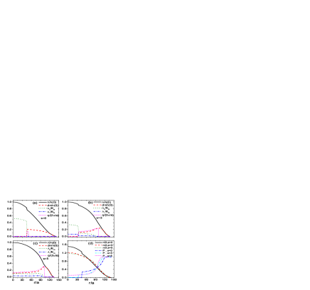
Figure 6: (color online). (a,b,c) Spatial distributions of the normalized total density ($n/n(0)$), density difference ($dn/n(0)$), gap amplitudes ($\Delta_{0},\Delta_{1}$), FFLO pairing momentum $q_{z}$ for a density-imbalanced two-species ${}^{6}Li$ Fermi gas. $n(0)=N(0)a^{3}/V$ is the dimensionless total density at the trap center. The optical lattices $s=0(a),3(b),5(c)$ are applied along $x$ and $y$ directions with lattice constant $a=532nm$. An isotropic harmonic trap is also applied with trapping frequency $f=200Hz$. The s-wave scattering length is fixed to be $a_{s}=-a/3$. Other parameters are chosen so that these three plots (a,b,c) have nearly identical particle numbers: $s,N/2,P,h/E_{R},n(0)=0,4.3(10^{6}),0.42,0.31,3.03(a)$; $3,4.35(10^{6}),0.42,0.32,2.44(b)$; $5,4.45(10^{6}),0.43,0.34,2.35(c)$. (d) Spatial distributions of the averaged total density ($n/2$) and polarization ($P$) corresponding to (a-c).

In Fig. 6 we give three typical phase profiles under an external isotropic harmonic trap. The optical lattices are applied in two orthogonal directions and form an array of 1D tubes in 2D lattice sites. Using LDA, we solve the ground state at each position by minimizing the thermodynamic potential $\Omega(\Delta_{0},\Delta_{1},q_{z})$ in terms of its three parameters. Meanwhile $\mu_{0\uparrow}$ and $\mu_{0\downarrow}$ are adjusted such that the particle numbers are almost identical for different $s$. Therefore Fig. 6 actually shows how the phase profile of an imbalanced Fermi gas in a harmonic trap evolves when switching on the optical lattices, especially for the FFLO state. Without lattices ($s=0$), the profile is mostly constructed by BCS and normal state, with negligible FFLO window in between. While increasing $s$, the window is gradually broadened. For $s=3$, the spatial range of FFLO has extended to be nearly as the same as that of BCS and normal state. During this period, particles move from center and edge to the middle region, causing both $n(0)$ (density in the trap center) and $R_{TF}$ (Thomas-Fermi radius) to decrease correspondingly. By increasing $s$ further, FFLO would gradually spread to the trap center and take over BCS state, until finally only FFLO and normal state are left in the trap, see Fig. 6(c) for $s=5$. Moreover, notice that the discontinuities of densities $n_{\sigma}$, gap amplitudes $\Delta_{0},\Delta_{1}$ at the BCS-FFLO boundary imply a first-order phase transition, while the continuities at FFLO-N boundary imply a continuous transition.

Finally two statements about FFLO are given as follows. First, FFLO should be observed far away from the trap edge due to the atomic dilution and strong effective interactions there; second, its spatial range is enlarged by the increasing geometric asymmetry.

V summary

In conclusion, we have studied the phase diagrams of imbalanced two-species fermions in asymmetric optical lattices. We found that the optical lattices applied expose two opposite effects on the BCS and FFLO states, depending on the atomic densities. One is to enhance the effective interaction at low densities which favors BCS but destroys FFLO; the other is to induce the crossover to lower dimension at intermediate fillings which favors FFLO, but destroys BCS due to the discontinuity of lattice energy spectrum. Among all the asymmetric geometries, we find that the quasi-1D system is the most favorable one for observing the FFLO state. Finally by using LDA, we present several typical phase profiles in a harmonic trap with substantially different FFLO proportions, which are merely tuned by the potential depths of applied asymmetric optical lattices. These lattice effects still need to be further explored in cold-atom experiments.

We are grateful to Wei Zhang for many stimulating discussions. This work was financially supported by the National Science Foundating of China, Chinese Academy of Sciences (CAS) and the 973-project of Ministry of Science and Technology (MOST), China.

References

- (1) M. W. Zwierlein, A. Schirotzek, C. H. Schunck, W. Ketterle, Science 311, 492 (2006).
- (2) G. B. Partridge, W. Li, R. I. Kamar, Y. Liao, R. G. Hulet, Science 311, 503 (2006).
- (3) M. W. Zwierlein, C. H. Schunck, A. Schirotzek, W. Ketterle, Nature 442, 54 (2006).
- (4) Y. Shin, C. H. Schunck, A. Schirotzek, W. Ketterle, Nature 451, 689 (2008).
- (5) P. F. Bedaque, H. Caldas, G. Rupak, Phys. Rev. Lett. 91, 247002 (2003).
- (6) D. E. Sheehy and L. Radzihovsky, Phys. Rev. Lett. 96, 060401 (2006).
- (7) H. Hu and X. J. Liu, Phys. Rev. A. 73, 051603(R) (2006).
- (8) M. M. Parish, F. M. Marchetti, A. Lamacraft and B. D. Simons, Nature Physics 3, 124 (2007).
- (9) W. Zhang and L. M. Duan, Phys. Rev. A. 76, 042710 (2007).
- (10) G. Sarma, J. Phys. Chem. Solids 24, 1029 (1963).
- (11) W. V. Liu and F. Wilczek, Phys. Rev. Lett. 90, 047002 (2003);
- (12) P. Fulde, R. A. Ferrell, Phys. Rev. 135, A550 (1964); A. I. Larkin, Y. N. Ovchinnikov, Sov. Phys. JETP 20, 762 (1965).
- (13) N. Yoshida and S.-K. Yip, Phys. Rev. A 75, 063601 (2007);
- (14) H. Hu, X. J. Liu and P. D. Drummond, Phys. Rev. Lett. 98, 070403 (2007); X. J. Liu, H. Hu and P. D. Drummond, Phys. Rev. A. 76, 043605 (2007).
- (15) G. Orso, Phys. Rev. Lett. 98, 070402 (2007).
- (16) G. J. Conduit, P. H. Conlon and B. D. Simons, Phys. Rev. A. 77, 053617 (2008).
- (17) T. K. Koponen, T. Paananen, J.-P. Martikainen, P. Törmä, Phys. Rev. Lett. 99, 120403 (2007); T. K. Koponen, T. Paananen, J.-P. Martikainen, M.R. Bakhtiari, P. Törmä, New J. Phys. 10, 045014 (2008).
- (18) M. M. Parish, S. K. Baur, E. J. Mueller and D. A. Huse, Phys. Rev. Lett. 99, 250403 (2007).
- (19) A. E. Feiguin and F. Heidrich-Meisner, Phys. Rev. Lett. 102, 076403 (2009).
- (20) X.-L. Cui and Y.-P. Wang, Phys. Rev. B 79, 180509(R)(2009).
- (21) E. G. Moon, P. Nikoli, and S. Sachdev, Phys. Rev. Lett. 99, 230403 (2007).
- (22) C. Comte and P. Nozières, J. Phys. (Paris) 43, 1069 (1982).
- (23) P. Nozières and S. Schmitt-Rink, J. Low Temp. Phys. 59, 195 (1985).
- (24) J.-P. Martikainen, E. Lundh and T. Paananen, Phys. Rev. A. 78, 023607 (2008).
- (25) D. S. Petrov and G. V. Shlyapnikov, Phys. Rev. A. 64, 012706 (2001).
- (26) L.-Y. He and P.-F. Zhang, Phys. Rev. A. 78, 033613 (2008).
- (27) H. Shimahara, Phys. Rev. B 50, 12760 (1994).
- (28) R. Combescot and C. Mora, Eur. Phys. J. B 464, 189 (2005).