Femtosecond laser pulse shaping for enhanced ionization

Abstract

We demonstrate how the shape of femtosecond laser pulses can be tailored in order to obtain maximal ionization of atoms or molecules. For that purpose, we have overlayed a direct-optimization scheme on top of a fully unconstrained computation of the three-dimensional time-dependent Schrödinger equation. The procedure looks for pulses that maintain the same total length and integrated intensity or fluence as a given pulse that serves as an initial guess. It allows, however, for changes in frequencies – within a certain, predefined range – and overall shape, leading to enhanced ionization. We illustrate the scheme by calculating ionization yields for the H${}_{2}^{+}$ molecule when irradiated with short ($\approx 5$ fs), high-intensity laser pulses.

1 Introduction

When atoms or molecules are irradiated with laser fields that are intense enough to induce nonlinear effects, a wealth of fascinating phenomena may be observed [1]. This applies even to deceitfully “uninteresting” systems such as the simplest molecule, H${}_{2}^{+}$ [2]: above-threshold or tunneling ionization [3], bond softening [4], bond hardening (light induced bound states or vibrational trapping) [5], charge resonance enhanced ionization [6, 7], above threshold dissociation [8], high harmonic generation [9], etc.

This very same complexity in the molecular reaction, however, is what permits to envision the possibility of controlling molecules with short (femtosecond time scale) and intense (10${}^{11}-10^{15}$ W/cm²) laser pulses [10]. The short durations allow for coherent control: the systems evolve uncoupled to the environment, and can be steered towards the desired outcomes without relying in the more traditional control parameters, i.e., average, thermodynamic functions such as the temperature. The high intensities trigger the strongly nonlinear, even non-perturbative, response of the systems. An essential ingredient to realize the molecular control is the capability of shaping the laser pulses – a technological area that has witnessed spectacular advances in the recent years [11].

Yet this complexity implies the need for challenging theoretical models. Not surprisingly, ionization is the first and most studied process, mainly because it could already be studied for atoms [12], and because in this intensity regime it almost always occurs, be it accompanied or not by other phenomena. Even in the absence of influence from nuclear dynamics, the ionization of molecules is significantly more complex than that of atoms, due to the electron emission from different atomic centers [13, 14]. Two rather successful models for molecular ionization that have recently been suggested are the so-called molecular-orbital strong-field approximation [13] and the molecular extension of the Ammosov-Delone-Kraine (ADK) approximation [15]. However, these approaches are insufficient as general tools [16].

A common feature of the approaches mentioned above is the use of the single-active-electron (SAE) approximation. One-electron molecular systems such as the hydrogen molecular ion H${}_{2}^{+}$ are therefore perfect candidates to isolate the error introduced by the SAE approximation from further simplifications. Electron correlation originates difficult and interesting phenomena such as non-sequential ionization [17].

In order to properly investigate the interaction of short and intense laser fields with molecules, one needs to perform explicitly time-dependent calculations, even if it might imply a heavy computational burden. Calculations of this kind, that propagate the time-dependent Schrödinger equation (TDSE), have been presented for H${}_{2}^{+}$ in the past, for example with the purpose of understanding the presence of maxima in the ionization yield for particular internuclear separations [18], or in order to disentangle the relationship between ionization and dissociation [19, 7]. Recently, Selstø et al. [20] and Kjeldsen et al. [21] have reported calculations on the orientation dependence of the ionization yield – lifting the commonly used assumption of a molecular axis parallel to the light polarization.

In this work we take a further step, and focus on the possibility of theoretically designing, via fixed-nuclei three-dimensional (3D) TDSE calculations, laser pulses able to control (in particular, significantly enhance) the ionization yields, taking H${}_{2}^{+}$ as an example system. Some recent experimental breakthroughs on this area have triggered our interest. For example, Suzuki et al. [22] demonstrated the control of the multiphoton ionization channels of I₂ molecules by making use of a pulse shaping system capable of varying in time the polarization directions. Simultaneously, Brixner et al. [23] have made use of a similar polarization-shaping system to enhance ionization yields of diatomic molecules (K₂). Our focus is, however, on linearly polarized ultrashort pulses ($\approx$ 5 fs), so rapid that the nuclear movement does not play a role during the pulse action – in contrast to the studies in which the ionization is studied as the internuclear distance changes, leading to possible resonances.

2 Methodology

The optimization problem could be formulated in the language of quantum optimal-control theory (QOCT) [24]. It consists of a set of equations – along with various suitable, iterative algorithms that solve them – whose solution provides an optimized control field that typically maximizes a target operator $\hat{O}$. In order to enhance ionization, one would just define ${\hat{O}}$ as the projection onto unbound states, or, alternatively, the identity minus the projection onto the bound states:

$$\hat{O}=\hat{1}-\sum^{\rm bound}_{i}|\varphi_{i}\rangle\langle\varphi_{i}|\,.$$ (1)

However, we have experienced numerical difficulties when attempting to solve the QOCT equations for this particular operator: The forward-backward propagations that must be performed in order to solve the QOCT equations proved to be, for our particular implementation, numerically unfeasible when using the operator given in Eq. (1) to define the target. This was due to the appearance of fields with unrealistically high frequencies and/or amplitudes. We believe that the reason lies in the fact that the backward propagation must be performed after acting with the operator $\hat{O}$ on the previously propagated wave function. This eliminates the smooth, numerically friendly part of the wave function, enhancing, on the contrary, the high frequency components. This procedure is repeated at each iteration, eventually making the propagation impossible. We do not claim, however, that any other numerical implementation will not be able to successfully cope with this problem.

Therefore, we have employed and present here, a direct optimization scheme, which is in fact much closer in spirit to the techniques utilized by the experimentalists [25]. In this scheme, we construct a merit function by considering the expectation value of the operator defined in Eq. (1) at the end of the propagation:

$$F(x)=\langle\Psi_{x}(T)|\hat{O}|\Psi_{x}(T)\rangle\,,$$ (2)

where $x$ is the set of parameters that define the laser pulse, and $|\Psi_{x}(T)\rangle$ is the wave function that results from performing the propagation with the laser determined by $x$, at the final time $T$. Of course, the sum over the bound states has to be truncated; for the calculations presented below, we find it sufficient to include the lowest ten states. The merit function is calculated by performing consecutive TDSE propagations: The resulting function values are fed into a recently developed derivative-free algorithm called NEWUOA [26]. This algorithm seeks the maximum of any merit function $F(x)$ depending on $N$ variables $x$, and does not necessitate the gradient $\nabla F$. It is very effective for $N$ larger than ten and smaller than a few hundred, which is the case considered here. In all our runs, we necessitated around two hundred iterations to converge the ionization yields to within 1%.

The system and the TDSE propagations are modeled in our homegrown octopus code [27]. We represent the wave functions on a real-space rectangular regular grid, and fix the nuclear position at their equilibrium distance. The small length of the pulses used here justifies this simplification. We perform calculations setting the polarization direction both parallel to the molecular axis and perpendicular to it. The size of the simulation box is selected large enough to ensure that very little of the electronic density has reached the grid boundaries at the end of the laser pulse. Nevertheless, we add absorbing boundaries to remove this charge; if the propagation is pursued after the pulse, part of the density will “abandon” the simulation box; the remaining integrated density should approach (as it does) one minus the ionization probability calculated as the expectation value of Eq. (1).

The laser pulse is taken in the dipolar approximation, and represented in the length gauge. The temporal shape of the pulse is given by a function $f(t)$, which we expand in a Fourier series:

$$f(t)=f_{0}+\sum_{n=1}^{N}\left[f_{n}\sqrt{\frac{2}{T}}\cos(\omega_{n}t)+g_{n}\sqrt{\frac{2}{T}}\sin(\omega_{n}t)\right]\,,$$ (3)

with $\omega_{n}=2\pi n/T$. In order to ensure a physically meaningful laser pulse [28], we must have $\int_{0}^{T}{\rm d}tf(t)=0$, which implies $f_{0}=0$. Moreover, we must have $f(0)=f(T)=0$, where $T$ is the total propagation time. This poses the following constraint:

$$\sum_{n=1}^{N}f_{n}=0\,.$$ (4)

The sum over frequencies is truncated according to physical considerations: Any pulse shaper must have a predefined range of frequencies it can work with. The feasibility of the numerical scheme depends on the possibility of truncating the previous expression at a reasonably low number. In the cases considered here, due to the short duration of the pulses, we obtain no more than around 20 degrees of freedom by setting the maximum frequency to one Hartree.

Evidently, by increasing the intensity of a pulse one can enhance the ionization yield. Our wish is to improve this yield by changing the pulse shape, and not simply by lasing with larger intensity. Therefore, to ensure the fairness in the optimization search, we constrain the search to laser pulses whose time-integrated intensity (fluence) is predefined to some value $F_{0}$:

$$F_{0}=\int_{0}^{T}\!\!\!\!f^{2}(t)\,{\rm d}t=\sum_{n=1}^{N}(f_{n}^{2}+g_{n}^{2})\,.$$ (5)

The search space $\{f_{n},g_{n}\}$ is thus constrained to the hyper-sphere defined by the previous equation. But we must add the condition given by Eq. (4), which further restricts the search space to a hyper-ellipsoid. By performing the appropriate unitary transformation, this can be brought again into a hypersphere:

$$F_{0}=\sum_{n=1}^{2N-1}\xi_{n}^{2}\,.$$ (6)

This equal-fluence condition can be guaranteed if we perform a new transformation to hyperspherical coordinates:

$$\xi_{1} = F_{0}^{1/2}\cos(\theta_{1})\,,$$

$$\xi_{2} = F_{0}^{1/2}\sin(\theta_{1})\cos(\theta_{2})\,,$$

$$\dots = \dots$$

$$\xi_{2N-2} = F_{0}^{1/2}\sin(\theta_{1})\dots\sin(\theta_{2N-3})\cos(\theta_{2N-2})\,,$$

$$\xi_{2N-1} = F_{0}^{1/2}\sin(\theta_{1})\dots\sin(\theta_{2N-3})\sin(\theta_{2N-2})\,.$$ (7)

The set of angles $\{\theta_{j}\}_{j=1}^{2N-2}$ constitute the $2N-2$ variables that define the search space for the optimization algorithm.

3 Results

The initial laser field before the optimization is a linearly polarized eight-cycle pulse having a sinusoidal envelope, fixed peak intensity, and wavelength of $\lambda=400$ nm – a typical value for frequency-doubled Titanium-sapphire lasers. Correspondingly, the initial frequency is $\omega_{0}=0.114$ Ha, and the pulse length is $5.3$ fs. The maximum allowed frequency of the optimized pulse is set to $\omega_{\rm max}=2\,\omega_{0}$. The pulse polarization is fixed to be parallel or perpendicular to the molecular axis. During the QOCT procedure, the polarization and the fluence $F_{0}$ are kept fixed, but the peak intensity may change from the initial value, which is selected in the range $I=0.5,0.75,\ldots,2\times 10^{15}$ W/cm².

Figure 1

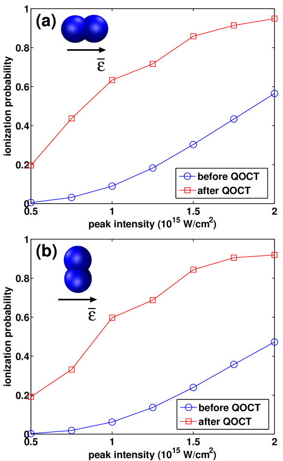
Figure 1: (color online). Ionization probability for the initial pulse (circles) and for the optimized pulse (squares) as a function of the peak intensity of the initial pulse. The polarization of the pulse is (a) parallel and (b) perpendicular to the molecular axis.

shows the ionization probabilities as a function of the peak intensity (of the initial guess pulse) for the initial and optimized pulses polarized parallel (a) and perpendicular (b) to the molecular axis, respectively. Overall, the pulse optimization leads to a significant increase in the ionization. As expected, the ionization yield is slightly larger for pulses polarized parallel to the molecular axis.

To get more insight into the optimized ionization process, we plot in Fig. 2

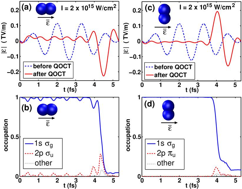
Figure 2: (color online). (a) Initial and optimized pulses (parallel polarization) and (b) the occupation of selected single-electron states in the optimized ionization process, when $I=2\times 10^{15}$ W/cm². (c-d) Same as (a-b) but for perpendicular polarization.

the initial and optimal laser pulses and the occupations of some single-electron states during the pulse interaction. The peak intensity of the initial pulse is $I=2\times 10^{15}$ W/cm². Optimized pulses of both parallel (a) and perpendicular (c) polarization have large peaks near the end of the pulse. According to the corresponding occupations shown in Figs. 2(b) and (d), these amplitude peaks account for almost all of the ionization: During the peaks the ground-state occupations rapidly collapse. The 2p $\sigma_{\rm u}$ (2p $\pi_{\rm u}$) excited state contributes to the process to a small extent in the parallel (perpendicular) case, whereas the other states are involved by a nearly negligible fraction; overall, no excited bound states contribute significantly. Hence, within the constraints set here for the laser pulse, the optimal ionization of H${}_{2}^{+}$ is a direct process obtained by focusing most of the available pulse energy in a very short time frame – though keeping the integrated total field at zero in accordance with Maxwell’s equations (see Ref. [28]). The electron densities during the ionization process are visualized in Fig. 3

Figure 3: (color online). (a-f) Snapshots of the electron densities in the optimized ionization process when the pulse polarization is parallel to the molecular axis and the intensity is $I=2\times 10^{15}$ W/cm². The black dots mark the positions of the nuclei. The time-steps between snaphots are all equal. (g-l) The same for a pulse polarized perpendicular to the molecular axis.

for both parallel (a) and perpendicular (b) polarizations.

The previous optimizations have produced rather “uninteresting” solutions. It is a well known fact that in a short intense laser pulse, most of the ionization occurs during the peaks in the electric field. Therefore, the optimizations have just attempted to create short, intense bursts of light. This fact can be understood if we consider the process happening in the quasi-static, tunneling regime, in which the total ionization can be approximated by considering at each moment in time the static ionization rate that corresponds to the electric amplitude. This ionization rate is nonlinear, and it is much larger at the electric field peaks, which therefore cause most of the ionization. Note, however, that the cases discussed above lie in an intermediate regime between the tunneling and the multi-photon regime – the Keldysh parameter, $\gamma$, is of the order of one [The Keldysh parameter $\gamma$ is defined as $\sqrt{|E_{I}|/2U_{p}}$, where $E_{I}$ is the ionization potential of the system, and $U_{p}$ is the pondemorotive energy, given in atomics units by $(E_{0}/2\omega)^{2}$, $E_{0}$ being the peak intensity of the electric field, and $\omega$ the pulse frequency. Since our optimized lasers do not have a single frequency – not even necessarily a dominant one, we can only speak of approximate Keldysh parameters.]

Alternatively, one can explain the simplicity of the pulses considering that the maximum allowed frequency, $2\,\omega_{0}=0.228$ Ha, is smaller than any resonance transition energy from the ground state. As a consequence, the system does not significantly populate these states, and the only ionizing channel is direct transition to the continuum.

The picture changes significantly, however, if we allow for a larger cutoff frequency. First, this increases the value of the Keldysh parameter associated with the process, which may change the regime from a more quasistatic to a more of a multi-photon-like character. Secondly, the excited bound states are now accessible for single-photon transitions. For example, Fig. 4 displays results obtained for $4\,\omega_{0}$. The intensity is here set to $0.5\times 10^{15}$ W/cm². Doubling the cutoff frequency of the search space has a significant effect in the total ionization yield: Now we obtain 0.99 for the ionization probability, whereas in the first optimization the yield was 0.20 (see Fig. 1, top panel, first point in the series). Note that the initial yield before any optimization was only 0.005.

Moreover, the manner in which the ionization occurs with a larger cutoff frequency is qualitatively very different. Figure 4

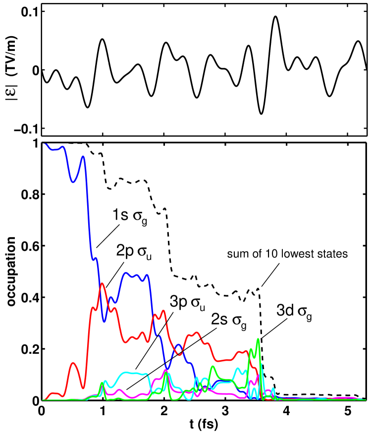
Figure 4: (color online). Upper panel: Optimized laser pulse for the ionization when the cutoff frequency is $4\,\omega_{0}$ (see text) and the intensity is fixed to $0.5\times 10^{15}$ W/cm². Lower panel: Occupation of a few lowest states during the pulse interaction.

displays the evolution of the occupation of some of the bound states. The first excited state ($2{\rm p}\,\sigma_{\rm u}$) plays a significant role, which can be understood because the transition energy from the ground state is now accessible in the field search space. In addition, a couple of other lowest states contribute in the ionization process in an ascending order as a function of time. It should be noted, however, that only the $\sigma$ orbitals, where the nodes are perpendicular to the polarization axis, participate in the transitions, and $\pi$ orbitals, for example, are not allowed due to a different symmetry. As a consequence of the involvement of several states in the ionization process, the structure of the optimized laser pulse shown in the upper panel of Fig. 4 is much more complicated than the single-burst fields obtained in the previous calculations.

4 Conclusions

In conclusion, we have shown with three-dimensional time-propagations of the time-dependent Schrödinger equation how the precise temporal shape of a short intense laser pulse may affect significantly the total ionization yield of H${}_{2}^{+}$ at fixed internuclear separations. Moreover, we have employed a gradient-free optimization technique to find the laser pulse that enhances ionization. This optimization can be constrained in different ways, accounting for the limitations of physical sources – not all frequencies and intensities are available, and not all possible shapes can be constructed with the state-of-the-art pulse shapers (although the technology improves at a phenomenal rate). The results will differ depending on these constraints: The optimized laser pulse may be the single burst of electric field that one would expect by considering a process in the tunnelling regime, or a field with a more complicated structure that drives the system through intermediate states – the ionization can be enhanced by resonant transitions. Whereas in the former case it would be easy to design intuitively pulses that maximize the ionization, in the latter an optimization algorithm such as the one presented in this work is necessary.

- [1] \NameBrabec T. Krausz F. \REVIEWRev. Mod. Phys. 722000545; \NamePosthumus J. H. \REVIEWRep. Prog. Phys672004623; \NameScrinzi A., Ivanov M. Y., Kienberger R. Villeneuve D. M. \REVIEWJ. Phys. B: At. Mol. Phys.392006R1.
- [2] \NameGiusti-Suzor A., Mies F. H., DiMauro L. F., Charron E. Yang B. \REVIEWJ. Phys. B: At. Mol. Opt. Phys.281995309.
- [3] \NameGibson G. N., Li M., Guo C. J. Neira \REVIEWPhys. Rev. Lett.7919972022; \NameVafaee M. H. Sabzyan \REVIEWJ. Phys. B: At. Mol. Opt. Phys.3720044143; \NameBen-Itzhak I., Wang P. Q., Xia J. F., Sayler A. M., Smith M. A., Carnes K. D. B. D. Esry \REVIEWPhys. Rev. Lett.952005073002; \NamePavičić D., Kiess A., Hänsch T. W., Figger H. \REVIEWPhys. Rev. Lett942005163002.
- [4] \NameBucksbaum P. H., Zavriyev A., Muller H. G. Schumacher D. W \REVIEWPhys. Rev. Lett6419901883.
- [5] \NameGiusti-Suzor A. Mies F. H. \REVIEWPhys. Rev. Lett.6819923869; \NameFrasinski L. J., Posthumus J. H., Plumridge J., Codling K., Taday P. F., Langley A. J. \REVIEWPhys. Rev. Lett.8319993625.
- [6] \NameZuo T., Chelkowski S. Bandrauk A. D. \REVIEWPhys. Rev. A4819933837; \NameZuo T. Bandrauk A. D. \REVIEWPhys. Rev. A521995R2511.
- [7] \NameChelkowski S., Conjusteau A., Zuo T. Bandrauk A. \REVIEWPhys. Rev. A5419963235.
- [8] \NameGiusti-Suzor A., He X., Atabek O. Mies F. H. \REVIEWPhys. Rev. Lett.641990515.
- [9] \NamePlummer M. McCann J. F. \REVIEWJ. Phys. B: At. Mol. Opt. Phys.281995L119.
- [10] \NameShapiro M. Brumer P. \BookPrinciples of the Quantum Control of Molecular Processes \PublWiley, New York \Year2003; \NameRice S. A. Zhao M. \BookOptical Control of Molecular Dynamics \PublJohn Wiley & Sons, New York \Year2000; \BookAnalysis and Control of Ultrafast Photoinduced Reactions \EditorKühn O. Wöste L. \PublSpringer, Heidelberg \Year2007.
- [11] \NameWeiner A. M. \REVIEWRev. Sci. Instrum7120001929.
- [12] \NameProtopapas M., Keitel C. H. Knight P. L. \REVIEWRep. Prog. Phys.601997389.
- [13] \NameMuth-Böhm J., Becker A. Faisal F. H. M. \REVIEWPhys. Rev. Lett.8520002280.
- [14] \NameLitvinyuk V., Lee K. F., Dooley P. W., Rayner D. M., Villeneuve D. M. Corkum P. B. \REVIEWPhys. Rev. Lett.902003233003; \NameKjeldsen T. K., Bisgaard C. Z., Madsen L. B. Stapelfeldt H. \REVIEWPhys. Rev. A712005013418.
- [15] \NameTong X. M., Zhao Z. X. Lin C. D. \REVIEWPhys. Rev. A662002033402.
- [16] For a recent discussion see, for example: \NameAwasthi M., Vanne Y. V., Saenz A., Castro A. Decleva P. \REVIEWPhys. Rev. A772008063403.
- [17] \NameWalker B. \REVIEWPhys. Rev. Lett.7319941227; \NameFaisal F. H. M. Becker A. \REVIEWLaser Physics71997684.
- [18] \NameChelkowski S., Zuo T. Bandrauk A. \REVIEWPhys. Rev. A461992R5342; \NameZuo T. Bandrauk A. D. \REVIEWPhys. Rev. A521995R2511; \NameVafaee M. Sabzyan H. \REVIEWJ. Phys. B: At. Mol. Opt. Phys.3720044143.
- [19] \NameRotenberg B., Taïeb R., Véniard V., Maquet A. \REVIEWJ. Phys. B: At. Mol. Phys.352002L397; \NameRuiz C., Plaja L., Taïeb R., Véniard V., Maquet A. \REVIEWPhys. Rev. A732006063411.
- [20] \NameSelstø S., Førre M., Hansen J. P. Madsen L. B. \REVIEWPhys. Rev. Lett.952005093002; \NameSelstø S., McCann J. F., Førre M., Hansen J. P. Madsen L. B. \REVIEWPhys. Rev. A7320060334407.
- [21] \NameKjeldsen T. K., Madsen L. B. Hansen J. P. \REVIEWPhys. Rev. A742006035402.
- [22] \NameSuzuki T., Minemoto S., Kanai T. Sakai H. \REVIEWPhys. Rev. Lett.922004133005.
- [23] \NameBrixner T., Krampert G., Pfeifer T., Gerber G., Wollenhaupt M., Graefe O., Horn C., Liese D. Baumert T. \REVIEWPhys. Rev. Lett.922004208301.
- [24] \NameZhu W., Botina J. Rabitz H. \REVIEWJ. Chem. Phys.10819981953; \NameKosloff R., Rice S. A., Gaspard P., Tersigni S. D. J. Tannor \REVIEWChem. Phys.1391989201; \NameSklarz S. E. Tannor D. J. \REVIEWPhys. Rev. A662002053619.
- [25] \NameRabitz H., De Vivie-Riedle R., Motzkus M. Kompa K. \REVIEWScience2882000824.
- [26] \NamePowell M. J. D. \BookLarge-Scale Nonlinear Optimization \EditorDi Pillo G. Roma M. \PublSpringer, New York \Year2004 \Pages255297.
- [27] \NameMarques M. A. L., Castro A., Bertsch G. F. Rubio A. \REVIEWComp. Phys. Comm.151200360; \NameCastro A., Marques M. A. L., Appel H., Oliveira M., Rozzi C., Andrade X., Lorenzen F., Gross E. K. U. Rubio A. \REVIEWphys. stat. sol. (b)24320062465. The code is freely available at http://www.tddft.org/programs/octopus/.
- [28] \NameMadsen L. B. \REVIEWPhys. Rev. A652002053417.