The Subdominant Curvaton

Abstract:

We present a systematic study of the amplitude of the primordial perturbation in curvaton models with self-interactions, treating both renormalizable and non-renormalizable interactions. In particular, we consider the possibility that the curvaton energy density is subdominant at the time of the curvaton decay. We find that large regions in the parameter space give rise to the observed amplitude of primordial perturbation even for non-renormalizable curvaton potentials, for which the curvaton energy density dilutes fast. At the time of its decay, the curvaton energy density may typically be subdominant by a relative factor of $10^{-3}$ and still produce the observed perturbation. Field dynamics turns out to be highly non-trivial, and for non-renormalizable potentials and certain regions of the parameter space we observe a non-monotonous relation between the final curvature perturbation and the initial curvaton value. In those cases, the time evolution of the primordial perturbation also displays an oscillatory behaviour before the curvaton decay.

1 Introduction

In the simplest curvaton mechanism [1], primordial perturbations originate from quantum fluctuations of a light scalar field which gives a negligible contribution to the total energy density during inflation. This field is called the curvaton $\sigma$. Inflation is driven by another scalar, the inflaton $\phi$, whose potential energy dominates the universe. After the end of inflation, the inflaton decays into radiation. If the inflationary scale is low enough, $H_{*}\ll 10^{-5}\sqrt{\epsilon_{*}}$, the density fluctuations of the radiation component are much below the observed amplitude $\delta\rho/\rho\sim 10^{-5}$ and the fluid is for practical purposes homogeneous. While the dominant radiation energy scales away as $\rho_{r}\sim a^{-4}$, the curvaton energy gets diluted at a slower rate, at least for quadratic curvaton potentials. The curvaton contribution to the total energy density therefore increases and the initially negligible curvaton perturbations get imprinted into metric fluctuations. The standard adiabatic hot big bang era is recovered when the curvaton eventually decays and thermalizes with the existing radiation. The mechanism can be seen as a conversion of initial isocurvature perturbations into adiabatic ones and, depending on the parameters of the model, is capable of generating all of the observed primordial perturbation.

The scenario sketched above represents the simplest possible realization of the curvaton mechanism and a wide range of different variations of the idea have been studied in the literature. For example, the inflaton perturbations need not be negligible [2], there could be several curvatons [3], the curvaton decay can result into residual isocurvature perturbations [4, 5] and inflation could be driven by some other mechanism than slowly rolling scalars [6]. Recently it has been pointed out that the curvaton can decay via a parametric resonance [7] (see also [8]) with potentially interesting observational consequences. It is also well known that the predictions of the curvaton model are quite sensitive to the form of the curvaton potential. In particular, even small deviations from the extensively studied quadratic potential can have a significant effect, at least when considering non-Gaussian effects [9, 10]. However, thus far the predictions of a curvaton scenario with self-interactions have not been properly studied. This is the aim of the present paper.

We explore in detail the curvaton scenario with the potential given by

$$V=\frac{1}{2}m^{2}\sigma^{2}+\lambda{\sigma^{n+4}\over M^{n}}\ ,$$ (1)

where $n$ is an even integer to keep the potential bounded from below and the interaction term is suppressed by a cut-off scale $M$. For non-renormalizable operators $n>0$ we set the cut-off scale to be the Planck scale, i.e. set $M=M_{\rm P}$, and the coupling to unity, $\lambda=1$. For the renormalizable quartic case $n=0$, we treat the coupling $\lambda$ as a free parameter. For the rest of the paper we set Planck mass to unity $M_{\rm P}\equiv(8\pi G)^{-1/2}=1$.

Our approach is purely phenomenological and we do not explicitly connect our discussion to any particle physics model in this work. Even without a concrete model in mind, the study of the potential (1) is however well motivated by generic theoretical arguments. Indeed, the curvaton should have interactions of some kind as it eventually must decay and produce Standard Model fields. The curvaton needs to be weakly interacting to keep the field light during inflation. This however only implies that the effective curvaton potential should be sufficiently flat in the vicinity of the field expectation value during inflation but does not a priori require the interaction terms in (1) to be negligible. Moreover, as the inflationary energy scale is relatively high, the field can be displaced far from the origin and therefore feel the presence of higher order terms in the potential. The interactions could arise either as pure curvaton self-interactions involving the field $\sigma$ alone or more generically as effective terms due to curvaton couplings to other (heavy) degrees of freedom that have been integrated out. An example of a possible physical setup which could lead to (1) is given by flat directions of supersymmetric models that have been suggested as curvaton candidates [11]. This would lead to a potential of the form (1) with typically a relatively large power for the non-renormalizable operator.

We consider for simplicity a perturbative curvaton decay characterized by some decay width $\Gamma$ and do not address the possibility of a non-perturbative decay [7]. Our analysis is numerical and covers both the regions of small and large interactions in (1) as compared to the quadratic part. For small interactions, the deviations from quadratic results appear mostly when considering beyond leading order properties like non-gaussianties [9, 10]. The opposite case with large interactions is much less studied, although some work has been done [12, 13], and is therefore of primary interest for the current work. When the interaction term dominates in (1), the curvaton oscillations start in a non-quadratic potential and the curvaton energy density always decreases faster than for a quadratic case. For non-renormalizable interactions, the decrease is even faster than the red-shifting of the background radiation and the curvaton contribution to the total energy density is decreasing at the beginning of oscillations. Consequently, the amplification of the curvaton component is less efficient than for a quadratic model. For the same values for $m$ and $\Gamma$, the curvaton typically ends up being more subdominant at the time of its decay than in the quadratic case. This we call the subdominant curvaton scenario.

Despite the subdominance, the curvaton scenario can yield the correct amplitude of primordial perturbations as the relative curvaton perturbations $\delta\sigma_{*}/\sigma_{*}$ produced during inflation can be much larger than $10^{-5}$. For a quadratic model, it is well known that the curvaton should make up at least few per cents of the total energy density at the time of its decay, $r={\rho_{\sigma}}/{\rho_{r}}\gtrsim\mathcal{}{O}(10^{-2})$, in order not to generate too large non-Gaussianities [4, 14]. This bound does not directly apply to the non-quadratic model (1) since the dynamics is much more complicated. Although the subdominant curvaton scenario implies relatively large perturbations $\delta\sigma_{*}/\sigma_{*}$, the higher order terms in the perturbative expansion of curvature perturbation can be accidentally suppressed [9, 10]. Although the study of non-Gaussianities is of great importance, stringent constraints on model building already come from the amplitude of CMB fluctuations. Therefore, in the present paper we focus on exploring the parameter space that produces the observed amplitude for the model (1) and leave the study of non-Gaussianities for a separate publication. As it will turn out, already this first step does place quite non-trivial constraints on the viable parameter space.

We find that the observed $10^{-5}$ amplitude of primordial perturbations can be produced for all the interaction terms, $n=0,2,4,6$, in (1) which we consider. To illustrate the resulting constraints for the model parameters, we represent the corresponding value of $r=\rho_{\sigma}/\rho_{r}$ at the decay time as a function of the inflationary scale $H_{*}$ and the curvaton energy during inflation $r_{*}$. This describes how subdominant the curvaton ends up being at the time of its decay. For the special case of quartic self-interactions, $n=0$, we also present a new analytical approach which can be used to estimate the curvature perturbation and compare this with our numerical analysis. Our results imply that, as far as the amplitude of perturbations is concerned, the interacting model (1) is compatible with observations even for large interactions. This completes the first step in determining the observational status of the model (1) and makes the study of the non-Gaussianities both well motivated and a necessary task to complete the work.

The paper is organized as follows. In Sect. 2 we describe the subdominant curvaton model, the associated constraints, and discuss the qualitative features of the evolution of the curvaton energy density and the primordial perturbation. Sect. 3 contains our numerical results. In Sect. 4 we present an analytical, approximate solution for the curvature perturbation in the case of a curvaton models which is a combination of a quartic and quadratic parts. Finally, in Sect. 5 we give a discussion of the results.

2 The subdominant curvaton model

2.1 Model constraints

We consider a phenomenological curvaton potential (1) where $m$ is the curvaton mass and the last term represents the leading interaction term. For $n=0$ we obtain marginally renormalizable four-point interaction. Larger exponents correspond to non-renormalizable operators and for these we set $\lambda=1$ and assume the associated cut-off scale is given by the Planck mass $M=M_{\rm P}=1$. We choose to consider even integer values for $n$ to keep the potential bounded from below. The exponent values considered in detail in this paper are $n=0,2,4,6$. For $n>6$ there are no field oscillations in the non-quadratic part of the potential; as a consequence, are of no great interest.

For the purposes of the present paper we assume for definiteness that the inflaton decays instantly to radiation so that $\rho(\phi_{end})=3H_{*}^{2}=\rho_{r}$. After inflation ends, the curvaton field must also eventually decay. We consider a perturbative curvaton decay characterized by a constant decay rate $\Gamma$, although the curvaton could also decay non-perturbatively by way of a parametric resonance [7]. The potential (1) then gives rise to a coupled set of equations of motion in a radiation dominated background:

$$\ddot{\sigma} +\left(3H+\Gamma\right)\dot{\sigma}+m^{2}\sigma+\lambda\left(n+4\right)\sigma^{n+3}=0$$

$$\dot{\rho_{\rm{r}}}=-4H\rho_{\rm{r}}+\Gamma\dot{\sigma}^{2}$$

$$3H^{2}=\rho_{\rm{r}}+\rho_{\sigma}\ ,$$ (2)

where $\rho_{\rm{r}}$ is the radiation density and $\rho_{\sigma}$ the curvaton density. We denote the relative curvaton energy density by

$$r\equiv{\rho_{\sigma}\over\rho_{r}}\ .$$ (3)

The time evolution of $r$ and therefore the rate of the amplification of the curvaton component depends on the order $n$ of the interaction term in (1). In addition to $n$, the curvaton mass $m$, and the decay width $\Gamma$, the solutions to the equations of motion depend on two initial conditions: the value of the inflationary scale $H_{*}$, and the initial curvaton value $\sigma_{*}$ which can be equivalently expressed in terms of the initial curvaton energy density $r_{*}\sim\rho_{\sigma_{*}}/H_{*}^{2}$. In principle, these are all free parameters albeit subject to the constraint coming from requirement of curvaton subdominance during inflation $r_{*}\ll 1$ and masslessness $V^{\prime\prime}\ll H_{*}^{2}$. Moreover, we assume that the curvature perturbations generated during inflation are negligible and that the evolution of $H_{*}$ is such that it gives rise to the correct spectral index for the curvaton perturbations. For example, a single field slow roll inflation with $H_{*}\ll 10^{-5}\sqrt{\epsilon_{*}}$ and $\epsilon_{*}\sim 10^{-2}$ satisfies these conditions.

An additional constraint comes from the time of the curvaton decay which should take place early enough so as not to spoil the success of the adiabatic hot big bang model. In particular, we require that the curvaton must produce only curvature and not (large) isocurvature perturbations. This corresponds to the situation where radiation and dark matter have both the same perturbation. Hence, we need to require that the curvaton decays before dark matter decouples from the primordial plasma. In other words, if dark matter decouples at the temperature $T_{\rm DM}$, then $\Gamma\gtrsim H_{\rm DM}$. For illustrative purposes, let us write $\Gamma=g^{2}m$ with $g\ll 1$, where $g$ is some coupling constant, and assume $T_{\rm DM}\sim{\cal O}(10)$ GeV, as would be appropriate for LSP dark matter. Then we should require

$$\Gamma\gtrsim{\cal O}(10)T_{\rm{DM}}^{2}\sim 10^{-33}\sim 10^{-15}~{}{\rm GeV},$$ (4)

or $g\gtrsim 10^{-9}({\rm TeV}/m)^{1/2}$. In what follows, we will consider curvaton masses within the range $m=10^{4}\dots 10^{12}$ GeV, so that for us the limit on the coupling constant $g$ varies between $g\gtrsim 10^{-14}\dots 10^{-10}$, which from a particle physics point of view does not seem to be excessively restrictive.

Although the initial value for the curvaton, and hence $r_{*}$, is a free parameter constrained in our case by

$$r_{*}\ll 1$$

one can obtain an estimate of its likely value based on a stochastic argument [15]. Consider the curvaton rolling down its potential during inflation. The comoving horizon shrinks and all the curvaton modes for which $k\gtrsim aH$ appear as stochastic noise in the dynamics, thus creating stochastic perturbations on scales $k<aH$ as time passes. Note that, unlike for the inflaton in eternal inflation, for the curvaton there are no quantum ”kicks” that would keep it indefinitely in the quantum regime; this is so because during inflation the background is fixed by the inflaton to be approximately deSitter and is almost independent of the subdominant curvaton. The one-point probability distribution $P[\sigma(\vec{x}),t]$ for the curvaton obeys a Fokker-Planck equation

$${\partial P\over\partial t}={1\over 3H}{\partial\over\partial\sigma}\left(V_{\sigma}P\right)+{H^{3}\over 8\pi^{2}}{\partial^{2}P\over\partial\sigma^{2}}$$ (5)

The first term on the rhs arises from the classical dynamics while the second represents the quantum noise. Here, by $\sigma(\vec{x})$ we mean the curvaton smoothed on scales larger than the horizon and $\vec{x}$ denotes the position of one such superhorizon patch.

At some point the comoving horizon will equal our observable universe and after that all the quantum noise of the curvaton will correspond to the perturbations we observe within our horizon. Therefore, the classical background value for the curvaton in our universe will be drawn by the solution to (5) at the time of horizon crossing for our observable universe. Of course this will depend on the initial condition for the curvaton at the beginning of inflation, but, assuming that inflation lasts long enough, it is natural to consider the equilibrium solution of (5). Thus, we have for the initial curvaton value $\sigma_{*}$

$$P_{\rm equil}={1\over N}\exp{\left(-{8\pi^{2}\over 3H_{*}^{4}}V(\sigma_{*})\right)}$$ (6)

where $H_{*}$ is the value of the expansion rate when our universe crosses the horizon. As a consequence, the characteristic initial value for the curvaton is given by the condition

$$V(\sigma)\sim H^{4}/8\pi^{2}$$ (7)

which is different from simply equating the classical force with the quantum fluctuations $V^{\prime}\sim H^{3}$ [12]. Thus during inflation the subdominant curvaton has a probability distribution that is fairly flat. In Sect. 3, where we present our numerical results, this will not be considered as an additional constraint although we display the limiting value (7) in the Figures.

Given these constraints, for each point in the parameter space and for each set of initial field values, we may then follow the evolution of the field and the expansion rate to compute the amplitude of the perturbation at the time when the curvaton finally decays. We use of the $\Delta N$-formalism [16, 17, 18], where instead of following the evolution of background fields and perturbations around them, the evolution of superhorizon fluctuations is described by considering an ensemble of homogenous patches of universe with slightly different initial conditions. We compare the evolution of two such copies: one has the initial field value $\sigma_{*}$, while the other has

$$\sigma_{+}=\sigma_{*}+\delta\sigma_{*}\ ,$$ (8)

where $\delta\sigma_{*}={H_{*}}/{2\pi}$. Since we are interested in the curvature perturbation on constant energy density hypersurfaces, these two patches should then be evolved to a fixed value of $H$, chosen so that for that value the curvaton has to a high accuracy decayed completely in both patches. At this point the amount of e-foldings in both patches is compared, and the difference, $\Delta N$, gives the amplitude of curvature perturbation $\zeta$,

$$\zeta\equiv\Delta N=N(\sigma_{+})-N(\sigma_{*})=\Delta{\rm ln}\,a\left|\rule{0.0pt}{10.76385pt}\right._{\rho}=({\rm ln}\,a)^{\prime}\left|\rule{0.0pt}{10.76385pt}\right._{\rho}\delta\sigma_{*}+\frac{1}{2}({\rm ln}\,a)^{\prime\prime}\left|\rule{0.0pt}{10.76385pt}\right._{\rho}\delta\sigma_{*}^{2}+\ldots~{}.$$ (9)

After the curvaton decay, the universe evolves adiabatically and the curvature perturbation therefore remains constant $\dot{\zeta}=0$ on superhorizon scales. The amplitude of large scale primordial perturbations is fixed by CMB observations to be $\zeta\simeq 4.8\times 10^{-5}$ [19, 20].

2.2 Qualitative features of evolution

Solving the full equations of motion analytically for arbitrary $n$ is not possible, although for the special case $n=0$ some useful analytical approximations can be derived, as will be discussed in Sect. 4.1. Therefore, we will analyze the dynamics numerically. We tackle the full numerics in Sect. 3, but let us first give a qualitative description of the dynamics using naïve analytical estimates. The starting point here is the observation [21] that for a scalar field $\sigma$ oscillating in a monomial potential $V\sim\sigma^{n+4}$ with $n<6$, the average energy density obeys the scaling law

$$\rho_{\sigma}\propto a^{-6\frac{n+4}{n+6}}\ .$$ (10)

Let us therefore consider the limit where either the quadratic term or the interaction term $\sigma^{n+4}$ dominates the potential (1). We find that there are three distinctive phases in the evolution of the curvaton.

First, right after reheating, the curvaton is still effectively massless with $V^{\prime\prime}\ll H^{2}$ and the field value decreases very slowly. Once $V^{\prime\prime}\sim H^{2}$, the curvaton becomes massive and starts to oscillate around the minimum of its potential. If the interaction term dominates at this stage, the oscillations begin in the $\sigma^{n+4}$ part of the potential and the curvaton energy density scales as given by Eq. (10). These oscillations continue, until $\frac{1}{2}m^{2}\overline{\sigma}^{2}\sim\lambda\overline{\sigma}^{n+4}$, where $\overline{\sigma}$ is the envelope of the oscillation. This marks the transition into curvaton oscillations in the quadratic part of the potential, whence the energy density scales as

$$\rho_{\sigma}\propto a^{-3}\,.$$ (11)

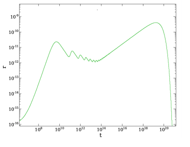
(a) Exact evolution.

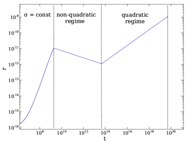
(b) Piecewise scaling-law approximation.

Figure 1: Comparison between the exact evolution and scaling-law approximation of the relative curvaton energy density. Here the parameters have been chosen to be $n=2$, $m=10^{-13}$ and $\Gamma=10^{-20}$, and the inital conditions $r_{*}=10^{-16}$ and $H_{*}=10^{-7}$. The three different phases of curvaton evolution can be clearly seen: First the energy density stays constant and hence $r\propto a^{4}$, then it starts to oscillate in the non-quadratic part and hence $r\propto a^{-1/2}$ until it enters the regime of quadratic oscillations where $r\propto a$. Decay occurs when $\Gamma=H$.

These three phases are clearly seen Fig. 1, which for a single choice of parameters displays the full numerical solution of evolution of $r=\rho_{\sigma}/\rho_{r}$, and then the piecewise scaling-law approximation, where we assume that when a single term dominates the potential, it scales according to Eq. (10) until $H\sim\Gamma$, and the curvaton decays instantaneously.

The more subdominant the curvaton is during its decay, the less efficiently the initial perturbation in the curvaton field is transmitted to metric fluctuations. However, since the curvaton is very subdominant during inflation, i.e. its field value is small, the quantum fluctuations produce relatively large perturbations when compared to the field value. Since the perturbation itself can be large, the curvaton does not need to be dominant at the decay. Instead, it is sufficient that its relative density grows enough from the given initial value. How much is ”enough” will be discussed in detail in Sect. 3.

2.3 Breakdown of the scaling law and oscillation of the curvature perturbation

From the qualitative discussion above, one would infer that the curvature perturbation varies smoothly and monotonously as the parameter values are changed. However, this is not quite true as the naïve use of the scaling law (10) does not capture all the relevant dynamical details.

When using the scaling law (10), one assumes the validity of two approximations: first, that a single term in the potential dominates completely; and second, that the oscillations are rapid when compared to the Hubble time $H^{-1}$. Neither of these assumptions is necessarily valid. The presence of two different terms in the potential (1) could be taken into account by generalizing the scaling law (10) following the methods outlined in [21]. This would not affect significantly the qualitative features of the results. The breakdown of the latter assumption of rapid oscillations can however have more significant effects. These can be seen in the numerical solutions of the equations of motion which exhibit complicated behaviour not qualitatively present in the simplified analytical approximation. To demonstrate this, in Fig. 2 we plot $\Delta N$ as a function of $H$ for fixed values of $H_{*}$, $r_{*}$ and $\Gamma$ for two different curvaton mass values. For different masses the moment of transition from the non-renormalizable part of the potential to the quadratic part of the potential is different, and this affects strongly the final value of $\Delta N$ which is dictated by the duration of oscillations in the non-quadratic regime.

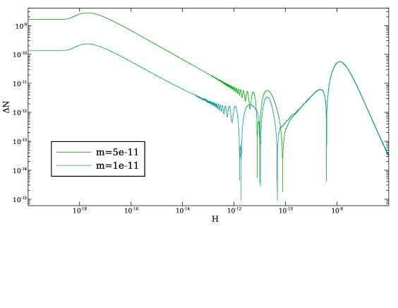
Figure 2: $\Delta N$ as a function of $H$, (time evolves from right to left). Both curves have $H_{*}=10^{-6}$, $n=4$, $\Gamma=10^{-18}$ and $r_{*}=10^{-10}$, but masses are for the lower one $m=10^{-11}$ and for the upper one $5\cdot 10^{-11}$. Here we demonstrate the non-trivial evolution of $\Delta N$. Deep in the quadratic regime its oscillations become faster and faster so that $\Delta N$’s evolution is given by a scaling law. However, before the quadratic term in the potential starts to dominate, $\Delta N$ shows very complicated oscillatory behaviour.

From Fig. 2 it is clear that as the field value oscillates in time, so does $\Delta N$. In the non-quadratic regime $\Delta N$ oscillates with a large amplitude. If the transition to the quadratic regime is slow compared to the oscillations in the non-quadratic regime, the transition averages over several oscillations. As a consequence, the final value of $\Delta N$ will be a non-oscillatory function of the model parameters. However, if the oscillation frequency in the non-quadratic potential is slow, and the transition to the quadratic oscillations is rapid, then the phase of the non-quadratic oscillation affects the final value of $\Delta N$. If the parameters happen to be such that the transition to the quadratic regime occurs at a maximum of the oscillation, a relatively high value of $\Delta N$ freezes out. Similarly, if the transition occurs at a minimum of the oscillation cycle, the final value of $\Delta N$ will be much smaller. If the parameters governing the moment of transition, such as the curvaton mass $m$, are changed continuously, then the phase of the non-quadratic oscillation during the transition also changes continuously. In the space of the parameters this results in an oscillatory pattern in $\Delta N$. This behaviour can be understood by observing that the curvaton energy density at the beginning of oscillations can not be expressed in terms of an amplitude of the envelope alone but also depends on the phase of the oscillation, or equivalently on both the field $\sigma$ and its time derivative $\dot{\sigma}$, in a non-trivial way. In effect, these act as two independent dynamical degrees of freedom. If the transition from the interaction dominated part to the quadratic region takes place at this stage, the initial variation of the curvaton value $\sigma_{*}$ can therefore translate in a non-trivial fashion into the final value of the curvature perturbation.

In [12] it was shown that for a potential $V\sim\sigma^{n+4}$ no oscillatory solutions exist if $n\geq 6$. This means that in the non-quadratic regime the curvaton merely decays and hence no oscillations in $\Delta N$ occur. This is consistent with the qualitative explanation of the oscillations discussed above.

3 Numerical solutions

3.1 Solving the equations of motion

We have explored the parameter space numerically for subdominant curvaton models that produce the curvature perturbation $\zeta\simeq 10^{-5}$ using the $\Delta N$ formalism with the patches defined as in Eq. (8).

The solution of the full equations of motion (2.1) oscillates more and more rapidly as it enters the regime dominated by the quadratic term in the potential. As each oscillation cycle requires several steps, solving the full equations of motion becomes increasingly slow as the rate of oscillations increase. To resolve this problem, we use the fact that deep in the quadratic regime the oscillations are very fast and hence the scaling law approximation Eq. (10) becomes very good. Formally this corresponds to taking $\langle\dot{\sigma}^{2}\rangle=\rho_{\sigma}$. Then we may switch from numerically evolving the equations of motion (2.1) to solving the energy density evolution equations

$$\dot{\rho_{\sigma}}=-\left(3H+\Gamma\right)\rho_{\sigma}$$ (12)

$$\dot{\rho_{\rm{r}}}=-4H\rho_{\rm{r}}+\Gamma\rho_{\sigma}$$

$$3H^{2}=\rho_{\rm{r}}+\rho_{\sigma} \,.$$

Since the solution of these equations does not have oscillatory behaviour, the step size can be increased significantly without sacrificing accuracy. Thus we choose to evolve the full system until the quadratic term dominates the non-quadratic term by a very large factor, e.g. $10^{5}$ for $n\geqslant 2$. This value is chosen for convenience only and ideally should be as large as possible. This is the point where the numerical integration of the equations of motion becomes intolerably slow, and the smaller $n$ in Eq. (1) is, the slower the numerics becomes. With $n=0$, the system should be followed through a very large number of oscillation cycles. Thus for $n=0$ we have to stop intregration already when the quadratic-to-non-quadratic ratio is $10^{2}$ to prevent the time of integration to grow to several minutes.

At this point, we switch to the evolution equations for the energy densities (12) and follow the system until the curvaton has decayed, i.e. radiation dominates the energy density of the curvaton by a very large factor, which we fix to be $10^{80}$. At this point we may compute the final value of $\Delta N$.

We are interested in how subdominant the curvaton is when it decays. This subdominance is described by the ratio of curvaton-to-radiation densities at the onset of decay, defined as

$$r_{\rm{decay}}=r(\Gamma\simeq H)~{}.$$ (13)

Since the value of $r_{\rm{decay}}$ is not an explicit parameter in the model, we calculate it by first solving the value for $\Gamma$ which gives the final amplitude of the perturbations to be the observed magnitude, $10^{-5}$. $r_{\rm{decay}}$ is then calculated with these parameters. Hence the result of the numerical simulations is a value for $r_{\rm{decay}}$ and $\Gamma$ for each parameter set $\{n,m,\lambda,H_{*},r_{*}\}$.

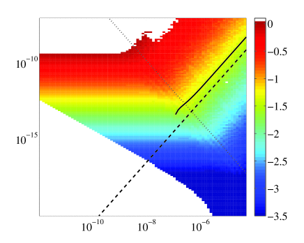
(a) $n=0$, $m=10^{-8}$

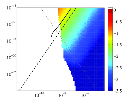
(b) $n=0$, $m=10^{-10}$

Figure 3: $\log_{10}r_{\rm{decay}}$ as a function of $H_{*}$ (horizontal axis) and $r_{*}$ (vertical axis) for $n=0$. The results are shown for a choice of coupling constant $\lambda=10^{-7}$. The white regions correspond to parameter values for which the amplitude of the curvature perturbation exceeds the observed value of $\zeta\sim 10^{-5}$, and are therefore immediately excluded. The characteristic value of the initial curvaton probability distribution $V(\sigma)\sim H^{4}/8\pi^{2}$ is indicated by the dashed line with high probability below the line, while the area below the solid line corresponds to the condition for nearly scale invariant spectrum $V^{\prime\prime}<10^{-2}H_{*}^{2}$. Below the dotted line non-quadratic terms in the potential are dynamically insignificant.

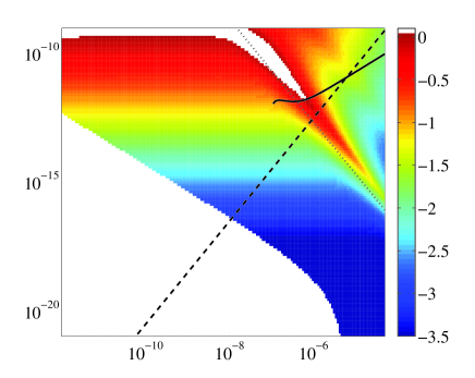
(a) $n=2$, $m=10^{-8}$

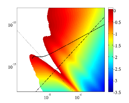
(b) $n=2$, $m=10^{-10}$

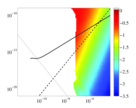
(c) $n=2$, $m=10^{-12}$

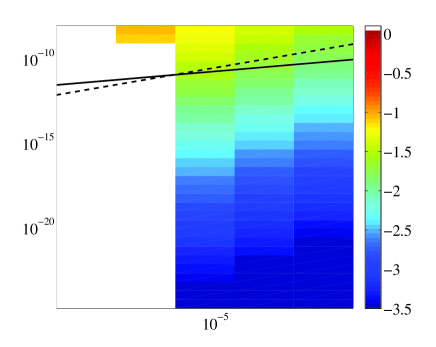
(d) $n=2$, $m=10^{-14}$

Figure 4: $\log_{10}r_{\rm{decay}}$ as a function of $H_{*}$ (horizontal axis) and $r_{*}$ (vertical axis) for $n=2$. The coupling constant is chosen to be $\lambda=1$. The white regions correspond to parameter values for which the amplitude of the curvature perturbation exceeds the observed value of $\zeta\sim 10^{-5}$, and are therefore immediately excluded. The characteristic value of the initial curvaton probability distribution $V(\sigma)\sim H^{4}/8\pi^{2}$ is indicated by the dashed line with high probability below the line, while the area below the solid line corresponds to the condition for nearly scale invariant spectrum $V^{\prime\prime}<10^{-2}H_{*}^{2}$. Below the dotted line non-quadratic terms in the potential are dynamically insignificant.

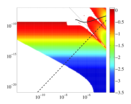
(a) $n=4$, $m=10^{-8}$

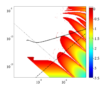
(b) $n=4$, $m=10^{-10}$

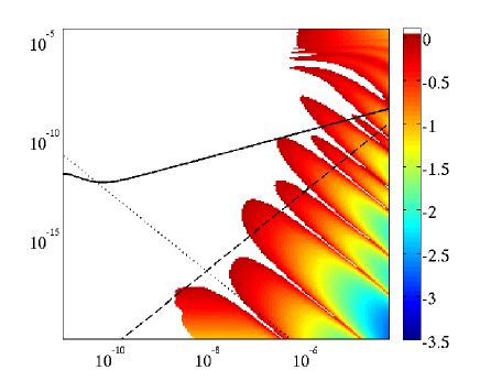
(c) $n=4$, $m=10^{-12}$

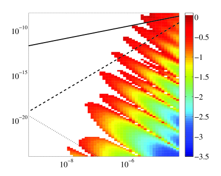
(d) $n=4$, $m=10^{-14}$

Figure 5: Same as in fig 4 but with $n=4$.

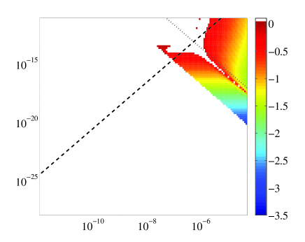
(a) $n=6$, $m=10^{-10}$

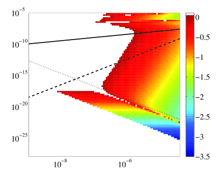
(b) $n=6$, $m=10^{-12}$

Figure 6: Same as in fig 4 but with $n=6$.

(a) $\log_{10}r_{\rm{decay}}$

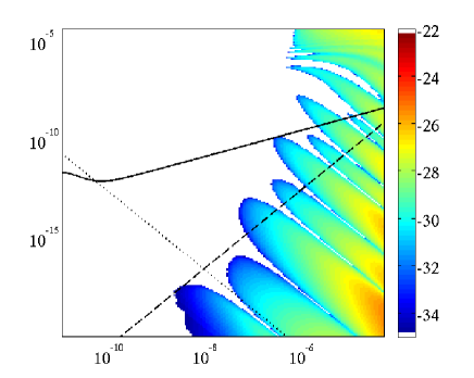
(b) $\log_{10}\Gamma$

Figure 7: $\log_{10}r_{\rm{decay}}$ and $\log_{10}\Gamma$ plotted as a function of $H_{*}$ (horizontal axis) and $r_{*}$ (vertical axis) for $m=10^{-12}$ and $n=4$. Lines as in previous figures.

3.2 Perturbation amplitude in parameter space

In Figs. 3 - 6 we have plotted $\log_{10}r_{\rm{decay}}$ with different choices of $n$ and $m$ as a function of $H_{*}$ and $r_{*}$. In addition to the value of $r_{\rm{decay}}$ we have plotted also the constraint for near scale invariance, $V^{\prime\prime}=10^{-2}H_{*}^{2}$ (solid line). The dotted line corresponds to the equality of the quadratic and non-quadratic terms in the potential during inflation; below the line the non-quadratic term has no sizeable effect. We also show the position of the edge of the curvaton probability distribution as given by Eq. (7) (dashed line); high probability is found below this line.

For $n>0$ we set $\lambda$ to unity, i.e. the cut-off scale to the Planck scale. We have, however, checked that decreasing $\lambda$ does not change the picture violently, but rather just moves the features seen in Figs. 4 - 6 slowly in the parameter space. For $n=0$, $\lambda$ is treated as a free parameter up to the constraint $\lambda\ll 1$ coming from the lightness of the curvaton in the interaction dominated regime.

The colder colors reflect a more subdominant curvaton and the warmer more dominant. The white color indicates that no matter how dominant the curvaton is, it cannot produce the observed amplitude of perturbations. The dominant curvaton scenario corresponds to the border between dark red and white, i.e. $r_{\rm{decay}}=1$. The numerical results demonstrate several features predicted by the simplified qualitative description discussed in sections 2.2 and 2.3.

The decay time is constrained from below by the requirement of no isocurvature perturbations, as discussed in Sect. 2.1. Adopting the limit on $\Gamma$ given in Eq. (4), some of the parameter space is ruled out; this is the source of the cutoff at the lower left corner of the figures.

Oscillations of the value of $r_{\rm{decay}}$ in the parameter space can be clearly seen. As discussed before, their source is the transition from the non-quadratic to the quadratic regime. Therefore, as expected, below the dotted line in the figures, where the non-quadratic term never dominates, the oscillations of $r_{\rm{decay}}$ are absent. Likewise, as there are no field oscillations in the $n=6$ potential, there are no ensuing oscillations of $r_{\rm{decay}}$ in the parameter space, as can be seen in Fig. 6. Furthermore, below the dotted line the value of $r_{\rm{decay}}$ depends only on $r_{*}$ and not on $H_{*}$. This is expected, since in the quadratic limit the relative curvaton perturbation is given by

$$\frac{\delta\sigma_{*}}{\sigma_{*}}=\frac{H_{*}/2\pi}{\sqrt{6r_{*}}H_{*}/m}=\frac{m}{2\pi\sqrt{6r_{*}}}\,.$$

Some of the parameter space of different curvaton models, as specified by $n$, and $m$, and by the inital conditions $r_{*}$ and $H_{*}$, is clearly ruled out. This is the white area in the plots. Large parts of the parameter space are however allowed, and for these areas, we have calculated the degree of subdominance at the time of curvaton decay. The figures clearly demonstrate that a curvaton model is feasible even when it is subdominant by a factor of $10^{-3}$ during decay. However, one should note that a very subdominant curvaton usually implies a large inflationary scale, as is also evident in the figures. This might not be a problem but as the inflationary scale grows the curvature perturbations generated during inflation also grow and can become significant [2] which needs to be taken into account in the analysis. For single field slow roll inflation, the inflaton perturbations are negligible if $H_{*}\ll 10^{-5}\sqrt{\epsilon_{*}}$.

The results given by the numerical code described above were also checked with an independently developed program, to verify that the features seen are not numerical errors.

4 Analytical results for $n=0$

4.1 Solving the equation of motion

The numerical results discussed in the previous section can be contrasted with an analytical estimate in the special case of $n=0$ for which we the potential (1) reads

$$V=\frac{1}{2}m^{2}\sigma^{2}+\lambda\sigma^{4}\ .$$ (14)

For this particular potential, it is possible to find a reasonably accurate analytical approximation for the exact solution of curvaton equation of motion. To some extent, the analysis serves as a useful consistency check of our numerical results, but can also be of certain interest of its own as it allows in principle to treat arbitrary values of the coupling $\lambda$ analytically.

In a radiation dominated background the equation of motion for a homogeneous curvaton with the potential (14) can be written as

$$\frac{{\rm d}^{2}f(a)}{{\rm d}a^{2}}+c_{1}f(a)^{3}+c_{2}a^{2}f(a)=0$$ (15)

where $a=(t/t_{*})^{1/2}$ is the scale factor, we have defined $f=a\sigma/\sigma_{*}$ and the star denotes the end of inflation. The constants are defined as $c_{1}=4\lambda\sigma_{*}^{2}/H_{*}^{2}$ and $c_{2}=m^{2}/H_{*}^{2}$. To identify $\sigma_{*}$ with the curvaton value at $t_{*}$, we should set the initial condition $\sigma(t_{*})=\sigma_{*}$. However, as the field is light at early times and evolves slowly, we choose instead to formally set the initial conditions $\sigma(t\rightarrow 0)=\sigma_{*}$ and $\dot{\sigma}(t\rightarrow 0)=0$ in the asymptotic past. This corresponds to

$$f(a)|_{a=0}=0\ ,~{}~{}f^{\prime}(a)|_{a=0}=1\ ,$$ (16)

and yields $\sigma(t_{*})=\sigma_{*}(1-{\cal O}(c_{1}))\simeq\sigma_{*}$, assuming $c_{1}>c_{2}$.

Exact solutions for Eq. (15) can be found if one of the constants $c_{1}$ and $c_{2}$ vanishes. In the absence of the quadratic term, $c_{2}=0$, the solution obeying the initial conditions (16) is given by the elliptic sine $f_{m=0}(a)=2^{1/4}c_{1}^{-1/4}{\rm sn}(2^{-1/4}c_{1}^{1/4}a,-1)$. This can be well approximated by the leading term of its trigonometric series

$$f_{m=0}(a)\simeq 2^{1/4}c_{1}^{-1/4}{\rm sin}(b\,2^{-1/4}c_{1}^{1/4}a)$$ (17)

with $b=\pi(2K(-1))^{-1}\simeq 1.1981$. The approximative solution obviously satisfies a differential equation obtained by setting $m=0$ in Eq. (15) and making the replacement $f(a)^{3}\rightarrow b^{2}c_{1}^{1/2}2^{-1/2}f(a)$.

This observation motivates us to study a much simpler linear equation

$$\frac{{\rm d}^{2}f(x)}{{\rm d}x^{2}}+\left(c+x^{2}\right)f(x)=0\ ,$$ (18)

instead of Eq. (15). Here a yet another redefinition of variables has been made

$$x=ac_{2}^{1/4}\ ,~{}~{}~{}~{}~{}~{}c=\frac{b^{2}\sqrt{2\lambda}\,\sigma_{*}}{m}\ .$$ (19)

Instead of the initial conditions (16) we need to impose

$$f(x)|_{x=0}=0\ ,~{}~{}f^{\prime}(x)|_{x=0}=bc_{2}^{-1/4}\ ,$$ (20)

to match with the desired exact solution of (15) in the limit $m\rightarrow 0$. By choosing the initial conditions (20) we implicitly restrict our analysis on the parameter values for which the quartic term is dominant or nearly dominant in (15) at early times, $c_{1}\gtrsim c_{2}$. Since Eq. (18) yields the correct approximative solution in the quartic limit $m\rightarrow 0$ and reduces to Eq. (15) at late times $x\gg 1$ when the quadratic term dominates the dynamics, we may expect it to yield a reasonable estimate for the asymptotic solutions of (15). Comparison with numerical results confirms that indeed this is the case, as illustrated in Fig. 8.

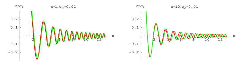
Figure 8: Comparison of the solutions for the curvaton field $\sigma=\sigma_{*}f(a)/a$ obtained from the exact equation (15) (green) and the approximative one (18) (red).

As can be seen, the solutions of Eqs. (18) and (15) differ by a slowly varying phase but the amplitudes agree quite well. This seems to be a generic outcome and not just a coincidence for the parameter values shown in Fig. 8. For our current purposes the phase difference is irrelevant as it would affect the curvature perturbation at late times $mt\gg 1$ only through terms suppressed by $m/H$ or $r$.

4.2 Asymptotic solution

The general solution for (18) can be expressed in terms of parabolic cylinder functions which admit simple asymptotic representations in the limit of large argument [22]. Focusing on late times $x=\sqrt{2mt}\gg c,~{}x\gg 1$, Eq. (18) yields the asymptotic result

$$\sigma_{\rm as}(t)\sim\frac{\sigma_{\rm osc}}{(mt)^{\frac{3}{4}}}\,{\rm sin}\left(mt+\frac{\pi}{8}+\delta\right)\ ,$$ (21)

where

$$\sigma_{\rm osc} = \sigma_{*}\frac{b\sqrt{\pi}e^{-\pi c/8}2^{-3/4}}{|\Gamma\left(\frac{3}{4}+i\frac{c}{4}\right)|}\ ,$$ (22)

$$\delta = \frac{c}{4}\,{\rm ln}(2mt)-{\arg}\left(\Gamma\left(\frac{3}{4}+i\frac{c}{4}\right)\right)\ ,$$ (23)

and the initial conditions (20) have been used. Fig. 9 shows a comparison between Eq. (21) and the exact solutions of (15) for the same parameter choices as in Fig. 8 but for later time events $x\gg c$ where the asymptotic solution is expected to be valid.

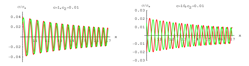
Figure 9: Comparison of the exact solution (green) for the curvaton field $\sigma=\sigma_{*}f(a)/a$ obtained from Eq. (15) and the asymptotic result (red) from Eq. (21).

Again it can be observed that the results are offset by a slowly varying phase difference, which manifests itself as the first term in Eq. (23), but the time evolution of the amplitude is well described by the asymptotic solution Eq. (21).

The dependence of $\sigma_{\rm osc}$ on the magnitude of the quartic term in Eq. (14) is illustrated in Fig 10.

Figure 10: The effective curvaton amplitude (22) $\sigma_{\rm osc}$ at the beginning of quadratic oscillations, $c\sim 2\sqrt{\lambda}\sigma_{*}/m$ measures the relative strength of the interaction term at the end of inflation.

For the interaction dominated case $c\gg 1$, Eq. (22) yields $\sigma_{\rm osc}\simeq\sigma_{*}c^{-1/4}2^{-3/4}b$ which according to (21) leads to an estimate $\bar{\sigma}\sim\sigma_{*}c^{-1/4}(H/m)^{3/4}$ for the envelope of oscillations in the quadratic regime. This is in agreement with the result obtained using the simple scaling law (10) and choosing $4\lambda\bar{\sigma}^{2}=m^{2}$ as the transition between quartic and quadratic regimes. In the limit $c\rightarrow 0$ where the quadratic term dominates throughout the evolution, $\sigma_{\rm osc}\rightarrow\sigma_{*}b\sqrt{\pi}2^{-3/4}/\Gamma(3/4)$ and Eq. (21) reduces to an asymptotic representation of a Bessel function. Up to the constant $b\simeq 1.1981$ related to the choice of initial conditions (20) engineered for the case $c\gtrsim 1$, this coincides with the exact solution for the quadratic case obeying the initial conditions (16).

4.3 Curvature perturbation

Using the result (21), the curvaton energy density at late times $mt\gg 1,~{}mt\gg c^{2}$ can be written as

$$\rho_{\sigma}\simeq\frac{m^{2}\sigma_{\rm osc}^{2}}{2(mt)^{3/2}}\left(1+{\cal{O}}(H/m)\right)\ .$$ (24)

The contribution from the quartic part of the potential (14) is negligible as equations (21) and (22) yield $\lambda\sigma^{2}/m^{2}\lesssim c^{2}/(mt)^{3/2}$. Neglecting the non-gravitational interactions between the curvaton and the dominant radiation component, the total energy density reads

$$\rho=\rho_{r*}a^{-4}+\rho_{\sigma}\ ,$$ (25)

where $\rho_{r*}\simeq 3H_{*}^{2}$ is the radiation energy density at the initial time $t_{*}$.

The curvature perturbation (9) at some time $t$ can be straightforwardly computed by varying (25) with respect to the initial curvaton value $\sigma_{*}$ and keeping the final energy density $\rho$ at $t$ fixed. To leading order in $r=\rho_{\sigma}/\rho_{r}$, this leads to the result

$$\zeta\simeq\frac{r}{2}\frac{\sigma_{\rm osc}^{\prime}}{\sigma_{\rm osc}}\delta\sigma_{*}+\frac{r}{4}\left(\frac{\sigma_{\rm osc}^{\prime\prime}}{\sigma_{\rm osc}}+\left(\frac{\sigma_{\rm osc}^{\prime}}{\sigma_{\rm osc}}\right)^{2}\right)\delta\sigma_{*}^{2}+\ldots=\sum_{n=1}^{\infty}\frac{\alpha_{n}}{n!}\delta\sigma_{*}^{n}\ ,$$ (26)

where

$$\alpha_{n}=\frac{r}{4\sigma_{\rm osc}^{2}}\sum_{m=0}^{n}\frac{n!}{m!(n-m)!}\frac{\partial^{n-m}\sigma_{\rm osc}}{\partial\sigma_{*}^{n-m}}\frac{\partial^{m}\sigma_{\rm osc}}{\partial\sigma_{*}^{m}}\ ,$$ (27)

and

$$r\simeq\frac{\sqrt{2}}{3}\,\sigma_{\rm osc}^{2}\left(\frac{m}{H}\right)^{1/2}\ .$$ (28)

The prime in (26) denotes differentiation with respect to $\sigma_{*}$ and the amplitude of perturbations is estimated by $\delta\sigma_{*}\sim H_{*}/(2\pi)$. In the sudden decay approximation, the curvaton is assumed to decay instantaneously at the time $H=\Gamma$ where, up to factors of unity, $\Gamma$ is given by the model dependent perturbative curvaton decay rate. The final value of the curvature perturbation under this assumption is obtained by setting $H=\Gamma$ in (26). Here we assume that the universe evolves adiabatically after the curvaton decay and hence $\dot{\zeta}=0$.

It is also straightforward to derive a formally non-perturbative expression for the curvature perturbation (see also [3]) which can be directly compared with our numerical results. By performing a finite shift $\sigma_{*}\rightarrow\sigma_{*}+\Delta\sigma_{*}$ in (25) but keeping the energy density $\rho$ fixed, we arrive at a fourth order equation for the curvature perturbation $\zeta={\rm ln}\,(a+\Delta a)-{\rm ln}\,a$

$$(1+r(\sigma_{*}))\,e^{4\zeta}-\frac{r(\sigma_{*})\sigma_{\rm osc}^{2}(\sigma_{*}+\Delta\sigma_{*})}{\sigma_{\rm osc}^{2}(\sigma_{*})}\,e^{\zeta}-1=0\ .$$ (29)

4.4 Comparing with numerical estimates

Equation (29 ) can be readily solved using standard methods. Qualitative features of the solutions are illustrated in Fig. 11 below, which shows $\zeta(\sigma_{*})$ for three different choices of the coupling $\lambda$ together with the corresponding numerical results.

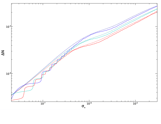
Figure 11: The curvature perturbation $\zeta$ for a choice of parameters $n=0$, $m=10^{-9}$, $H_{*}=10^{-7}$ and $\Gamma=10^{-28}$. The coupling values are $\lambda=10^{-7}$, $\lambda=2\times 10^{-7}$ and $\lambda=4\times 10^{-7}$ for red, green and blue curves respectively. The solid lines show numerical results and dashed lines analytical estimates.

First, we can observe that the agreement between analytical and numerical results is very good, even surprisingly so. The mismatch seen for small field values occurs where the dynamics is dominated by the quadratic potential $c\ll 1$ and the choice of initial conditions for our analytical computation is no longer valid, as discussed above. In this regime, we expect an error proportional to $b\sim 1.2$ which seems to be well in line with the behaviour seen in Fig. 11. The bump around $\sigma_{*}\sim 10^{-6}$ marks the regime where the quadratic and quartic terms are roughly equal initially, $c\sim 1$, and the transition from quartic to quadratic potential takes place soon after the onset of oscillations. For larger field values, oscillations in the quartic potential last for some while and the result can be understood using the simple scaling law (10). These features are generic although discussed here using the specific choice of parameters in Fig. 11 as an example.

Unlike for the non-renormalizable potentials, we do not detect any oscillatory behaviour of $\zeta$ in the regime $c\sim 1$ but instead only the bump. Indeed, using (29) we have checked that the first derivative of $\zeta$ with respect to $\sigma_{*}$ is a positive definite function in the limit $r\ll 1$ and non-monotonous features will show up only in third and higher order derivatives. This differs qualitatively from the non-renormalizable case where $\zeta$ oscillates as a function of $\sigma_{*}$ and consequently even $\zeta^{\prime}$ must change sign. Although we do not have an analytical estimate valid for non-renormalizable potentials, this agrees with general qualitative expectations as the transition into the quadratic regime takes place earlier due to the more rapid decrease of the field amplitude and is therefore more prone to leave an imprint on the perturbation.

Finally, using (26) we can express the amplitude of Gaussian perturbations and the non-linearity parameter $f_{\rm NL}=5/6({\rm ln}\,a)^{\prime\prime}/({\rm ln}\,a)^{\prime}{}^{2}$ to leading order in $r$ and up to numerical factors in the form

$$\zeta\sim\sigma_{*}\left(\frac{m}{\Gamma}\right)^{1/2}\delta\sigma_{*}\times f_{1}(c)\ ,~{}~{}f_{\rm NL}\sim\frac{1}{\sigma_{*}^{2}}\left(\frac{\Gamma}{m}\right)^{1/2}\times f_{2}(c)\ ,$$ (30)

which coincide with the well known quadratic results [4] apart from the functions $f_{1}=\sigma_{\rm osc}\sigma_{\rm osc}^{\prime}/\sigma_{*}$ and $f_{2}=(\sigma_{*}/\sigma_{\rm osc})^{2}(1+{\sigma_{\rm osc}\sigma_{\rm osc}^{\prime\prime}}/{\sigma_{\rm osc}^{\prime}{}^{2}})$. These depend only on the dimensionless parameter $c$ and their behaviour is depicted in Fig. 12.

Figure 12: $f_{1}$ and $f_{2}$ plotted for different values of $c\sim 2\sqrt{\lambda}\sigma_{*}/m$. $f_{1}$ and $f_{2}$, defined in Eq. (30), describe the deviation of $\zeta$ and $f_{\rm NL}$ from the purely quadratic results.

It can be seen that the inclusion of a quartic term in the potential tends to decrease the perturbation amplitude and enhance the non-Gaussian effects, except for the slight decrease of $f_{\rm NL}$ observed around $c\sim 1$. However, deviations from quadratic results are rather small as long as the quartic term is not vastly dominant over the quadratic part during inflation. For example, it can be seen from Fig. 12 that the quadratic results get modified by at most an order of magnitude for $c\lesssim 10$, where $c=10$ already corresponds to a clear dominance of the quartic term. In this regime the model is therefore compatible with observations under much of the same conditions as a quadratic model with the same parameters $(\sigma_{*},H_{*},m,\Gamma)$, although one also needs to take into account the different consistency constraints coming from the masslessness and subdominance of curvaton during inflation. If the interaction becomes more dominant, $c\gtrsim 10$ or so, Fig. 12 implies that the main constraints come from the observational upper bound $|f_{\rm NL}|\lesssim 100$ for the bispectrum [20]. This translates into a lower bound for the curvaton subdominance $r$, which will be more stringent than the quadratic result $r\gtrsim 0.01$ [4]. These limits from non-gaussianity need to be checked more carefully, and calculated also for the cases $n>0$ [23].

5 Conclusions

We have studied the evolution of the amplitude of primordial perturbation in a class of curvaton models where the potential contains, in addition to the usual quadratic term, either a quartic or some non-renormalizable term. For the calculation of the perturbation amplitude, these turn out to be dynamically important for a large part of the parameter space. We also focused on the possibility that the curvaton energy density is subdominant at the time of its decay. To some extent, this a natural consequence of non-renormalizable curvaton potential since then the relative curvaton energy density $r$ gets damped after inflation when the field is oscillating in the non-quadratic part of its potential. Depending on the decay time, this stage is followed by oscillations in a quadratic potential whence $r$ starts to increase again, but typically remains subdominant for realistic decay widths.

Although the amplification of curvaton energy is less efficient than for a quadratic model, the interacting model may still generate the observed amplitude of primordial perturbation since the initial curvaton perturbation $\delta\sigma_{*}/\sigma_{*}$ can be much larger than $10^{-5}$. This translates into constraints for the model parameters: the decay width $\Gamma$, the inflationary scale $H_{*}$, the bare curvaton mass $m$ and its initial energy density $r_{*}$. In the present paper we have performed a systematic study of the available parameter space for different types of non-quadratic potentials. We have shown that the correct amplitude of perturbations can indeed be achieved for large regions of the parameter space even if the interaction term dominates over the quadratic part and the curvaton would be subdominant by a factor of $r\sim 10^{-3}$ or so at the time of its decay.

Moreover, we found that the final relative curvaton energy density $r_{\rm decay}$ required to give rise to the observed amplitude depends on the model parameters in a highly complicated way and, for non-renormalizable potentials, shows oscillatory behaviour when the non-quadratic part dominates initially. The same oscillatory features show up when considering the curvature perturbation $\zeta$ as a function of the curvaton value $\sigma_{*}$ during inflation. Again, this happens for a large portion of the parameter space. We have traced this non-monotonous parametric dependence to the field dynamics taking place during the transition from the non-quadratic to the quadratic part of the potential. If the transition takes place soon after the beginning of oscillations, both $\sigma$ and $\dot{\sigma}$ act as independent dynamical variables and, consequently, variation of the initial conditions can leave a non-trivial imprint on the expansion history. If the non-quadratic term always remains subdominant such features are absent. Also for the renormalizable case $n=0$, the transition does not give rise to oscillatory behaviour but nevertheless leaves a clearly distinguishable mark in the results. This agrees with the analytical estimates we have derived for this special case.

Some parts of the parameter space that give rise to an acceptable perturbation amplitude are likely to be ruled out because they produce large non-Gaussianities. This is expected as we consider the subdominant limit $r\ll 1$ where the non-Gaussian effect are known to be large already for a quadratic model. However, because of the non-monotonic dependence $\zeta(\sigma_{*})$ observed for non-renormalizable potentials, it is not evident what the final non-Gaussianity turns out be in this case. Indeed, when considering the expansion (9) for the curvature perturbation, the non-monotonic behaviour implies that the sign of $({\rm ln}\,a)^{\prime\prime}$ is varying, barring any accidental cancellations. In certain regions of the parameter space we should therefore find a significant suppression for the non-linearity parameter $f_{\rm NL}\sim({\rm ln}\,a)^{\prime\prime}/({\rm ln}\,a)^{\prime}{}^{2}$ measuring the bispectrum amplitude. It is clear though that this qualitative argumentation cannot be pushed much further and a detailed survey of the parameter space is required to address the question of non-Gaussianity. This will be the topic of a forthcoming paper [23].

- [1] K. Enqvist and M. S. Sloth, Nucl. Phys. B 626 (2002) 395 hep-ph/0109214; D. H. Lyth and D. Wands, Phys. Lett. B 524, 5 (2002) Phys. Lett. B 524 (2002) 5 hep-ph/0110002; T. Moroi and T. Takahashi, Phys. Lett. B 522, 215 (2001) [Erratum-ibid. B 539, 303 (2002)] hep-ph/0110096; A. D. Linde and V. F. Mukhanov, Phys. Rev. D 56 (1997) 535 astro-ph/9610219; S. Mollerach, Phys. Rev. D 42 (1990) 313.
- [2] D. Langlois and F. Vernizzi, Phys. Rev. D 70 (2004) 063522 astro-ph/0403258; G. Lazarides, R. R. de Austri and R. Trotta, Phys. Rev. D 70 (2004) 123527 hep-ph/0409335; F. Ferrer, S. Rasanen and J. Valiviita, JCAP 0410 (2004) 010 astro-ph/0407300; T. Moroi, T. Takahashi and Y. Toyoda, Phys. Rev. D 72, 023502 (2005) hep-ph/0501007; T. Moroi and T. Takahashi, Phys. Rev. D 72, 023505 (2005) astro-ph/0505339; K. Ichikawa, T. Suyama, T. Takahashi and M. Yamaguchi, Phys. Rev. D 78, 023513 (2008) \arXivid0802.4138.
- [3] H. Assadullahi, J. Valiviita and D. Wands, Phys. Rev. D 76, 103003 (2007) \arXivid0708.0223; J. Valiviita, H. Assadullahi and D. Wands, \arXivid0806.0623.
- [4] D. H. Lyth, C. Ungarelli and D. Wands, Phys. Rev. D 67, 023503 (2003) astro-ph/0208055.
- [5] T. Moroi and T. Takahashi, Phys. Rev. D 66, 063501 (2002) hep-ph/0206026; D. H. Lyth and D. Wands, Phys. Rev. D 68 (2003) 103516 astro-ph/0306500; M. Beltran, Phys. Rev. D 78, 023530 (2008) \arXivid0804.1097; T. Moroi and T. Takahashi, Phys. Lett. B 671, 339 (2009) \arXivid0810.0189.
- [6] See e.g. L. Kofman and S. Mukohyama, Phys. Rev. D 77 (2008) 043519 \arXivid0709.1952.
- [7] K. Enqvist, S. Nurmi and G. I. Rigopoulos, JCAP 0810, 013 (2008) \arXivid0807.0382.
- [8] M. Bastero-Gil, V. Di Clemente and S. F. King, Phys. Rev. D 70 (2004) 023501 hep-ph/0311237.
- [9] K. Enqvist and S. Nurmi, JCAP 0510, 013 (2005) astro-ph/0508573.
- [10] K. Enqvist and T. Takahashi, JCAP 0809, 012 (2008) \arXivid0807.3069.
- [11] See e.g. K. Enqvist, A. Jokinen, S. Kasuya and A. Mazumdar, Phys. Rev. D 68, 103507 (2003) hep-ph/0303165; K. Enqvist, S. Kasuya and A. Mazumdar, Phys. Rev. Lett. 90, 091302 (2003) hep-ph/0211147; K. Enqvist, S. Kasuya and A. Mazumdar, Phys. Rev. Lett. 93, 061301 (2004) hep-ph/0311224; K. Enqvist, A. Mazumdar and A. Perez-Lorenzana, Phys. Rev. D 70, 103508 (2004) hep-th/0403044; M. Postma, Phys. Rev. D 67, 063518 (2003) hep-ph/0212005; S. Kasuya, M. Kawasaki and F. Takahashi, Phys. Lett. B 578, 259 (2004) hep-ph/0305134; R. Allahverdi, Phys. Rev. D 70 (2004) 043507 astro-ph/0403351; M. Ikegami and T. Moroi, Phys. Rev. D 70, 083515 (2004) hep-ph/0404253; R. Allahverdi, K. Enqvist, A. Jokinen and A. Mazumdar, JCAP 0610 (2006) 007 hep-ph/0603255.
- [12] K. Dimopoulos, G. Lazarides, D. Lyth and R. Ruiz de Austri, Phys. Rev. D 68 (2003) 123515 hep-ph/0308015.
- [13] Q. G. Huang, JCAP 0811 (2008) 005 \arXivid0808.1793.
- [14] N. Bartolo, S. Matarrese and A. Riotto, Phys. Rev. D 69, 043503 (2004) hep-ph/0309033; C. Gordon and K. A. Malik, Phys. Rev. D 69, 063508 (2004) astro-ph/0311102; K. A. Malik and D. H. Lyth, JCAP 0609, 008 (2006) astro-ph/0604387; M. Sasaki, J. Valiviita and D. Wands, Phys. Rev. D 74, 103003 (2006) astro-ph/0607627; J. Valiviita, M. Sasaki and D. Wands, astro-ph/0610001.
- [15] A. A. Starobinsky and J. Yokoyama, Phys. Rev. D 50, 6357 (1994) astro-ph/9407016.
- [16] D. S. Salopek and J. R. Bond, Phys. Rev. D 42 (1990) 3936.
- [17] A. A. Starobinsky, JETP Lett. 42 (1985) 152 [Pisma Zh. Eksp. Teor. Fiz. 42 (1985) 124]; M. Sasaki and E. D. Stewart, Prog. Theor. Phys. 95, 71 (1996); M. Sasaki and T. Tanaka, Prog. Theor. Phys. 99, 763 (1998).
- [18] D. Wands, K. A. Malik, D. H. Lyth and A. R. Liddle, Phys. Rev. D 62 (2000) 043527 astro-ph/0003278; D. H. Lyth and D. Wands, Phys. Rev. D 68, 103515 (2003) astro-ph/0306498; D. H. Lyth, K. A. Malik and M. Sasaki, JCAP 0505, 004 (2005) astro-ph/0411220; D. H. Lyth and Y. Rodriguez, Phys. Rev. Lett. 95 (2005) 121302 astro-ph/0504045.
- [19] C. L. Bennett et al., Astrophys. J. 464 (1996) L1 astro-ph/9601067.
- [20] E. Komatsu et al. [WMAP Collaboration], Astrophys. J. Suppl. 180, 330 (2009) \arXivid0803.0547.
- [21] M. S. Turner, Phys. Rev. D 28, 1243 (1983).
- [22] See e.g. I. S. Gradshteyn and I. M. Ryzhik “Table of Integrals, Series, and Products,” Academic Press Inc.,Third Printing, 1969.
- [23] K. Enqvist, S. Nurmi, G. I. Rigopoulos, O. Taanila and T. Takahashi, in preparation.