Perfect matchings
for the three-term Gale-Robinson sequences

Abstract.

In 1991, David Gale and Raphael Robinson, building on explorations carried out by Michael Somos in the 1980s, introduced a three-parameter family of rational recurrence relations, each of which (with suitable initial conditions) appeared to give rise to a sequence of integers, even though a priori the recurrence might produce non-integral rational numbers. Throughout the ’90s, proofs of integrality were known only for individual special cases. In the early ’00s, Sergey Fomin and Andrei Zelevinsky proved Gale and Robinson’s integrality conjecture. They actually proved much more, and in particular, that certain bivariate rational functions that generalize Gale-Robinson numbers are actually polynomials with integer coefficients. However, their proof did not offer any enumerative interpretation of the Gale-Robinson numbers/polynomials. Here we provide such an interpretation in the setting of perfect matchings of graphs, which makes integrality/polynomiality obvious. Moreover, this interpretation implies that the coefficients of the Gale-Robinson polynomials are positive, as Fomin and Zelevinsky conjectured.

In memory of David Gale, 1921-2008

1. Introduction

Linear recurrences are ubiquitous in combinatorics, as part of a broad general framework that is well-studied and well-understood; in particular, many combinatorially-defined sequences can be seen on general principles to satisfy linear recurrences (see [26]), and conversely, when an integer sequence is known to satisfy a linear recurrence it is often possible to reverse-engineer a combinatorial interpretation for the sequence (see [4] and references therein for a general discussion, and [3, Chapter 3] for specific examples). In contrast, rational recurrences such as

$$s(n)=(s(n-1)s(n-3)+s(n-2)^{2})/s(n-4),$$

which we prefer to write in the form

$$s(n)s(n-4)=s(n-1)s(n-3)+s(n-2)^{2},$$

are encountered far less often, and there is no simple general theory that describes the solutions to such recurrences or relates those solutions to combinatorial structures. The particular rational recurrence relation given above is the Somos-4 recurrence, and is part of a general family of recurrences introduced by Michael Somos:

$$s(n)s(n-k)=s(n-1)s(n-k+1)+s(n-2)s(n-k+2)+\cdots+s(n-\lfloor k/2\rfloor)s(n-\lceil k/2\rceil).$$

If one puts $s(0)=s(1)=\cdots=s(k-1)=1$ and defines subsequent terms using the Somos-$k$ recurrence, then one gets a sequence of rational numbers which for the values $k=4,5,6,7$ is actually a sequence of integers. (Sequences Somos-4 through Somos-7 are entries A006720 through A006723 in [24].) Although integer sequences satisfying such recurrences have received a fair bit of attention in the past few years, until recently algebra remained one step ahead of combinatorics, and there was no enumerative interpretation of these integer sequences. (For links related to Somos sequences, see http://jamespropp.org/somos.html.)

Inspired by the work of Somos, David Gale and Raphael Robinson [13, 12] considered sequences given by recurrences of the form

$$a(n)a(n-m)=a(n-i)a(n-j)+a(n-k)a(n-\ell),$$

with initial conditions $a(0)=a(1)=\cdots=a(m-1)=1$, where $m=i+j=k+\ell$. We call this the three-term Gale-Robinson recurrence . The Somos-4 and Somos-5 recurrences are the special cases where $(i,j,k,\ell)$ is equal to $(3,1,2,2)$ and $(4,1,3,2)$ respectively. Gale and Robinson conjectured that for all integers $i,j,k,\ell>0$ with $i+j=k+\ell=m$, the sequence $a(0),a(1),\dots$ determined by this recurrence has all its terms given by integers. About ten years later, this was proved algebraically in an influential paper by Fomin and Zelevinsky [11].

1.1. Contents

In this paper, we first give a combinatorial proof of the integrality of the three-term Gale-Robinson sequences. The integrality comes as a side-effect of producing a combinatorial interpretation of those sequences. Specifically, we construct a sequence of graphs $P(n;i,j,k,\ell)$ ($n\geq 0$) and prove in Theorem 9 that the $n$th graph in the sequence has $a(n)$ (perfect) matchings. Our graphs, which we call pinecones, generalize the well-known Aztec diamond graphs, which are the matchings graphs for the Gale-Robinson sequence 1, 1, 2, 8, 64, 1024, …  in which $i=j=k=\ell=1$. A more generic example of a pinecone is shown in Figure 1. All pinecones are subgraphs of the square grid.

\begin{picture}(2594.0,1394.0)(2979.0,-1208.0)\end{picture}

Figure 1. The pinecone $P(25;6,2,5,3)$. Its matching number is $a(25)$, where $a(n)$ is the Gale-Robinson sequence associated with $(i,j,k,\ell)=(6,2,5,3)$.

We give two ways to construct pinecones for the Gale-Robinson sequences: a recursive method (see Figure 11 and the surrounding text) that constructs the graph $P(n;i,j,k,\ell)$ in terms of the smaller graphs $P(n^{\prime};i,j,k,\ell)$ with $n^{\prime}<n$, and a direct method (see Formula (2) in Section 3) that allows one to construct the graph $P(n;i,j,k,\ell)$ immediately. The heart of our proof is the demonstration that if one defines $a(n)$ as the number of perfect matchings of $P(n)\equiv P(n;i,j,k,\ell)$, the sequence $a(0),a(1),a(2),...$ satisfies the Gale-Robinson recurrence. This fact, in combination with a simple check that $a(0)=a(1)=\cdots=a(m-1)=1$, gives an immediate inductive validation of our claim that $P(n)$ has $a(n)$ perfect matchings for all $n$, which yields additionally the integrality of $a(n)$.

General pinecones are defined in Section 2, where we also explain how to compute inductively their matching number via Kuo’s condensation lemma [17]. In Section 3, we describe how to associate a sequence of pinecones to a Gale-Robinson sequence, and observe that for these pinecones, the condensation lemma specializes precisely to the Gale-Robinson recurrence. Indeed, the recursive method of constructing pinecones, in combination with Kuo’s condensation lemma, gives combinatorial meaning to the different terms $a(n_{1})a(n_{2})$ of the Gale-Robinson recurrence.

In Section 4, we refine our argument to prove that the sequence $p(n)\equiv p(n;w,z)$ defined by

$$p(n)p(n-m)=w\,p(n-i)p(n-j)+z\,p(n-k)p(n-\ell),$$

with $i+j=k+\ell=m$ and $p(0)=p(1)=\cdots=p(m-1)=1$, is a sequence of polynomials in $w$ and $z$ with nonnegative integer coefficients. More precisely, we prove in Theorem 20 that $p(n;u^{2},v^{2})$ counts perfect matchings of the pinecone $P(n;i,j,k,\ell)$ by the number of special horizontal edges (the exponent of the variable $u$) and the number of vertical edges (the exponent of the variable $v$). The fact that $p(n)$ is a polynomial with coefficients in $\mathbb{Z}$ was proved in [11], but no combinatorial explanation was given and the non-negativity of the coefficients was left open.

1.2. Strategy, and connections with previous work

For much of the work in this paper, we share precedence with the students in the NSF-funded program REACH (Research Experiences in Algebraic Combinatorics at Harvard), led by James Propp, whose permanent archive is on the web at http://jamespropp.org/reach/. A paper by one of these students, David Speyer [25], introduced a very flexible framework (the “crosses and wrenches method”) that, starting from a recurrence relation of a certain type, constructs a sequence of graphs whose matching numbers satisfy the given recurrence. This framework includes the three-term Gale-Robinson recurrences, and thus yields a combinatorial proof of the integrality of the associated sequences. This extends to a proof that the bivariate Gale-Robinson polynomials mentioned above are indeed polynomials, and have non-negative coefficients. One difference with our paper is that Speyer’s graphs are only described explicitly for Somos-4 and Somos-5 sequences, whereas our construction is explicit for any Gale-Robinson sequence. Moreover, the description of our graphs as subgraphs of the square grid looks more regular, and may be useful to study limit shapes of random perfect matchings such as the perfect matchings shown in Figure 19.

Let us mention that shortly after Speyer did his work on perfect matchings, he and his fellow REACH-participant Gabriel Carroll did for four-term Gale-Robinson recurrences what Speyer had done for three-term Gale-Robinson recurrences, by introducing new objects called “groves” to take the place of perfect matchings [6]. Carroll and Speyer’s work gives, as two special cases, combinatorial proofs of the integrality of Somos-6 and Somos-7.

The strategies that led to Speyer’s article [25] and to the present article are not entirely independent; each made use of Propp’s prior construction of a suitable perturbed Gale-Robinson recurrence, which we explain next. The explanation will mostly be of interest to researchers seeking to apply similar techniques to other problems; others may want to skip the rest of the introduction.

Suppose we perturb a three-term Gale-Robinson recurrence by replacing the singly-indexed Gale-Robinson number $a(n)$ by a triply-indexed quantity $A(n,p,q)$ satisfying the perturbed recurrence

$$A(n,p,q)A(n-m,p,q)=A(n-i,p-1,q)A(n-j,p+1,q)+A(n-k,p,q+1)A(n-\ell,p,q-1).$$

(This choice of perturbation is not as special as it looks: all that matters is that the pairs $(-1,0),(1,0),(0,1),(0,-1)$ that describe the perturbations of the second and third coordinates in the four index-triples on the right-hand side, viewed as points in the plane, form a non-degenerate centrally-symmetric parallelogram. Choosing a different centrally-symmetric parallelogram is tantamount to a simple re-indexing of the recurrence.) If we take as our initial conditions $A(n,p,q)=x_{n,p,q}$ for all $n$ between 0 and $m-1$ and $p,q$ arbitrary, with (formal) indeterminates $x_{n,p,q}$, then each $A(n,p,q)$ with $n\geq m$ can be expressed as a rational function of these indeterminates. It should be emphasized here that for all $n,p,q,r,s$, the rational functions $A(n,p,q)$ and $A(n,r,s)$ are the same function up to re-indexing of the indeterminates.

Propp conjectured that each $A(n,p,q)$ is a Laurent polynomial in some finite subset of the (infinitely many) indeterminates $x_{n,r,s}$, with integer coefficients; that is, each $A(n,p,q)$ is an element of $\mathbb{Z}[x_{n,r,s}^{\pm 1}]$. This was subsequently proved by Fomin and Zelevinsky [11]. Note that if one sets all the indeterminates $x_{n,r,s}$ equal to 1, the Laurent polynomials $A(n,p,q)$ specialize to the Gale-Robinson numbers $a(n)$. Propp conjectured that each coefficient in each such Laurent polynomial is positive (a fact that is not proved by Fomin and Zelevinsky’s method) and furthermore is equal to $1$.

Propp knew that in the case $i=j=k=\ell=1$, the Laurent polynomials $A(n,p,q)$ can be interpreted as multivariate matching polynomials of suitable graphs, namely, the Aztec diamond graphs. (See Subsection 2.1 for a definition of matching polynomials.) Indeed, David Robbins had studied the three-parameter “perturbed recurrence” in this case, on account of its relation to the study of determinants, and had shown (with Rumsey) [22] that the associated rational functions are Laurent polynomials. (For more background on this connection with determinants, see [5].) The work by Elkies, Kuperberg, Larsen, and Propp [10] had shown that the monomials in these Laurent polynomials correspond to perfect matchings of Aztec diamond graphs. So it was natural to hope that this correspondence could be extended to the Gale-Robinson family of recurrences.

It should be acknowledged here that the idea behind the specific triply-indexed perturbation $A(n,p,q)$ of the Gale-Robinson sequence that proved so fruitful came from an article of Zabrodin [28] that was brought to Propp’s attention by Rick Kenyon. This article led Propp to think that the recurrence studied by Robbins should be considered a special case of the “discrete bilinear Hirota equation”, or “octahedron equation”, and that other recurrences such as the Gale-Robinson recurrence should likewise be considered in the context of the octahedron equation.

What the REACH students were able to do, after diligent examination of the Laurent polynomials $A(n,p,q)$, is view those Laurent polynomials as multivariate matching polynomials of suitable graphs. Bousquet-Mélou and West, independently, did the same for small values of $n$, until they were able to extrapolate these examples to the generic form of the graphs, which became the pinecones of this paper.

There is a general strategy here for reverse-engineering combinatorial interpretations of algebraically-defined sequences of numbers: add sufficiently many extra variables so that the numbers become Laurent polynomials in which every coefficient equals 1. For another application of this reverse-engineering method (in the context of Markoff numbers and frieze patterns), see [18].

2. Perfect matchings of pinecones

In this section we define a family of subgraphs of the square lattice, which we call pinecones. Then we prove that the number of perfect matchings of a pinecone can be computed inductively in terms of the number of perfect matchings of five of its sub-pinecones.

2.1. Preliminaries

To begin with, let us recall some terminology about graphs. A (simple) graph $G$ is an ordered pair $(V,E)$ where $V$ is a finite set of vertices, and $E$, the set of edges, is a collection of 2-element subsets of $V$. The degree of a vertex $v$ is the number of edges in $E$ containing $v$. A subgraph of $G$ is a graph $H=(V^{\prime},E^{\prime})$ such that $V^{\prime}\subset V$ and $E^{\prime}\subset E$. If, in addition, $V^{\prime}=V$, we say that $H$ is a spanning subgraph of $G$. The intersection of two graphs $G=(V,E)$ and $H=(V^{\prime},E^{\prime})$ is the graph $G\cap H=(V\cap V^{\prime},E\cap E^{\prime})$, and the union of the two graphs is the graph $G\cup H=(V\cup V^{\prime},E\cup E^{\prime})$. Given two graphs $G=(V,E)$ and $H=(V^{\prime},E^{\prime})$, we denote by $G\setminus H$ the subgraph $(V^{\prime\prime},E^{\prime\prime})$, where $V^{\prime\prime}=V\setminus V^{\prime}$ and $E^{\prime\prime}$ is the set of edges of $E\setminus E^{\prime}$ having both endpoints in $V^{\prime\prime}$.

A perfect matching of a graph $G=(V,E)$ is a subset $E^{\prime}$ of $E$ such that every vertex of $V$ belongs to exactly one edge of $E^{\prime}$. We will sometimes omit the word “perfect” and refer to perfect matchings as simply “matchings”. The matching number of $G$, denoted by $m(G)$, is the number of perfect matchings of $G$. More generally, we shall often consider the set $E$ of edges as a set of commuting indeterminates, and associate with a (perfect) matching $E^{\prime}$ the product of the edges it contains. The matching polynomial of $G$ is thus defined to be

$$M(G):=\sum_{E^{\prime}}\prod_{e\in E^{\prime}}e,$$

where the sum runs over all perfect matchings $E^{\prime}$ of $G$. If we replace every $e$ that occurs in this sum-of-products by a non-negative integer $n_{e}$, then this expression becomes a non-negative integer, namely, the number of perfect matchings of the multigraph in which there are $n_{e}$ edges joining the vertices $x$ and $y$ for all $e=\{x,y\}$ in $E$ (and no edges joining $x$ and $y$ if $\{x,y\}$ is not in $E$). In particular, if each $n_{e}$ is set equal to 0 or 1, then the matching polynomial becomes the number of perfect matchings of the subgraph of $G$ consisting of precisely those edges $e$ for which $n_{e}=1$.

Figure 2. An Aztec diamond graph of width $9$, and one of its perfect matchings.

2.2. Aztec diamonds graphs

The pinecones considered in this paper are certain subgraphs of the square lattice. The most regular of them are the (Aztec) diamond graphs, which are the duals of the so-called Aztec diamonds, which were first studied in detail in [10]. A diamond graph of width $2k-1$ is obtained by taking consecutive rows of squares, of length $1,3,\ldots,2k-3,2k-1,2k-3,\ldots,3,1$ and stacking them from top to bottom, with the middle squares in all the rows lining up vertically, as illustrated by Figure 2. Let $A$ be a diamond graph of width $2k-1$. Let $A_{N}$ be the diamond graph of width $2k-3$ obtained by deleting the leftmost and rightmost squares of $A$ as well as the two lowest squares of each of the remaining $2k-3$ columns of $A$. We call $A_{N}$ the North sub-diamond of $A$. Define similarly the South, West and East sub-diamonds of $A$, denoted by $A_{S},A_{W}$ and $A_{E}$. Finally, let $A_{C}$ be the central sub-diamond of $A$ of width $2k-5$ (Figure 3). The following result is a reformulation of Kuo’s condensation theorem for Aztec diamond graphs [17].

Figure 3. The five sub-diamonds of a diamond graph of width $9$.

Theorem 1 (Condensation for diamonds graphs).

The matching polynomial of a diamond graph $A$ is related to the matching polynomials of its sub-diamonds by

$$M(A)M(A_{C})=nsM(A_{W})M(A_{E})+ewM(A_{N})M(A_{S}),$$

where $n,s,w,$ and $e$ denote respectively the top (resp. bottom, westmost, eastmost) edge of $A$ (see Figure 2).

In particular, if $a(n)$ (with $n\geq 2$) denotes the matching number of a diamond graph of width $2n-3$, then

$$a(n)a(n-2)=2a(n-1)^{2}$$

for all $n\geq 2$, provided we adopt the initial conditions $a(0)=a(1)=1$. This shows that $a(n)$ is the three-term Gale-Robinson sequence associated with $i=j=k=\ell=1$, and implies $a(n)=2^{n\choose 2}$.

The condensation theorem we shall prove for pinecones appears as a generalization of the condensation theorem for diamond graphs. But it can actually also be seen as a specialization of it, and this is the point of view we adopt in this paper. The key idea is to forbid certain edges in the matchings.

Corollary 2.

Let $A$ be a diamond graph, and let $G$ be a spanning subgraph of $A$, containing the edges $n,s,w$ and $e$. Let $G_{N}=G\cap A_{N}$, and define $G_{S},G_{W},G_{E}$ and $G_{C}$ similarly. Then

$$M(G)M(G_{C})=nsM(G_{W})M(G_{E})+ewM(G_{N})M(G_{S}).$$

Proof.

Since $G$ is a spanning subgraph of $A$, every perfect matching of $G$ is a perfect matching of $A$. Hence the matching polynomial $M(G)$ is simply obtained by setting $a=0$ in $M(A)$, for every edge $a$ that belongs to $A$ but not to $G$. The same property relates $M(G_{N})$ and $M(A_{N})$, and so on. Consequently, Corollary 2 is simply obtained by setting $a=0$ in Theorem 1, for every edge $a$ that belongs to $A$ but not to $G$. ∎

2.3. Pinecones: definitions

A standard pinecone of width $2k-1$ is a subgraph $P=(V,E)$ of the square lattice satisfying the three following conditions, illustrated by Figure 4.$a$:

• The horizontal edges form $i+j+1$ segments of odd length, starting from the points $(0,1),(1,2)\ldots,(i-1,i)$ and $(0,0),(1,-1),\ldots,(-j,j)$, for some $i\geq 1$, $j\geq 0$. Moreover, if $L_{m}$ denotes the length of the segment lying at ordinate $m$, then

  $$L_{-j}<\cdots<L_{-1}<L_{0}=2k-1=L_{1}>L_{2}>\cdots>L_{i}.$$

• The set of vertices $V$ is the set of vertices of the square lattice that are incident to the above horizontal edges.

• Let $e=\{(a,b),(a,b+1)\}$ be a vertical edge of the square lattice joining two vertices of $V$. If $a+b$ is even, then $e$ belongs to the set of edges $E$, and we say that $e$ is an even edge of $P$. Otherwise, $e$ may belong to $E$, or not (Figure 4.$a$), and we call $e$ a (present or absent) odd edge.

The leftmost vertices of a standard pinecone are always $(0,0)$ and $(0,1)$. However, sometimes it is convenient to consider graphs obtained by shifting such a graph to a different location in the two-dimensional lattice. We will call such a graph a transplanted pinecone. In a transplanted pinecone, the leftmost vertices are $(a,b)$ and $(a,b+1)$, where $a+b$ is even. In some cases, where the distinction between standard and transplanted pinecones is not relevant or where we think the context makes it clear which sort of pinecone we intend, we omit the modifier and simply use the word “pinecone”.

Figure 4. Some pinecones of width $15$. $a$. The dashed edges may belong to the graph, or not. $b$. A pinecone. $c$. A closed pinecone.

Figures 4.$b$ and 4.$c$ show two specific ways to make the choices indicated in Figure 4.$a$ and obtain a pinecone of width 15. The pinecone of Figure 4.$c$ is closed, meaning that it contains no vertex of degree $1$. (Such a vertex can only occur at the right border of the pinecone, and occurs if the rightmost vertex of some horizontal segment does not belong to a vertical edge, as shown in Figure 4.$b$.) An Aztec diamond graph is an example of a closed pinecone. Let us color the cells of the square lattice black and white in such a way that the cell containing the vertices $(0,0)$ and $(1,1)$ is black. The faces of the pinecone are the finite connected components of the complement of the graph in $\mathbb{R}^{2}$. The faces of a pinecone $P$ are of three types: black squares, white squares, and horizontal rectangles consisting of a black cell to the left and a white cell to the right. We insist on the distinction between a cell (of the underlying square lattice) and a square (a face of $P$ that has 4 edges). For instance, the longest row of a pinecone of width $2k-1$ contains exactly $2k-1$ cells, but may contain no square at all. Denoting by $\ell$ (resp. $r$) the leftmost (resp. rightmost) cell of the longest row of $P$, we say that $P$ is rooted on $(\ell,r)$. (If $P$ is standard, then $\ell$ is the cell with $(0,0)$ as its lower-left corner.)

It is easy to see that a pinecone $P$ is closed if and only if the rightmost finite face of each row is a black square. In this case, the rightmost black square in each row is also the rightmost cell of the row. If moreover $P$ is standard, it is completely determined by the position of its black squares. Equivalently, it is completely determined by the position of its odd vertical edges. Conversely, consider any finite set $S$ of black squares whose lower-left vertices lie in the 90 degree wedge bounded by the rays $y=x>0$ and $-y=x>0$. Assume that $S$ is monotone, in the following sense: the rows that contain at least one square of $S$ are consecutive (say from row $-j$ to row $i$) and for $m>0$ (resp. $m<0$), the rightmost black square in row $m$ occurs to the left of the rightmost black square in row $m-1$ (resp. $m+1$). Then is a (unique) closed standard pinecone whose set of black squares is $S$.

We shall often consider the empty graph as a particular closed pinecone (associated with the empty set of black squares). The empty graph has one perfect matching, of weight 1.

2.4. The core of a pinecone

When a pinecone $P$ is not closed, some of the edges of $P$ cannot belong to any perfect matching of $P$. Specifically, if $v$ is a vertex of degree 1 in $P$, then in any perfect matching of $P$, $v$ must be matched with the vertex to its left (call it $u$), so that $u$ cannot be matched with any of its other neighbors. Indeed, there can be a chain reaction whereby a forced edge, in causing other edges to be forbidden, leads to new vertices of degree 1, continuing the process of forcing and forbidding other edges. An example of this is shown in Figure 5. The left half of the picture shows a non-closed pinecone $P$, and the right half of the picture shows a closed sub-pinecone $\bar{P}$ of $P$ along with a set of isolated edges. The reader can check (starting from the rightmost frontier of $P$ and working systematically leftward) that each of the isolated edges is a forced edge (that is, it must be contained in every perfect matching of $P$), so that a perfect matching of $P$ is nothing other than a perfect matching of $\bar{P}$ together with the set of isolated edges shown at right. In this subsection, we will give a systematic way of reducing a pinecone $P$ to a smaller closed pinecone by pruning away some forced and forbidden edges.

\begin{picture}(5091.0,1288.0)(429.0,-1230.0)\end{picture}

Figure 5. From a pinecone $P$ to its core $\bar{P}$.

It can easily be checked that the union or intersection of two standard pinecones is a standard pinecone, and that the union or intersection of two closed standard pinecones is a closed standard pinecone. It follows that, if $P$ is a standard pinecone, there exists a largest closed standard sub-pinecone of $P$, namely, the union of all the closed standard sub-pinecones of $P$. We call this the core of $P$ and denote it by $\bar{P}$. (If $P$ is not a standard pinecone but a transplanted pinecone rooted at the cell with lower-left corner $(a,b)$, we define $P_{0}$ as the standard pinecone obtained by translating $P$ by $(-a,-b)$, and we define the core of $P$ as the core of $P_{0}$ translated by $(a,b)$. However, for the rest of this section we will restrict attention to standard pinecones.)

Here is an alternative (more constructive and less abstract) approach to defining the core. Let $P$ be a standard pinecone. Let $b_{0}$ be the rightmost black square in row 0 of $P$, let $b_{1}$ be the rightmost black square in row 1 of $P$ that lies strictly to the left of $b_{0}$, let $b_{2}$ be the rightmost black square in row 2 of $P$ that lies strictly to the left of $b_{1}$, and so on (proceeding upwards); likewise, let $b_{-1}$ be the rightmost black square in row $-1$ of $P$ that lies strictly to the left of $b_{0}$, and so on (proceeding downwards). If at some point there is no black square that satisfies the requirement, we leave $b_{m}$ undefined. Consider all the faces of $P$ that lie in the same row as, and lie weakly to the left of, one of one of the $b_{k}$’s. This set of faces gives a closed pinecone $\tilde{P}$. At the same time, it is clear that any closed sub-pinecone $Q$ of $P$ must be a sub-pinecone of $\tilde{P}$. For, the rightmost black square in row 0 of $Q$ can be no farther to the right than $b_{0}$, which implies that the rightmost black square in row 1 of $Q$ can be no farther to the right than $b_{1}$, etc.; and likewise for the bottom half of $Q$. Hence the sub-pinecone $\tilde{P}$ we have constructed is none other than the core of $P$ as defined above.

If $P$ is closed, then $\bar{P}=P$. Note that a closed pinecone always admits two particularly simple perfect matchings: one consisting entirely of horizontal edges, and the other consisting of the leftmost and rightmost vertical edges in each row (and no other vertical edges) along with some horizontal edges (Figure 6). In particular, the rightmost vertical edges of a closed pinecone are never forced nor forbidden.

\begin{picture}(3763.0,988.0)(632.0,-780.0)\end{picture}

Figure 6. Two particularly simple matchings of a closed pinecone.

Let $P$ be a pinecone with core $\bar{P}$. There is a unique perfect matching of $P\setminus{\bar{P}}$ consisting exclusively of horizontal edges (see Figure 5); let $H$ be the edge set of this perfect matching. Every perfect matching of $\bar{P}$ can be extended to a perfect matching of $P$ by adjoining the edges in $H$, so $m(P)\geq m({\bar{P}})$. We now show that every perfect matching of $P$ is obtained from a perfect matching of $\bar{P}$ in this way.

Proposition 3.

Let $P$ be a pinecone with core $\bar{P}$. Then $m({\bar{P}})=m(P)$.

Proof.

We will prove this claim by using a procedure that reduces a sub-pinecone $Q$ of $P$ to a smaller sub-pinecone with the same matching number. Let $Q$ be a sub-pinecone of $P$ whose core coincides with $\bar{P}$. If $Q$ is not closed, then there must be at least one vertex of degree 1 along the right boundary of $Q$. Let $v=(a,b)$ be one of the the rightmost vertices of degree $1$ in $Q$. Then $v$ is the rightmost vertex in one of the rows of $Q$. Assume for the moment that $v$ lies strictly above the longest row of $Q$ (that is, $b>1$). See the top part of Figure 7 for an illustration of the following argument. Let $u$ be the vertex to the left of $v$. Then the edge joining $u$ and $v$ is forced to belong to every perfect matching of $Q$, while every other edge containing $u$ is forbidden from belonging to any perfect matching of $Q$. Hence the graph $Q^{\prime}$ obtained from $Q$ by deleting $u$, $v$, and every edge incident with $u$ or $v$ has the same matching number as $Q$. Furthermore, $Q^{\prime}$ is a pinecone, unless the vertex $v_{1}=(a-1,b+1)$ belongs to $Q$. In this case, $v_{1}$ has degree 1 in $Q^{\prime}$. Let $i$ be the largest integer such that $v_{j}=(a-j,b+j)$ belongs to $Q$ for all $0\leq j\leq i$. Applying the deletion procedure to the vertices $v=v_{0},v_{1},\ldots,v_{i}$ (in this order) yields a pinecone $Q^{*}$. Assume now that $b=1$. Applying the deletion procedure to all the vertices of $Q$ of the form $(a-j,1+j)$ or $(a-j,-j)$ yields again a pinecone $Q^{*}$ (see Figure 7, bottom). By symmetry, we have covered all possible values of $b$.

Figure 7. Some sequences of edge-deletions starting and ending with a pinecone.

Observe that $m(Q)=m(Q^{*})$. Additionally, we can check that the core of $Q^{*}$ is $\bar{P}$. The only thing we might worry about is that in passing from $Q$ to $Q^{*}$, we removed some edges that belong to $\bar{P}$. The examination of Figure 5 shows that we would have, in particular, removed the rightmost vertical edge is some row of $\bar{P}$. However, this cannot happen, because the removed edges were all forced or forbidden, whereas the rightmost edges of $\bar{P}$ are neither forced nor forbidden (Figure 6).

To prove that $m({\bar{P}})=m(P)$, take $Q=P$ and use the preceding operation repeatedly to construct successively smaller graphs $Q^{*}$, $Q^{**}$, …such that $m(P)=m(Q)=m(Q^{*})=m(Q^{**})=\cdots$ and $\bar{P}=\bar{Q}=\overline{Q^{*}}=\overline{Q^{**}}=\cdots\>$. Eventually we arrive at a closed sub-pinecone of $P$ whose core is $\bar{P}$; that is, we arrive at $\bar{P}$ itself. And since each step of our construction preserves $m(Q)$, we conclude that $m({\bar{P}})=m(P)$, as claimed. ∎

2.5. A condensation theorem for closed pinecones

Let $P$ be a closed pinecone, with longest row consisting of $2n+1$ squares. Let $A$ be the smallest diamond graph containing $P$ (the longest row of $A$ contains exactly $2n+1$ cells). Let $G$ denote the spanning subgraph of $A$ whose edge-set consists of all edges of $P$, all horizontal edges of $A$, and all even vertical edges of $A$ (Figure 8). Observe that $G$ is a pinecone. Moreover, among the spanning subgraphs of $A$ that are pinecones and contain $P$, $G$ has strictly fewer edges than the others. Since no odd vertical edge is added, $P$ is actually the core of the pinecone $G$.

Figure 8. Completing a pinecone $P$ into a spanning pinecone of an Aztec diamond graph.

Let us now use the notation of Corollary 2. That is, $G_{N}=G\cap A_{N}$, and so on. Then $G_{N},G_{S},G_{W},G_{E}$ and $G_{C}$ are (standard or transplanted) pinecones. Let $P^{N}$, $P^{S}$, $P^{W}$, $P^{E}$ and $P^{C}$ denote their respective cores. (These are not to be confused with $P_{N}$, etc., which are the intersections of $P$ with $A_{N}$, etc.) We will often call $P^{N}$, $P^{S}$, $P^{W}$, $P^{E}$ and $P^{C}$ “the five sub-pinecones” of $P$, even though, strictly speaking, $P$ admits other sub-pinecones. An example is given in Figure 9. Let $\ell_{0}$ (resp. $r_{0}$) be the leftmost (resp. rightmost) cell of the longest row $R_{0}$ of $P$. Similarly, let $r_{1}$ (resp. $r_{-1}$) denote the rightmost cell of the row just above (resp. below) $R_{0}$. Observe that the cells $r_{0},r_{1}$ and $r_{-1}$ correspond to black squares of $P$. Finally, let $\ell^{\prime}_{0}$ be the black cell of $R_{0}$ following $\ell_{0}$, and let $r^{\prime}_{0}$ the black square of $R_{0}$ preceding $r_{0}$ (if it exists). In light of the basic properties of the core (both the abstract definition and the algorithmic construction), we can give the following alternative description of the five sub-pinecones of $P$.

Figure 9. The five sub-pinecones of a pinecone $P$.

Proposition 4.

Let $P$ be a closed pinecone. With the above notation, $P^{N}$ (resp. $P^{S}$) is the largest closed sub-pinecone of $P$ whose rightmost cell is $r_{1}$ (resp. $r_{-1}$). Similarly, $P^{W}$ (resp. $P^{E}$) is the largest closed sub-pinecone whose rightmost (resp. leftmost) cell is $r^{\prime}_{0}$ (resp. $\ell^{\prime}_{0}$). Finally, $P^{C}$ is the largest closed sub-pinecone rooted on $(\ell^{\prime}_{0},r^{\prime}_{0})$.

This proposition implies that a pinecone $P$ that is neither empty, nor reduced to a black square can be reconstructed from its four main sub-pinecones $P^{N}$, $P^{S}$, $P^{E}$ and $P^{W}$. Indeed, the part of $P$ located strictly above its longest row coincides with the top part of $P^{N}$. More precisely, row $r$ of $P$, with $r>0$ coincides with row $r-1$ of $P^{N}$. Similarly, for $r<0$, row $r$ of $P$ coincides with row $r+1$ of $P^{S}$. It thus remains to determine the longest row of $P$. This row is obtained by adding a $2$-by-$1$ rectangle to the left of the longest row of $P^{E}$, and then superimposing the longest row of $P^{W}$.

Let us now apply Corollary 2 to the graph $G$ obtained by completing $P$ into a spanning pinecone of $A$ (Figure 8). By Proposition 3, since $P$ is the core of $G$, $m(G)=m(P)$, and similar identities relate the matching numbers of $G_{N}$ and $P^{N}$, etc.

Theorem 5 (Condensation for closed pinecones).

The matching number of a closed pinecone $P$ is related to the matching number of its closed sub-pinecones by

$$m(P)m(P^{C})=m(P^{W})m(P^{E})+m(P^{N})m(P^{S}).$$

We will state in Section 4 a more general condensation result dealing with the matching polynomial, rather than the matchings number, of closed pinecones (Theorem 13).

3. Pinecones for the Gale-Robinson sequences

The pinecones introduced in the previous section generalize Aztec diamond graphs. The number of perfect matchings of the diamond graph of width $2n-3$ is the $n$th term in the recurrence

$$a(n)a(n-2)=a(n-1)a(n-1)+a(n-1)a(n-1),$$

with initial conditions $a(0)=a(1)=1$. More generally, the three-term Gale-Robinson sequences are governed by recurrences of the form

$$a(n)a(n-m)=a(n-i)a(n-j)+a(n-k)a(n-\ell),$$ (1)

with initial conditions $a(n)=1$ for $n=0,1,\ldots,m-1$. Here, $i,j,k$ and $\ell$ are positive integers such that $i+j=k+\ell=m$, and we adopt the following (important) convention

$$j=\min\{i,j,k,\ell\}.$$

Our purpose in this section is to construct a sequence of (closed) pinecones $(P(n))_{n\geq 0}\equiv\left(P(n;i,j,k,\ell)\right)_{n\geq 0}$ for each set of parameters $\{i,j,k,\ell\}$ such that $i+j=k+\ell=m$, and to show that the matching numbers of the pinecones in our sequence satisfy the corresponding Gale-Robinson recurrence. More specifically, our family of graphs will be constructed in such a way that

• $P(n)^{C}$ is $P(n-m)$ transplanted to $(2,0)$ (that is, shifted two steps to the right),

• $P(n)^{W}$ is $P(n-i)$,

• $P(n)^{E}$ is $P(n-j)$ transplanted to $(2,0)$,

• $P(n)^{N}$ is $P(n-k)$ transplanted to $(1,1)$, and

• $P(n)^{S}$ is $P(n-\ell)$ transplanted to $(1,-1)$.

In our construction, we use the fact that a closed pinecone is completely determined by its set of odd vertical edges, that is, vertical edges of the form $\{(a,b),(a,b+1)\}$ where $a+b$ is odd. We introduce two functions, an upper function $U$ and a lower function $L$, which will be used to determine the positions of the odd vertical edges in the (closed) pinecone $P(n;i,j,k,\ell)$: for $r\geq 0$, let

$$\begin{array}[]{lll}U(n,r,c)&=&2c+r-3-2\left\lfloor{\displaystyle\frac{mc+kr+i-n-1}{j}}\right\rfloor,\\ \\ L(n,r,c)&=&2c+r-3-2\left\lfloor{\displaystyle\frac{mc+\ell r+i-n-1}{j}}\right\rfloor.\end{array}$$ (2)

Observe that the parameters $k$ and $\ell$ play symmetric roles. Also, $U(n,0,c)=L(n,0,c)$. The function $U$ will describe the upper part of the pinecone, while $L$ will describe its lower part. Recall that, by convention, the longest row of a standard pinecone is row $0$ and its South-West corner lies at coordinates $(0,0)$, as shown in Figure 4.

To locate the vertical odd edges in row $r\geq 0$, calculate the values $U(n,r,c)$ for $c=0,1,\ldots$ This will be a (strictly) decreasing sequence, since $m\geq 2j$ (recall that $i+j=m$ and $j\leq i$). Retain those values $U(n,r,c)$ that are larger than $r$, and place a vertical edge in the $r$th row at abscissa $U(n,r,c)$, that is, an edge connecting $(U(n,r,c),r)$ and $(U(n,r,c),r+1)$ (an odd edge, since $U(n,r,c)+r$ is odd). The first row not containing such an edge (and therefore not included in the pinecone) is the first one for which $U(n,r,0)<r$. Observe that $U(n,r,0)-r$ is a decreasing function of $r$ (since $j\leq k$). This property guarantees that if the $r$th row is empty, then all higher rows are empty too. It also implies that the rightmost vertical edge in row $r$ (which is located at abscissa $U(n,r,0)$) lies to the right of the rightmost vertical edge in row $r+1$. (To see this, note that $U(n,r,0)-r$ is always an odd number. So the inequality $U(n,r+1,0)-(r+1)<U(n,r,0)-r$ implies $U(n,r+1,0)-(r+1)\leq U(n,r,0)-r-2$, or $U(n,r+1,0)<U(n,r,0)$. That is, the set of odd edges (equivalently, of black squares) given by Formula (2) satisfies the “top part” of the monotonicity condition described at the end of Section 2.3: the rightmost odd edge in row $r>0$, if it exists, lies to the left of the rightmost odd edge in row $r-1$.

Similarly, to locate the edges in row $-r\leq 0$, calculate the values of $L(n,r,0)>L(n,r,1)>\cdots$ and retain those larger than $r$. For each, place a vertical edge in row $-r$ at abscissa $L(n,r,c)$, that is, connecting $(L(n,r,c),-r)$ and $(L(n,r,c),-r+1)$. Observe that $L(n,0,c)=U(n,0,c)$, so that the collection of odd vertical edges in row $0$ is the same whether it is determined from $U$ or from $L$.

The monotonicity properties satisfied by the positions of the odd edges imply that there exists a unique standard closed pinecone whose set of odd vertical edges coincides with the set we have constructed via the functions $U$ and $L$. To obtain this pinecone, draw horizontal edges from $(r,r+1)$ to $(U(n,r,0),r+1)$ and from $(-r,-r)$ to $(L(n,r,0),-r)$ for all $r\geq 0$. Finally, place all the appropriate even vertical edges. Since these steps are so routine, we regard the pinecone as fully described once the set of odd vertical edges has been specified. This point of view simplifies the exposition.

Observe that $P(n)$ is empty if and only if $U(n,0,0)<0$, which is equivalent to $U(n,0,0)\leq-1$ (since $U(n,0,0)$ is odd), which is easily seen to be equivalent to $n<m$ (using the fact that $m=i+j$).

Example. Take $(i,j,k,\ell)=(5,2,3,4)$ and determine $P(12)$. The above definition of $U$ and $L$ specializes to

$$U(n,r,c) = 2c+r-3-2\left\lfloor{\frac{7c+3r-8}{2}}\right\rfloor,$$

$$L(n,r,c) = 2c+r-3-2\left\lfloor{\frac{7c+4r-8}{2}}\right\rfloor.$$

In row $0$, we find odd edges with lower vertices $(5,0)$ and $(1,0)$. In row $1$, there is one odd edge at $(4,1)$. This is the top row of the diagram because $U(12,2,0)=1<2$. Turning to the lower portion of the diagram, there is one odd edge with lower vertex $(2,-1)$ and none in row $-2$ or below. Completing the diagram is now routine, and gives the pinecone $P(12)$ which is shown in Figure 10, together with its 14 perfect matchings. Accordingly, the Gale-Robinson sequence $a(n)$ associated with $(5,2,3,4)$ satisfies $a(12)=14$.

A larger example is presented after Corollary 10.

Figure 10. The pinecone $P(12;5,2,3,4)$, with black squares indicated, and its 14 perfect matchings (a cross stands for any of the two matchings of a square).

The pinecones based on the functions $U$ and $L$ satisfy a remarkable property: the odd edges (or, equivalently, the black squares) in rows $r$ and $r+1$ are interleaved. That is, between two black squares in row $r\geq 0$, there is a black square in row $r+1$, and similarly, between two black squares in row $r\leq 0$, there is a black square in row $r-1$. This can be checked on the small example of Figure 10, but is more visible on the bigger example of Figure 12.

Lemma 6 (The interleaving property).

For all values of $n,r$ and $c$, the functions $U$ and $L$ defined by (2) satisfy

$$U(n,r,c+1)+1\leq U(n,r+1,c)\leq U(n,r,c)-1$$

and

$$L(n,r,c+1)+1\leq L(n,r+1,c)\leq L(n,r,c)-1.$$

Proof.

We have

$$U(n,r+1,c)-U(n,r,c+1)=2\left\lfloor\frac{mc+kr+i-n-1+m}{j}\right\rfloor-2\left\lfloor\frac{mc+kr+i-n-1+k}{j}\right\rfloor-1.$$

But

$$\frac{mc+kr+i-n-1+m}{j}-\frac{mc+kr+i-n-1+k}{j}=\frac{\ell}{j}\geq 1,$$

so that the two floors occurring in the above identity differ by 1 at least. Consequently,

$$U(n,r+1,c)-U(n,r,c+1)\geq 2-1=1.$$

The three other inequalities are proved in a similar manner. ∎

We now wish to apply the condensation theorem (Theorem 5) to the pinecones $P(n)$ we have just defined. Using the notation of Theorem 5, we will verify that, up to translation, $P(n)^{W}=P(n-i)$, $P(n)^{E}=P(n-j)$, $P(n)^{N}=P(n-k)$, $P(n)^{S}=P(n-\ell)$ and $P(n)^{C}=P(n-m)$. These equivalences will follow from the interleaving property and the following algebraic equalities.

Lemma 7.

For any choice of parameters $(i,j,k,\ell)$, the functions $U$ and $L$ defined by (2) satisfy:

$$\begin{array}[]{rcllrcl}U(n-i,r,c-1)&=&U(n,r,c),&&L(n-i,r,c-1)&=&L(n,r,c),\\ U(n-j,r,c)&=&U(n,r,c)-2,&&L(n-j,r,c)&=&L(n,r,c)-2,\\ U(n-k,r-1,c)&=&U(n,r,c)-1,&\hskip 11.38109pt&L(n-\ell,r-1,c)&=&L(n,r,c)-1,\\ U(n-\ell,r+1,c-1)&=&U(n,r,c)-1,&&L(n-k,r+1,c-1)&=&L(n,r,c)-1,\\ U(n-m,r,c-1)&=&U(n,r,c)-2,&&L(n-m,r,c-1)&=&L(n,r,c)-2.\\ \end{array}$$

Proof.

The $L$-identities are symmetric to the $U$-identities upon exchanging $k$ and $\ell$, so that there are really 5 identities to prove. These can all be verified by routine algebraic manipulations. Let us check for instance the fourth identity satisfied by $U$:

$$U(n-\ell,r+1,c-1) = 2(c-1)+(r+1)-3-2\left\lfloor{\frac{m(c-1)+k(r+1)+i-(n-\ell)-1}{j}}\right\rfloor$$

$$= 2c+r-4-2\left\lfloor{\frac{mc+kr+i-n-1-m+k+\ell}{j}}\right\rfloor$$

$$= 2c+r-4-2\left\lfloor{\frac{mc+kr+i-n-1}{j}}\right\rfloor\hskip 34.1433pt\hbox{since }m=k+\ell$$

$$= U(n,r,c)-1.$$

We leave it to the reader to verify the remaining 4 identities. ∎

We now check that these identities imply that the pinecones are related to one another as claimed.

Proposition 8.

Let $P(n)\equiv P(n;i,j,k,\ell)$ be the sequence of pinecones associated with the parameters $(i,j,k,\ell)$. Then for $n\geq m$, the five closed sub-pinecones of $P(n)$ satisfy

$$P(n)^{W}=P(n-i), P(n)^{E}=P(n-j),$$

$$P(n)^{N}=P(n-k), P(n)^{S}=P(n-\ell),$$

and

$$P(n)^{C}=P(n-m).$$

These identities hold up to a translation.

Proof.

Begin by checking that $P(n)^{W}=P(n-i)$. Using the description of $P(n)^{W}$ given in Proposition 4, and the fact that the black squares of $P(n)$ are interleaved, we see that the odd vertical edges in $P(n)^{W}$ are those of $P(n)$, except that the rightmost odd edge in each row has been removed. (If this was the only odd edge in the row, then the entire row disappears.) Therefore $P(n)^{W}$ can be constructed by following the construction for $P(n)$, but beginning with $c=1,2,\ldots$ instead of $c=0,1,\ldots$. This means that in row $r\geq 0$ of $P(n)^{W}$, odd edges appear at positions $U(n,r,1),U(n,r,2),\ldots$ as long as these values continue to exceed $r$. (Similarly in rows $r\leq 0$, using $L$ instead of $U$.)

Let us now compare this with $P(n-i)$. In row $r\geq 0$ of $P(n-i)$, odd edges appear in positions $U(n-i,r,0),U(n-i,r,1),\ldots$, as long as these values continue to exceed $r$. However we showed in Lemma 7 that $U(n-i,r,c-1)=U(n,r,c)$, so the sequence of odd edges in row $r$ is the same in $P(n)^{W}$ and in $P(n-i)$. The situation is similar in rows $r<0$ using the equality for $L$. As we remarked above, a pinecone is determined by its odd edges (and the position of its leftmost edge), so $P(n)^{W}=P(n-i)$.

The other four equivalences are similar. The only new development is that instead of being positioned at the origin, the smaller pinecones are now offset by one or two columns (in all four cases) and possibly rows (in the case of $P(n)^{N}$ and $P(n)^{S}$). We will look at $P(n)^{S}$ as an example, and let the reader supply the details for the remaining three cases.

As noted after Proposition 4, for $r\leq 0$, row $r$ of $P(n)^{S}$ coincides with row $r-1$ of $P(n)$ (see Figure 9 for an example). For $r>0$, the leftmost cell of row $r$ of $P(n)^{S}$ lies two steps to the right of the leftmost cell of row $r-1$ of $P(n)$. Moreover, the interleaving property implies, by induction on $r$, that the last (i.e., rightmost) black square of row $r$ of $P(n)^{C}$ is the next-to last black square of row $r-1$ of $P(n)$. Thus the odd edges of $P(n)^{S}$ are located as follows: for rows $-r$, with $r=1,2,\ldots$, in columns $L(n,r,0),L(n,r,1),\ldots$, as long as these numbers continue to exceed $r$; and for rows $r=0,1,2,\ldots$, in columns $U(n,r,1),U(n,r,2),\ldots$, as long as these numbers continue to exceed $r+2$.

Let us now look at a copy of $P(n-\ell)$ positioned with its origin at $(1,-1)$. After this translation, the odd vertical edges in rows $-r$, with $r=1,2,\ldots$ are located at abscissas $L(n-\ell,r-1,c)+1$, for $c\geq 0$ and as long as these numbers continue to exceed $r$. Lemma 7 then implies that the bottom parts of $P(n)^{S}$ and of the translate of $P(n-\ell)$ coincide. After the translation, the odd vertical edges of $P(n-\ell)$ lying in rows $r$, with $r=0,1,2,\ldots$ are located at abscissas $U(n-\ell,r+1,c)+1$, for $c\geq 0$ and as long as these numbers continue to exceed $r+2$. Lemma 7 then implies that the top parts of $P(n)^{S}$ and of the translate of $P(n-\ell)$ coincide.

This completes the analysis for $P(n)^{S}$; the verifications for $P(n)^{N}$, $P(n)^{E}$ and $P(n)^{C}$ are similar (and even identical, up to symmetry, in the case of $P(n)^{N}$). ∎

Figure 11. Recursive graphical construction of the pinecones associated with the Somos-4 sequence. At each stage, one (or two) of the components that are superimposed to form the pinecone is highlighted.

Remark: a recursive construction of the pinecones $P(n)$. The above proposition, combined with Proposition 4, provides an alternative way of constructing the sequence of pinecones $P(n)$ associated with a given set of parameters $(i,j,k,\ell)$. For $0\leq n<m$, we put $P(n)$ equal to the empty graph (which has one perfect matching), and for $m\leq n<m+j$, we put $P(n)$ equal to the graph with four vertices and four edges surrounding one square face (which has 2 perfect matchings). Then, for $n\geq m+j$, it suffices to superimpose $P(n-i),P(n-j),P(n-k)$ and $P(n-\ell)$, and add a $2$-by-$1$ rectangle to the left of the longest row of $P(n-j)$. More precisely, the four above pinecones must be positioned in such a way the leftmost cell of $P(n-i)$ (resp. $P(n-j),P(n-k),P(n-\ell)$) has its South-West corner at $(0,0)$ (resp. $(2,0)$, $(1,1)$, $(1,-1)$), while the $2$-by-$1$ rectangle has its South-West corner at $(0,0)$. (This rectangle is only needed if $P(n-i)$ is empty or consists of a single black square. Typically this 2-by-1 rectangle comes for free as part of $P(n-i)$. Note that we do not claim that this rectangle is a face of the pinecone; the odd edge joining $(1,0)$ and $(1,1)$ will be present or absent in $P(n)$, according to whether it is present or absent in $P(n-i)$.) This gives a graphical, inductive way of constructing $P(n)$. This method is illustrated in Figure 11 by the case of the Somos-4 sequence, for which

$$a(n)a(n-4)=a(n-3)a(n-1)+a(n-2)^{2}.$$

That is, $(i,j,k,\ell)=(3,1,2,2)$ and $m=4$.

We can now state our combinatorial interpretation of the Gale-Robinson numbers.

Theorem 9.

Let $P(n)\equiv P(n;i,j,k,\ell)$ be the sequence of pinecones associated with the parameters $(i,j,k,\ell)$. Let $a(n)$ denote the number of perfect matchings of $P(n)$. Then $a(n)=1$ for $n<m$, and for $n\geq m$, the sequence $a(n)$ satisfies the following Gale-Robinson recurrence:

$$a(n)a(n-m)=a(n-i)a(n-j)+a(n-k)a(n-\ell).$$

Proof.

We have already observed that the pinecone $P(n)$ is empty for $n<m$. Hence the initial conditions apply correctly. Now for $n\geq m$, Theorem 5 states that the matching matching of $P(n)$ is related to the matching numbers of its closed sub-pinecones by

$$m(P(n))m(P(n)^{C})=m(P(n)^{W})m(P(n)^{E})+m(P(n)^{N})m(P(n)^{S}).$$

Proposition 8 then implies that $m(P(n)^{C})=m(P(n-m))$, etc. Therefore,

$$m(P(n))m(P(n-m))=m(P(n-i))m(P(n-j))+xm(P(n-k))m(P(n-\ell)),$$

which is the recurrence relation satisfied by $a(n)$. ∎

Before we study a specific example, let us state an obvious corollary of Theorem 9.

Corollary 10.

Let $i,j,k,\ell$ be positive integers such that $i+j=k+\ell=m$. The recurrence relation

$$a(n)a(n-m)=a(n-i)a(n-j)+a(n-k)a(n-\ell),$$

with initial conditions $a(n)=1$ for $n<m$, defines a sequence of positive integers

Example. We give a specific example in the case where $(i,j,k,\ell)$ = $(6,2,5,3)$ and $n=25$. We also show how to use the VAXmaple software package (available at http://jamespropp.org/vaxmaple.c) to compute the number of perfect matchings in the constructed pinecone, which can be seen to be the $25$th term in the appropriate Gale-Robinson sequence.

Considering first the upper portion of $P(n)$, we fix $r$ and then consider the first few values of $U(n,r,c)$ as $c=0,1,2,3,\ldots$:

$$r=0: \{17,11,5,-1,\ldots\}$$

$$r=1: \{14,8,2,-4,\ldots\}$$

$$r=2: \{9,3,-3,-9,\ldots\}$$

$$r=3: \{6,0,-6-12,\ldots\}$$

$$r=4: \{1,-5,-11,-17,\ldots\}$$

Since the $c=0$ value for $r=4$ is already less than $r$, there are only three non-empty rows above the middle (longest) row in this pinecone. For the lower portion of the diagram, we obtain the following values of $L(n,r,c)$:

$$r=0: \{17,11,5,-1,\ldots\}$$

$$r=1: \{16,10,4,-4,\ldots\}$$

$$r=2: \{13,7,1,-5,\ldots\}$$

$$r=3: \{12,6,0,-6,\ldots\}$$

$$r=4: \{9,3,-3,-9,\ldots\}$$

$$r=5: \{8,2,-4,-10,\ldots\}$$

$$r=6: \{5,-1,-7,-13,\ldots\}$$

Completing the construction, we arrive at the graph of Figure 12.

\begin{picture}(2594.0,1394.0)(2979.0,-1208.0)\end{picture}

Figure 12. The pinecone $P(25;6,2,5,3)$.

It is easy to translate this into the format required by the computer program VAXmaple, written by Greg Kuperberg, Jim Propp and David Wilson to count perfect matchings of finite subgraphs of the infinite square grid. In this format, each vertex present in the graph is represented by a letter. The choice of letter indicates whether any edges are omitted when connecting the vertex to its nearest neighbours — each vertex having up to four of these. An X indicates that no edges are omitted; an A indicates that the edge leading upward from the vertex is omitted; a V indicates the omission of the downward edge. (For a more detailed explanation of the software, see http://jamespropp.org/vaxmaple.doc.) The encoding of the pinecone of Figure 12 is given in Figure 13.

                                 XVXX
                                XXAVXVXX
                               XXXVAVAXXVXVXX
                              XVXVAXAVXVAXAVXVXX
                              XAVAXXVAVAXXVAVAXX
                               XAVXVAXAVXVAXAXX
                                XAVAXXVAVAXX
                                 XAVXVAXVXX
                                  XAVAXX
                                   XAXX

Figure 13. The pinecone $P(25;6,2,5,3)$ as a VAX file.

Counting the perfect matchings in this pinecone by running the above input through the VAXmaple program and then through Maple produces 167,741, as it should, since the $25$th term of the Gale-Robinson sequence constructed from $(6,2,5,3)$ is 167,741.

4. The Gale-Robinson bivariate polynomials

As stated in Corollary 10, Theorem 9 implies that the three-term Gale-Robinson sequences consist of integers. In this section, we refine this result as follows.

Theorem 11.

Let $i,j,k,\ell$ and $m$ be positive integers such that $i+j=k+\ell=m$. Let $w$ and $z$ be two indeterminates, and define a sequence $p(n)\equiv p(n;w,z)$ by $p(n)=1$ for $n<m$ and for $n\geq m$,

$$p(n)p(n-m)=w\,p(n-i)p(n-j)+z\,p(n-k)p(n-\ell).$$

Then $p(n)$ is a polynomial in $w$ and $z$ with nonnegative integer coefficients.

The proof goes as follows: we have already seen that $p(n;1,1)$ counts perfect matchings of the pinecone $P\equiv P(n;i,j,k,\ell)$ constructed in Section 3. We will prove that $p(n;u^{2},v^{2})$ counts these matchings according to two parameters. More precisely, we begin by giving in Section 4.1 a condensation theorem that computes inductively the matching polynomial (rather than the matching number) of closed pinecones. We observe that this theorem takes a simpler form when applied to interleaved pinecones (a class of pinecones that contains all Gale-Robinson pinecones). In Section 4.2, we define the special horizontal edges of a pinecone. We then define the partial matching polynomial of a pinecone $P$ as the matching polynomial $M(P)$ in which the weights of non-special edges are set to 1. We specialize the condensation theorem of Section 4.1 to a condensation theorem for the partial matching polynomial of interleaved pinecones. Its application to the Gale-Robinson pinecones $P(n;i,j,k,\ell)$ implies that the polynomial $q(n)\equiv q(n;u,v)$ that counts perfect matchings of $P(n)$ according to the number of vertical edges (the exponent of $v$) and horizontal special edges (the exponent of $u$) satisfies $q(n)=1$ for $n<m$ and

$$q(n)q(n-m)=u^{2}q(n-i)q(n-j)+v^{2}q(n-k)q(n-\ell)$$

for $n\geq m$. This shows that $q(n;u,v)=p(n;u^{2},v^{2})$ and implies Theorem 11.

4.1. A condensation theorem for the matching polynomial

Let us go back to the condensation theorem for closed pinecones (Theorem 5). We now state and prove a stronger result dealing with the matching polynomial rather than the matching number. Let $P$ be a closed pinecone and $A$ the smallest diamond graph that contains it, with $G$ defined as in the beginning of Section 2.5 and with $n$, $s$, $e$, $w$ as in Theorem 1 and Figure 2. Since $P$ is the core of $G$, the matching polynomial $M(G)$ equals $M(P)M(G\setminus P)$. Similar results hold for the sub-pinecones $P^{C}$, $P^{W}$, $P^{E}$, $P^{N}$ and $P^{S}$. Corollary 2 gives:

$$M(P)M(G\setminus P)M(P^{C})M(G_{C}\setminus P^{C})=nsM(P^{W})M(G_{W}\setminus P^{W})M(P^{E})M(G_{E}\setminus P^{E})\\ +ewM(P^{N})M(G_{N}\setminus P^{N})M(P^{S})M(G_{S}\setminus P^{S}).$$ (3)

Since $P$ is the core of $G$, the graph $G\setminus P$ has a unique perfect matching, which is formed of horizontal edges only. Hence $M(G\setminus P)$ is a monomial. The same holds for the other graph differences occurring in (3). We can thus rewrite this identity as

$$M(P)M(P^{C})=\alpha M(P^{W})M(P^{E})+\beta M(P^{N})M(P^{S})$$

for some Laurent monomials $\alpha$ and $\beta$ (indeed, negative exponents may arise from the division by $M(G\setminus P)M(G_{C}\setminus P^{C})$). Our objective in this subsection is to prove that these monomials only involve nonnegative exponents (so that they are ordinary monomials), and to describe them in a more concise way.

We introduce the following definition, illustrated in Figure 14.

Definition 12.

Let $P$ be a closed pinecone. A horizontal edge is a left edge if it is the leftmost horizontal edge in the horizontal segment of $P$ that contains it.

A horizontal edge with leftmost vertex $(i,j)$ is even if $i+j$ is even, odd otherwise.

\begin{picture}(2316.0,1288.0)(407.0,-855.0)\end{picture}

Figure 14. The left edges of a closed pinecone.

For a (standard) pinecone $P$, we denote by $P_{\geq}$ (resp. $P_{>}$) the pinecone formed of rows $0,1,2,\ldots$ of $P$ (resp. rows $1,2,\ldots$). We use similar notations for the bottom part of $P$. These definitions are extended to transplanted pinecones in a natural way: for instance, $(P^{N})_{\geq}$, which we simply denote $P^{N}_{\geq}$, consists of rows $1,2,\ldots$ of $P$.

Figure 15. The inclusion properties $P^{N}_{<}\subset P^{C}_{\leq}$ and $P^{C}_{>}\subset P^{N}_{\geq}$ (the small subpinecones are dashed). The leftmost figure also shows some edges of the horizontal matching of $P^{C}_{\leq}\setminus P^{N}_{<}$.

Observe that, for any pinecone $P$,

$$P^{N}_{<}\subset P^{C}_{\leq}\quad\hbox{ while }\quad P^{C}_{>}\subset P^{N}_{\geq}.$$ (4)

Both properties are illustrated in Figure 15. Consequently, the graph difference $P^{C}\setminus P^{N}$ is formed of edges that lie in $P_{\leq}^{C}$, and $P^{C}\setminus P^{N}\subset P^{C}_{\leq}\setminus P^{N}_{<}$. Let us describe more precisely the horizontal edges of these two graph differences. For $j\leq 1$, if there are any horizontal edges of $P^{C}_{\leq}\setminus P^{N}_{<}$ lying at ordinate $j$, then the number of them is odd, say $2k_{j}+1$, and these edges are the $2k_{j}+1$ rightmost horizontal edges of $P^{C}$ found at ordinate $j$ (Figure 15, left). If $j\leq 0$, all these edges belong to $P^{C}\setminus P^{N}$. However, for $j=1$, only a subset of these edges, of even cardinality, belong to $P^{C}\setminus P^{N}$. (In the example of Figure 15, the two leftmost thick edges shown at ordinate 1 do not belong to $P^{C}\setminus P^{N}$.) The graph $P^{C}_{\leq}\setminus P^{N}_{<}$ thus has a unique horizontal matching, which has $k_{j}+1$ edges at ordinate $j\leq 1$. We denote by $H^{-}(P^{C}\setminus P^{N})$ the product of the edges of this matching having ordinate $\leq 0$. The fact that the horizontal edges of $P^{C}\setminus P^{N}$ found at ordinate $j$ coincide with those of $P^{C}_{\leq}\setminus P^{N}_{<}$ allows us to use the notation $H^{-}(P^{C}\setminus P^{N})$ rather than something like $H^{-}(P^{C}_{\leq}\setminus P^{N}_{<})$ which would have been heavier.

Symmetrically,

$$P^{S}_{>}\subset P^{C}_{\geq}\quad\hbox{ while }\quad P^{C}_{<}\subset P^{S}_{\leq},$$ (5)

so that the graph $P^{C}\setminus P^{S}$ lies in $P_{\geq}^{C}$. We denote by $H^{+}(P^{C}\setminus P^{S})$ the product of the edge-weights of the horizontal matching of $P^{C}_{\geq}\setminus P^{S}_{>}$ lying at a positive ordinate.

Figure 16. Left: The edges occurring in the first term of the refined condensation theorem, with the pinecone $P^{W}$ shown. Right: The edges occurring in the second term. Here $H^{+}(P^{C}\setminus P^{S})=1$. The two distinguished pinecones are $P^{C}$ and $P^{N}$ (dashed).

We can now state a condensation theorem for the matching polynomial of closed pinecones. See Figure 16 for an illustration.

Theorem 13 (The matching polynomial of closed pinecones).

The matching polynomial of a closed pinecone $P$ is related to the matching polynomial of its sub-pinecones by

$$M(P)M\left(P^{C}\right)=\left(\prod_{a\in E_{1}}a\right)M\left(P^{W}\right)M\left(P^{E}\right)\\ +\left(\prod_{a\in E_{2}}a\right)H^{-}(P^{C}\setminus P^{N})H^{+}(P^{C}\setminus P^{S})M\left(P^{N}\right)M\left(P^{S}\right),$$

where

• $E_{1}$ is the set of left edges of $P$ not belonging to $P^{W}$,

• $E_{2}$ is the union of three edge-sets $E_{2}^{i}$, for $0\leq i\leq 2$:

  • $E_{2}^{0}=\{e,w\}$ contains the eastmost and westmost vertical edges of $P$,

  • $E_{2}^{1}$ contains the even edges at ordinate $1$ not belonging to $P^{N}$,

  • $E_{2}^{2}$ contains the odd edges at ordinate $0$ not belonging to $P^{S}$.

Proof.

In this proof, we adopt the following notation: for each edge set $E$, we also denote by $E$ the product of the edges of the set. For a graph $G$ having a unique horizontal (perfect) matching, we denote this matching by $H(G)$.

Let us return to (3). Recall that $G\setminus P$ has a unique matching, consisting of horizontal edges only. Denoting by $A$ the smallest diamond graph containing $P$, we observe that $M(G\setminus P)=H(A)/H(P)$ (see Figure 8). Similar identities hold for the other pinecones occurring in (3). For instance, $M(G_{W}\setminus P^{W})=H(A_{W})/H(P^{W})$. This allows us to rewrite (3) as

$$M(P)M(P^{C})=ns\ \frac{H(A_{W})H(A_{E})}{H(A)H(A_{C})}\ \frac{H(P)H(P^{C})}{H(P^{W})H(P^{E})}\ M(P^{W})M(P^{E})\\ +ew\ \frac{H(A_{N})H(A_{S})}{H(A)H(A_{C})}\ \frac{H(P)H(P^{C})}{H(P^{N})H(P^{S})}\ M(P^{N})M(P^{S}).$$

Let us begin with the two factors involving $A$ and its subgraphs. It is easy to see, with the help of Figure 3, that

$$ns\ \frac{H(A_{W})H(A_{E})}{H(A)H(A_{C})}=1.$$

The second factor involving $A$, namely $ew{H(A_{N})H(A_{S})}/{(H(A)H(A_{C}))}$, is a multiple of $e$ and $w$ (all the other edges are horizontal) and thus cannot be equal to 1. Denoting by $L_{1}^{(e)}$ the graph formed by the even horizontal edges lying at ordinate 1, and introducing similar notations $L_{1}^{(o)}$, $L_{0}^{(e)}$ and $L_{0}^{(o)}$, one finds

$$\frac{H(A_{N})H(A_{S})}{H(A)H(A_{C})}=\frac{L_{1}^{(e)}L_{0}^{(o)}}{L_{1}^{(o)}L_{0}^{(e)}}.$$ (6)

It remains to describe the two factors that involve $P$ and its subgraphs. For the first one, we note that $H(P)/H(P^{E})$ is simply the product of the left edges of $P$. Similarly, as $P^{C}=(P^{W})^{E}$, the ratio $H(P^{W})/H(P^{C})$ is the product of the left edges of $P^{W}$. This gives the following expression for the first factor:

$$\frac{H(P)H(P^{C})}{H(P^{W})H(P^{E})}=\prod_{a\in E_{1}}a,$$

with $E_{1}$ defined as in the theorem.

To express the second factor involving $P$, let us first separate in $H(P)$ the edges that lie at ordinate $j=0$, $j=1$, $j>1$, $j<0$. This gives

$$H(P)=L_{0}^{(e)}\cdot L_{1}^{(o)}\cdot\frac{H(P^{N}_{\geq})}{L_{1}^{(e)}\cap P^{N}}\cdot\frac{H(P^{S}_{\leq})}{L_{0}^{(o)}\cap P^{S}}.$$

For the other 3 pinecones that are involved in this factor, we write:

$$H(P^{C})=\frac{H(P^{C}_{\geq})H(P^{C}_{\leq})}{(L_{0}^{(e)}\cap P^{C})(L_{1}^{(o)}\cap P^{C})},\quad H(P^{N})=\frac{H(P^{N}_{\geq})H(P^{N}_{<})}{L_{1}^{(o)}\cap P^{N}_{<}},\quad H(P^{S})=\frac{H(P^{S}_{\leq})H(P^{S}_{>})}{L_{0}^{(e)}\cap P^{S}_{>}}.$$

The division by ${(L_{0}^{(e)}\cap P^{C})(L_{1}^{(o)}\cap P^{C})}$ in the first identity comes from the fact that $H(P^{C}_{\geq})$ and $H(P^{C}_{\leq})$ have edges in common at ordinates 0 and 1. The other divisions are justified in a similar way. These identities, together with (6), give:

$$\frac{H(A_{N})H(A_{S})}{H(A)H(A_{C})}\ \frac{H(P)H(P^{C})}{H(P^{N})H(P^{S})}=(L_{1}^{(e)}\setminus P^{N})(L_{0}^{(o)}\setminus P^{S})\ \frac{(L_{1}^{(o)}\cap P^{N}_{<})H(P^{C}_{\leq})}{(L_{1}^{(o)}\cap P^{C})H(P^{N}_{<})}\ \frac{(L_{0}^{(e)}\cap P^{S}_{>})H(P^{C}_{\geq})}{(L_{0}^{(e)}\cap P^{C})H(P^{S}_{>})}.$$

The ratio $H(P^{C}_{\leq})/(L_{1}^{(o)}\cap P^{C})$ is the product of the edges found at non-positive ordinates in the horizontal matching of $P^{C}_{\leq}$. Similarly, the ratio $H(P^{N}_{<})/(L_{1}^{(o)}\cap P^{N}_{<})$ is the product of the edges found at non-positive ordinates in the horizontal matching of $P^{N}_{<}$. But $P^{N}_{<}\subset P^{C}_{\leq}$ (see (4) and its accompanying Figure 15), so the quotient of the two ratios is $H^{-}(P^{C}\setminus P^{N})$, the product of the edges found at non-positive ordinates in the horizontal matching of $P^{C}_{\leq}\setminus P^{N}_{<}$. The remaining quotient involving $P^{S}_{>}$ is, symmetrically, equal to $H^{+}(P^{C}\setminus P^{S})$. This yields the result stated in the theorem. ∎

The refined condensation theorem specializes nicely to interleaved pinecones.

Definition 14 (Interleaved pinecones).

A closed pinecone is interleaved if, between two black squares in row $r$, one finds a black square in row $r+1$ and a black square in row $r-1$.

This implies that, between two consecutive black squares in row $r$, there is exactly one black square in row $r+1$, and one in row $r-1$. For instance, the pinecone to the right of Figure 17 is interleaved. Going back to Theorem 13, it is easy to see that for an interleaved pinecone, the graphs $P^{C}_{\leq}\setminus P^{N}_{<}$ and $P^{C}_{\geq}\setminus P^{S}_{>}$ are empty, so that $H^{-}(P^{C}\setminus P^{N})=H^{+}(P^{C}\setminus P^{S})=1$.

Corollary 15 (The matching polynomial of interleaved pinecones).

The matching polynomial of an interleaved pinecone $P$ is related to the matching polynomial of its closed sub-pinecones by

$$M(P)M(P^{C})=\left(\prod_{a\in E_{1}}a\right)M(P^{W})M(P^{E})+\left(\prod_{a\in E_{2}}a\right)M(P^{N})M(P^{S}),$$

where the sets $E_{1}$ and $E_{2}$ are described in Theorem 13. Moreover, the five sub-pinecones of $P$ are also interleaved.

The last statement follows from the fact that each of the five sub-pinecones can be defined as the largest closed pinecone containing two prescribed vertical edges.

4.2. Special edges

We will now simplify further the expression of Corollary 15, by assigning weight 1 to certain horizontal edges, called ordinary. If $P$ is interleaved, the set of black squares of $P^{W}$ is obtained by deleting the rightmost black square in each row of $P$. Consequently, the rows that disappear when constructing $P^{W}$ from $P$ are those that contain only one black square. These are the rows that contain a left edge contributing to the set $E_{1}$. Moreover, the top and bottom rows of $P$ contain exactly one black square, otherwise $P$ would not be interleaved. Hence $E_{1}$ has cardinality at least 2. We are going to assign weight 1 to all the edges of $E_{1}$ that lie neither on the top segment of $P$ nor on its bottom segment. Similarly, we will assign weight 1 to the edges of $E^{1}_{2}$ and $E_{2}^{2}$, so that the product of the edge-weights in $E_{2}$ will reduce to $ew$. As we want to apply the condensation theorem iteratively, this forces us to set to 1 the weights of other horizontal edges, occurring for instance in the sets $E^{1}_{2}$ and $E_{2}^{2}$ associated to the five sub-pinecones of $P$. Iterating this procedure, we arrive at the following definition of ordinary horizontal edges — those that will have weight 1. This definition is illustrated in Figure 17. Note that it does not assume that the pinecone is interleaved.

Definition 16.

An even horizontal edge $a$, lying at ordinate $r$ in a pinecone (that is, between rows $r-1$ and $r$), is ordinary if the closest black square found in rows $r-1$ and $r$ weakly to the right of $a$ is in row $r-1$. Otherwise, $a$ is said to be special. In particular, if an even edge $a$ lies in the bottom segment of $P$, it is special.

Symmetrically, an odd horizontal edge $a$, lying at ordinate $r$, is ordinary if the closest black square found in rows $r-1$ and $r$ weakly to the right of $a$ is in row $r$. Otherwise, $a$ is said to be special. In particular, if an odd edge $a$ lies in the top segment of $P$, it is special.

Figure 17. The ordinary edges of a pinecone. The even ones are in black, the odd ones in white. The pinecone to the right is interleaved.

It is easy to check that in an interleaved pinecone, the edges of $E_{2}^{1}$ and $E_{2}^{2}$ are ordinary. The following lemma tells which edges of $E_{1}$ are special.

Lemma 17.

Let $P$ be an interleaved closed pinecone. There are exactly two left edges of $P$ that do not belong to $P^{W}$ and are special. One of them is even, and is the lowest left edge of $P$. The other is odd, and is the highest left edge of $P$.

Proof.

As noted at the beginning of this subsection, the left edges of $P$ that do not belong to $P^{W}$ are those that belong to rows containing exactly one black square. Take an even edge of this type. It belongs to the bottom portion of $P$. Figure 18 shows that it is always ordinary, unless it lies on the bottommost horizontal segment of $P$. The proof is similar for odd left edges. ∎

\begin{picture}(4811.0,1544.0)(1055.0,-2783.0)\end{picture}

Figure 18. The even ordinary left edges of $P\setminus P^{W}$.

Lemma 18.

Let $P$ be a closed pinecone, and $Q$ one of the five sub-pinecones $P^{C}$, $P^{W}$, $P^{E}$, $P^{N}$, $P^{S}$. The ordinary edges of $Q$ are exactly the ordinary edges of $P$ belonging to $Q$.

Proof.

Let $a$ be an even ordinary edge of $P$, lying at ordinate $r$. Let $c$ be the first black square found in row $r-1$ weakly to the right of $a$. By definition of ordinary edges, there is no black square in row $r$ between $a$ and $c$. Assume $a$ belongs to $Q$ and is not ordinary in $Q$. Since we do not add squares when going from $P$ to $Q$, this means that $c$ does not belong to $Q$. Then there is no black square in row $r-1$ to the right of $a$ in $Q$. However, since $a$ belongs to $Q$, there must be a black square $c^{\prime}$ to the right of $a$ in row $r$ of $Q$. This square $c^{\prime}$ is also in $P$, and to the right of $c$. But $Q$ is defined as the largest closed subpinecone of $P$ having certain prescribed rightmost and leftmost edges, so that if it contains $a$ and $c^{\prime}$, it has to contain $c$ as well. We have thus reached a contradiction, and $a$ is ordinary in $Q$.

Conversely, assume $a$ is special in $P$, but ordinary in $Q$. The latter property implies that there is a black square $c$ in row $r-1$ of $Q$ to the right of $a$. Of course, $c$ also belongs to $P$. Since $a$ is special in $P$, there is a black square $c^{\prime}$ in row $r$ of $P$ lying between $a$ and $c$. As $Q$ is the largest pinecone containing two prescribed edges, and contains $a$ and $c$, the square $c^{\prime}$ must be in $Q$ as well, contradicting the assumption that $a$ is ordinary in $Q$.

Of course, the proof is completely similar for odd special edges. ∎

4.3. The partial matching polynomial

For any pinecone $P$, define its partial matching polynomial $\tilde{M}(P)$ to be the value of $M(P)$ when the weights of all ordinary edges are set to 1. We emphasize that this polynomial counts perfect matchings (all vertices of $P$ belong to an edge in the matching), but some of the edges have weight 1. Assume $P$ is interleaved, and apply Corollary 15. As observed after Definition 16, all the edges of $E_{2}^{1}$ and $E_{2}^{2}$ are ordinary, so that they have weight 1. This means that the second monomial occurring in the condensation formula is simply $ew$. Moreover, the special edges of $E_{1}$ are described in Lemma 17. This, combined with Lemma 18, implies the following corollary.

Corollary 19.

The partial matching polynomial of an interleaved closed pinecone $P$ is related to the partial matching polynomials of its sub-pinecones by

$$\tilde{M}(P)\tilde{M}(P^{C})=aa^{\prime}\tilde{M}(P^{W})\tilde{M}(P^{E})+ew\tilde{M}(P^{N})\tilde{M}(P^{S}),$$

where $a$ and $a^{\prime}$ are the highest and lowest left edges of $P$.

Since the Gale-Robinson pinecones constructed in Section 3 are interleaved, we have obtained a combinatorial interpretation of the Gale-Robinson polynomials.

Theorem 20.

Let $P(n)\equiv P(n;i,j,k,\ell)$ be the sequence of pinecones associated with the parameters $(i,j,k,\ell)$. Let $q(n)\equiv(n;u,v)$ be the polynomial in $u$ and $v$ that counts the perfect matchings of $P(n)$ according to the number of vertical edges (the exponent of $v$) and horizontal special edges (the exponent of $u$). Then $q(n)=1$ for $n<m$ and for $n\geq m$,

$$q(n)q(n-m)=u^{2}q(n-i)q(n-j)+v^{2}q(n-k)q(n-\ell).$$

This proves Theorem 11, as the recurrence shows that $q(n;u,v)=p(n;u^{2},v^{2})$.

5. Perspectives

5.1. Variations and extensions

There is a good deal of overlap between this article and the paper by David Speyer on the general octahedron recurrence, of which the Gale-Robinson recurrence is a very special case [25]. Speyer’s method allows him to construct, for each $(i,j,k,\ell)$ with $i+j=k+\ell$, a sequence of graphs having the same number of perfect matchings as the pinecones we construct. We believe that our graphs are the same as the ones that are given by Speyer’s procedure, but we have not proved that this holds in general.

One undesirable feature of our description of Gale-Robinson pinecones is that it breaks some of the symmetries between the parameters $i$, $j$, $k$, and $\ell$. Clearly, exchanging $k$ and $\ell$ reflects the pinecone across a horizontal line. But the convention $j=\min\{i,j,k,\ell\}$ implies that $i$ and $j$ do not play symmetric roles, nor the pairs $\{i,j\}$ and $\{k,\ell\}$. This explains why the description of the bivariate polynomials $q(n;u,v)$ of Theorem 20 is not symmetric in $u$ and $v$. Perhaps some of this asymmetry is unavoidable, but it would be good to find a more symmetrical definition or else achieve some insight into why the asymmetry cannot be avoided.

Indeed, part of the point of view that led to both this article and Speyer’s is that the truly fundamental objects of study are functions that map a three-dimensional lattice to some ring and that obey the octahedron relation

$$f({\bf x}+{\bf i})f({\bf x}-{\bf i})+f({\bf x}+{\bf j})f({\bf x}-{\bf j})+f({\bf x}+{\bf k})f({\bf x}-{\bf k})=0$$

(where ${\bf x}$ is an arbitrary vector in the lattice and ${\bf i}$, ${\bf j}$, ${\bf k}$ are fixed generators of the lattice) and more general versions of the relation that include coefficients of various kinds. There is no intrinsic “arrow of time” here (as there is when one thinks of running a recurrence relation forward from some set of initial conditions), but some sets of initial conditions are sufficiently large that they allow one to reconstruct the entirety of $f$, and some of these subsets of the lattice can be viewed as “space-like”, so that one can think of the reconstruction of successive slices of the lattice as a kind of propagation. In the fully symmetrical version, there is no reason to privilege one direction over its reverse, or one axis over another.

In contrast, when one descends from this level to the more concrete world of graphs and perfect matchings, the symmetry appears to be broken. A full theory of the octahedron recurrence would incorporate graph-theoretic analogues of all the symmetries of the three-dimensional lattice; such an understanding is currently lacking. Just as Ehrhart theory for enumeration of lattice-points in polytopes can best be understood in a context that includes inside-out polytopes [2], the theory of Aztec diamonds, crosses-and-wrenches, and pinecones requires notions of geometric graphs in which combinatorial parameters that are ordinarily required to be positive can take on negative values as well. (E.g., one needs a theory in which the notion of an Aztec diamond of order 4 and an Aztec diamond of order $-4$ enter on an equal footing, and the latter graph turns out to be essentially the same things as an Aztec diamond graph of order 3.) As a hint of what such a theory might look like, the interested reader should look at [19] and [1].

The bivariate polynomials $p(n;w;z)$ studied in Section 4 generalize Gale-Robinson numbers. A different extension of these numbers comes from replacing the initial conditions (a string of $m$ 1’s) by generic initial conditions (indeterminates $x_{0}$ through $x_{m-1}$). Here again, Fomin and Zelevinsky proved algebraically, and Speyer proved combinatorially, that the rational functions one obtains are Laurent polynomials in $x_{0},\dots,x_{m-1}$. Speyer’s work shows that these variables, in contrast to the formal coefficients $w$ and $z$ mentioned above, are most naturally viewed as being associated with the faces of a graph, rather than its edges. So there should be a way to associate these $m$ variables with the faces of our pinecones and use them to assign weights to the perfect matchings so that the weight of each perfect matching of a pinecone is a Laurent monomial in $x_{0},\dots,x_{m-1}$. Indeed, there should be an extension of Theorem 20 that describes the Laurent polynomials that arise from setting $a(n)=x_{n}$ for $0\leq n\leq m-1$ and $a(n)=(wa(n-i)a(n-j)+za(n-k)a(n-\ell))/a(n-m)$ for $n\geq m$, and in particular identifies each Laurent monomial in $a(n)$ as the weight of a perfect matching of $P(n;i,j,k,\ell)$.

Most of the work of this article was done in 2005 and 2006, as the study of cluster algebras was beginning its (still continuing) outward explosion, so there are now other approaches to proving positivity results that have some overlap with the approach taken here. In particular, it is possible that pinecones graphs can also be viewed as Aztec diamond graphs with defects, in the manner of [9].

5.2. Random pinecone matchings

A rather different direction that might be studied is the “typical” behavior of perfect matchings of large pinecones. Figure 19 shows two tilings associated with matchings of Somos-4 pinecones. (Here we make use of the standard duality between a tiling of a polyomino by dominos and a perfect matching of the dual graph of the polyomino, in which vertices correspond to cells of the polyomino and edges correspond to pairs of adjoining cells, i.e. legal positions of a domino in a tiling.) The first one corresponds to $n=26$ (that is, to a perfect matching of the graph $P(26;3,1,2,2)$), the second one to $n=50$. Both were chosen uniformly at random from the set of all perfect matchings of that graph. These examples were produced using Propp and Wilson’s papers on “exact sampling” [21, 20] which show how the method of “coupling from the past” permits one to generate random perfect matchings of bipartite planar graphs. Indeed, this algorithm was incorporated into a program called vaxrandom that accepts a VAX-file as input and produces a perfect matching of the associated graph as output, or rather, the dual picture of a domino tiling of a region. The source code for the program is contained in the files http://jamespropp.org/tiling/sources/vaxrandom.c and http://jamespropp.org/tiling/sources/allocate.h, and information on the program’s use can be found at http://jamespropp.org/tiling/doc/vaxrandom.html.)

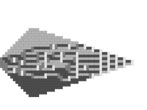
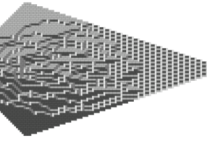
Figure 19. The domino tilings associated with random perfect matchings of the pinecone $P(n;1,3,2,2)$, for $n=26$ and then $n=70$.

The reader will quickly notice that in both of these random tilings, the randomness is not spatially distributed in a uniform manner. Near the boundary, there is a good deal of order, with tiles lined up the same way as their neighbors; only in the interior does one find random-looking behavior.

This phenomenon is not specific to pinecones, but has been observed for a wide variety of two-dimensional tiling models over the past decade, from [7] and [8] to [16]. The most-studied case is the Aztec diamond graph ($(i,j,k,\ell)=(1,1,1,1)$, in our notation); in this case, it has been shown that in a suitable asymptotic sense there is a sharp boundary between the part of the tiling that is random and the part that is orderly, and that this boundary is (asymptotically) a perfect circle. A similar sort of domain-boundary is visible in Figure 19; assuming that the theory for pinecones is analogous to the theory for Aztec diamond graphs, it would be interesting to know the asymptotic shape of the domain-boundary for $(i,j,k,\ell)$-pinecones as $n\rightarrow\infty$.

One interesting feature of Gale-Robinson pinecones is that we can write the definition in a way that makes sense even when the parameters $(i,j,k,\ell)$ cease to be integers. Formula (2) can be rewritten as

$$\begin{array}[]{lll}U(t,r,c)&=&2c+r-3-2\left\lfloor{\displaystyle\mu c+\kappa r+\iota-t}\right\rfloor,\\ \\ L(t,r,c)&=&2c+r-3-2\left\lfloor{\displaystyle\mu c+\lambda r+\iota-t}\right\rfloor.\end{array}$$ (7)

where $\iota=i/j$, $\kappa=k/j$, $\lambda=\ell/j$, $\mu=m/j=\iota+1=\kappa+\lambda$, and $t=(n+1)/j$. So there is a sense in which all the pinecones discussed in this article are part of a four parameter family, parametrized by $\iota$, $\kappa$, $\lambda$ and $t$. Of course, the graphs do not vary continuously in these variables (being discrete elements in a countable set, namely the set of all finite graphs, how could they?), but this parametrization seems likely to be natural for some purposes, e.g., the study of random perfect matchings of pinecones. (It is to be expected that a coherent limit-law with $t\rightarrow\infty$ will prevail for any fixed choice of $(\iota,\kappa,\lambda)$, whether or not $\iota$, $\kappa$, and $\lambda$ are rational.) It should be noted, incidentally, that if one chooses parameters $(i,j,k,\ell)$ with a greater common divisor $d>1$, the sequence of pinecones one gets from our construction is the same as the sequence of pinecones that one gets from the parameters $(i/d,j/d,k/d,\ell/d)$, except that each pinecone in the latter sequence is repeated $d$ times in the former sequence; this observation follows easily from the $\iota,\kappa,\lambda$ formulation of the definitions of $U(\cdot)$ and $L(\cdot)$.

5.3. Closed-form expressions

One feature common to sequences satisfying three-term or four-term Gale-Robinson recurrences is that the terms grow at quadratic exponential rate. Indeed, it is easy to verify, from the discussion of pinecones, that in the infinite sequence of graphs associated with any particular three-term Gale-Robinson recurrence, the $n$th graph has $O(n^{2})$ vertices, with each vertex having degree at most 4. It follows from this that Gale-Robinson sequences have at most exponential-quadratic growth; that is, the $n$th term is bounded above by $C^{n^{2}}$ for all sufficiently large $C$. In some cases, an exact formula is possible; we have already mentioned the “Aztec diamond case” $i=j=k=\ell=1$, and in the case $(i,j,k,\ell,m)=(6,1,4,3,7)$ there is an exact formula for $a(n)$ of the form $2^{e_{2}(n)}3^{e_{3}(n)}$ where the exponents $e_{2}(n)$ and $e_{3}(n)$ are given by quadratic polynomials in $n$ whose coefficients are periodic functions of $n$ (we thank Michael Somos for bringing this special case of the Gale-Robinson recurrence to our attention, and we raise the question of whether there are other instances of Gale-Robinson sequences being given by simple exact formulas). However, in general such algebraic formulas do not exist. Instead, one must be content with formulas that express the $n$th term in terms of Jacobi theta functions. This link with the analytic world is what motivated Michael Somos to introduce the Somos-$k$ sequences to begin with. E.g., back in 1993, Somos announced (without proof) that the $n$th term of the Somos-6 sequence is given by $f(n-2.5,n-2.5)$ where

$$f(x,y)=c_{1}c_{2}^{xy}\sum_{k_{2}=-\infty}^{\infty}(-1)^{k_{2}}\sum_{k_{1}=-\infty}^{\infty}g(k_{1},k_{2},x,y),$$

$$g(k_{1},k_{2},x,y)=c_{3}^{k_{1}^{2}}c_{4}^{k_{2}^{2}}c_{5}^{k_{1}k_{2}}\cos(c_{6}k_{1}x+c_{7}k_{2}y),$$

$$c_{1}=0.875782749065950194217251...,$$

$$c_{2}=1.084125925473763343779968...,$$

$$c_{3}=0.114986002186402203509006...,$$

$$c_{4}=0.077115634258697284328024...,$$

$$c_{5}=1.180397390176742642553759...,$$

$$c_{6}=1.508030831265086447098989...,$$

$$c_{7}=2.551548771413081602906643...$$

(See http://jamespropp.org/somos/elliptic for a similar but simpler formula for the Somos-4 sequence.) However, as far as we are aware, nobody has proposed (or even conjectured) a fully general analytic formula for the terms of sequences satisfying three-term Gale-Robinson recurrences. A more detailed discussion of the analytic properties of such sequences can be found in [15], which also gives some of the history of these sequences.

It is worth mentioning that for the Somos-4 sequence, there exists a unique constant $c$ such that $s(n)$ (the $n$th term of the sequence) is on the order of $c^{n^{2}}$, but that the behavior of $s(n)/c^{n^{2}}$ is oscillatory; see http://jamespropp.org/somos/elliptic. Let us also mention a recent paper by Xin [27] where the Somos-4 numbers are expressed as determinants of Hankel matrices with integer coefficients.

5.4. Analogy with the KP hierarchy

We conclude with some remarks (based on some unpublished remarks of Andrew Hone) about the analogy between Somos sequences and the like and the hierarchy of solutions to an integrable PDE like the KdV equation, followed by our own speculation about a direction for further study that the analogy might suggest.

The equation

$$u_{xxx}+6uu_{x}+u_{t}=0,$$

where $u=u(x,t)$ is the function we want to solve for and subscripts indicate partial differentiation (e.g., $u_{xxx}=\frac{\partial^{3}u}{\partial x^{3}}$) is known as the KdV equation, and has played a crucial role in the modern theory of partial differential equation, as part of a large family of equations with related properties (the “KP hierarchy”). If one sets $u=2(\partial_{x})^{2}\log F$ one can rewrite the PDE in the compact form

$$(D_{x}D_{x}D_{x}D_{x}+D_{x}D_{t})(F\otimes F)=0$$

where $D_{x}$ and $D_{t}$ are the “Hirota $D$-operators” acting on tensor-pairs of functions via

$$D_{x}(f(x,t)\otimes g(x,t))=(\partial_{x_{1}}-\partial_{x_{2}})f(x_{1},t)g(x_{2},t)|_{x_{1}=x_{2}=x}$$

and

$$D_{t}(f(x,t)\otimes g(x,t))=(\partial_{t_{1}}-\partial_{t_{2}})f(x,t_{1})g(x,t_{2})|_{t_{1}=t_{2}=t}.$$

(Note that in the literature on KdV, this tensor product is traditionally written as $f\cdot g$ rather than $f\otimes g$ and is called the “dot-product”, but it is a tensor product, not an inner product). More generally, the bilinear method is the trick of rewriting PDEs in the form $P(D_{x},D_{y},\ldots)(F\otimes F)=0$. Hirota operators are antisymmetric, so we can think of them as actions on the antisymmetric square of a vector space of functions. For more on the Hirota method, see e.g. [14].

Analogously, if we take $V$ to be the vector space of real- (or complex-) valued bilaterally infinite sequences $(\ldots,s_{0},\ldots)$, we may define, for every pairs of integers $i,j$, a bilinear shift operator $V\otimes V\rightarrow V$ sending $(s_{n})_{-\infty}^{\infty}\otimes(t_{n})_{-\infty}^{\infty}$ to $(s_{n+i}t_{n+j})_{-\infty}^{\infty}$ (the sequence whose $n$th term is $s_{n+i}t_{n+j}$ for all $n\in\mathbb{Z}$). These operators, graded by $i+j$, generate a graded ring of bilinear shift-operators, and the Somos sequences and Gale-Robinson sequences are special instances of sequences $(s_{n})_{-\infty}^{\infty}$ for which the tensor-square $(s_{n})_{-\infty}^{\infty}\otimes(s_{n})_{-\infty}^{\infty}$ lies in the kernel of a particular bilinear operator. It has been noticed that for a typical Somos or Gale-Robinson sequence, the tensor-square of the sequence, in addition to being annihilated by the “defining” bilinear operator, is annihilated by infinitely many others as well. In fact, there is more than just an analogy at work here: each GR recurrence can be written in terms of Hirota differential operators by taking exponentials (see [23]). Hopefully, by combining algebraic, analytic, and combinatorial tools, future researchers will shed some light on this intriguing phenomenon.

References

- [1] N. Anzalone, J. Baldwin, I. Bronshtein, and T. K. Petersen. A reciprocity theorem for monomer-dimer coverings. In Discrete models for complex systems, DMCS ’03 (Lyon), Discrete Math. Theor. Comput. Sci. Proc., AB, pages 179–193 (electronic). Assoc. Discrete Math. Theor. Comput. Sci., Nancy, 2003. Available on the arXiv at math.CO/0304359.
- [2] M. Beck and T. Zaslavsky. Inside-out polytopes. Adv. Math., 205(1):134–162, 2006.
- [3] A. T. Benjamin and J. J. Quinn. Proofs that really count: The art of combinatorial proof, volume 27 of The Dolciani Mathematical Expositions. Mathematical Association of America, Washington, DC, 2003.
- [4] J. Berstel and C. Reutenauer. Another proof of Soittola’s theorem. Theoret. Comput. Sci., 393(1-3):196–203, 2008.
- [5] D. Bressoud and J. Propp. How the alternating sign matrix conjecture was solved. Notices Amer. Math. Soc., 46(6):637–646, 1999.
- [6] G. Carroll and D. Speyer. The cube recurrence. Electron. J. Combinat., 11(1)(article R73), 2004.
- [7] H. Cohn, N. Elkies, and J. Propp. Local statistics for random domino tilings of the Aztec diamond. Duke Math. J., 85(1):117–166, 1996.
- [8] H. Cohn, M. Larsen, and J. Propp. The shape of a typical boxed plane partition. New York J. Math., 4:137–165 (electronic), 1998.
- [9] P. Di Francesco and R. Kedem. Q-systems, heaps, paths and cluster positivity. Available on the arXiv at arXiv:0811.3027.
- [10] N. Elkies, G. Kuperberg, M. Larsen, and J. Propp. Alternating-sign matrices and domino tilings. I. J. Algebraic Combin., 1(2):111–132, 1992.
- [11] S. Fomin and A. Zelevinsky. The Laurent phenomenon. Adv. in Appl. Math., 28(2):119–144, 2002.
- [12] D. Gale. Somos sequence update. Math. Intelligencer, 13(4):49–50, 1991.
- [13] D. Gale. The strange and surprising saga of the Somos sequences. Math. Intelligencer, 13(1):40–42, 1991.
- [14] R. Hirota. The direct method in soliton theory. Cambridge University Press, San Diego, CA, 2004. Cambridge Tracts in Mathematics, No. 155.
- [15] A. N. W. Hone. Discrete dynamics, integrability and integer sequences. Imperial College Press, in preparation.
- [16] R. Kenyon, A. Okounkov, and S. Sheffield. Dimers and amoebae. Ann. of Math. (2), 163(3):1019–1056, 2006. Available on the arXiv at math-ph/0311005.
- [17] E. H. Kuo. Applications of graphical condensation for enumerating matchings and tilings. Theoret. Comput. Sci., 319(1-3):29–57, 2004. Available on the arXiv at math.CO/0304090.
- [18] J. Propp. The combinatorics of frieze patterns and Markoff numbers. Available on the arXiv at math.CO/0511633.
- [19] J. Propp. A reciprocity theorem for domino tilings. Electron. J. Combin., 8(1):Research Paper 18, 9 pp. (electronic), 2001. Available on the arXiv at math.CO/0104011.
- [20] J. Propp and D. Wilson. Coupling from the past: a user’s guide. In Microsurveys in discrete probability (Princeton, NJ, 1997), volume 41 of DIMACS Ser. Discrete Math. Theoret. Comput. Sci., pages 181–192. Amer. Math. Soc., Providence, RI, 1998.
- [21] J. G. Propp and D. B. Wilson. Exact sampling with coupled Markov chains and applications to statistical mechanics. Random Structures Algorithms, 9(1-2):223–252, 1996.
- [22] D. P. Robbins and H. Rumsey, Jr. Determinants and alternating sign matrices. Adv. in Math., 62(2):169–184, 1986.
- [23] N. Saitoh and S. Saito. General solutions to the Bäcklund transformation of Hirota’s bilinear difference equation. J. Phys. Soc. Japan, 56(5):1664–1674, 1987.
- [24] N. J. A. Sloane and S. Plouffe. The encyclopedia of integer sequences. Academic Press Inc., San Diego, CA, 1995. http://www.research.att.com/njas/sequences/index.html.
- [25] D. E. Speyer. Perfect matchings and the octahedron recurrence. J. Algebraic Combin., 25(3):309–348, 2007. Available on the arXiv at math.CO/0402452.
- [26] R. P. Stanley. Enumerative combinatorics. Vol. 1, volume 49 of Cambridge Studies in Advanced Mathematics. Cambridge University Press, Cambridge, 1997.
- [27] G. Xin. Proof of the Somos-4 Hankel determinants conjecture. Adv. in Appl. Math., 42(2):152–156, 2009.
- [28] A. Zabrodin. A survey of Hirota’s difference equations. Available on the arXiv at solv-int/9704001.