Beurling’s free boundary value problem
in conformal geometry

Florian Bauer, Daniela Kraus, Oliver Roth and Elias Wegert

January 10, 2009

Abstract. The subject of this paper is Beurling’s celebrated extension of the Riemann mapping theorem [5]. Our point of departure is the observation that the only known proof of the Beurling–Riemann mapping theorem contains a number of gaps which seem inherent in Beurling’s geometric and approximative approach. We provide a complete proof of the Beurling–Riemann mapping theorem by combining Beurling’s geometric method with a number of new analytic tools, notably $H^{p}$–space techniques and methods from the theory of Riemann–Hilbert–Poincaré problems. One additional advantage of this approach is that it leads to an extension of the Beurling–Riemann mapping theorem for analytic maps with prescribed branching. Moreover, it allows a complete description of the boundary regularity of solutions in the (generalized) Beurling–Riemann mapping theorem extending earlier results that have been obtained by PDE techniques. We finally consider the question of uniqueness in the extended Beurling–Riemann mapping theorem.

1 Introduction

Let $\mathcal{H}_{0}({\mathbb{D}})$ denote the set of analytic functions $f$ on the unit disk ${\mathbb{D}}:=\{z\in{\mathbb{C}}\,:\,|z|<1\}$ normalized by $f(0)=0<f^{\prime}(0)$ and let $\Phi:{\mathbb{C}}\to{\mathbb{R}}$ be a continuous, positive and bounded function. Beurling’s conformal geometric free boundary value problem [5] asks for univalent functions $f\in{\cal H}_{0}({\mathbb{D}})$ that satisfy

$$\lim\limits_{z\to\xi}\left(|f^{\prime}(z)|-\Phi(f(z))\right)=0\,,\qquad\xi\in\partial{\mathbb{D}}.$$ (1.1)

We call any $f\in\mathcal{H}_{0}({\mathbb{D}})$ (univalent or not) for which (1.1) holds a solution for $\Phi$.

Beurling’s paper [5] and its successor [6] proved to be quite influential in various different branches of mathematics such as partial differential equations, geometric function theory and Riemann–Hilbert problems. For instance, some of Beurling’s ideas are nowadays extensively used in the theory of free boundary value problems for PDEs and in fact the papers [5, 6] are widely considered as some of the pioneering papers on free boundary value problems (see [14, 16]). They also found considerable attention in geometric complex analysis and conformal geometry, see for instance [1, 3, 4, 10, 11, 17, 22] as some of the more recent references.

One of the purposes of the present paper is to provide a thorough and complete discussion of Beurling’s original free boundary value problem (1.1). This requires advanced analytic tools from $H^{p}$–space theory and Riemann–Hilbert–Poincaré problems, which have not been used for this purpose before. These tools make it possible to establish in addition a number of extensions of Beurling’s results e.g. to solutions with prescribed critical points, to describe the boundary behaviour of the solutions and to deduce new sufficient conditions for uniqueness of solutions.

Beurling’s treatment of the boundary value problem (1.1) in [5] is based on an ingenious geometric version of Perron’s method from the theory of subharmonic functions. He defines a class of supersolutions and subsolutions for $\Phi$ (see below for the precise definition) and shows that there is always a “largest” univalent subsolution $f^{*}$ and a “smallest” univalent supersolution $g^{*}$. He then asserts that both $f^{*}$ and $g^{*}$ are in fact solutions for $\Phi$, but his arguments are in both cases incomplete. For instance, Beurling’s approach to prove that $g^{*}$ is a solution for $\Phi$ is in two steps. First he deals with the special case that $g^{*}({\mathbb{D}})$ is of “Schoenfliess type”. In order to handle the general case, he then makes use of the assertion that every strictly shrinking sequence of (normalized) simply connected domains converges in the sense of kernel convergence to a domain of Schoenfliess type. This, however, is not true in general (see Appendix 2 below for an explicit counterexample), so Beurling’s method is destined to fail here. In order to circumvent this difficulty we combine Beurling’s geometric approach with more advanced analytic tools. As a result, we obtain an efficient method that avoids “domains of Schoenfliess type” altogether and allows a treatment of the smallest univalent supersolution without unnecessary approximation techniques.

We also establish the existence of nonunivalent solutions for $\Phi$ with prescribed branch points. There are a number of reasons for taking nonunivalent solutions into account. For instance, it seems indispensable to find first nonunivalent solutions in order to prove that there are always univalent solutions. The proof of existence of nonunivalent solutions in this paper is based on a fixed–point argument and closes another possible gap in Beurling’s original approach, see Section 4.1. A second reason for allowing nonunivalent solutions is that Beurling’s problem might be viewed as a special case of a certain type of generalized Riemann–Hilbert problems (sometimes called Riemann–Hilbert–Poincaré problems). These problems deal with the construction of analytic maps with prescribed boundary behaviour and preassigned branch points. We note that in this context a variant of Beurling’s boundary value problem with specified critical points played a key role in recent work on “hyperbolic” Blaschke products (see [10]) and on infinite Blaschke products with infinitely many critical points (see [19]).

Finally, we discuss in detail the boundary behaviour of the solutions for $\Phi$. For univalent solutions Beurling’s problem (1.1) might be viewed as a free boundary value problem for $\Omega=f(\mathbb{D})$ involving PDEs (see Appendix 1), but this relation breaks down for nonunivalent solutions. Thus one can apply techniques from PDEs to study the boundary regularity of univalent solutions, but not for nonunivalent solutions. In particular, it follows from results of Alt & Caffarelli [2], Kinderlehrer & Nirenberg [18] and Gustafsson & Shahgholian [14] that every univalent solution $f$ for $\Phi$ is of class $C^{1,\alpha}(\partial{\mathbb{D}})$ for some $0<\alpha<1$ when $\Phi$ is Hölder continuous, that $f\in C^{k+1,\alpha}(\partial{\mathbb{D}})$ when $\Phi\in C^{k,\alpha}$, $k\geq 1$ and $0<\alpha<1$, and that $f$ is real analytic across $\partial{\mathbb{D}}$ when $\Phi$ is real analytic (see also Sakai [23, 24]). The result for real analytic $\Phi$ has recently been extended to all (i.e. not necessarily univalent) solutions in [22] using a completely different approach. Based on a method specific to Beurling’s problem, we complement the results of [2, 18, 14] in Theorem 4.4 below by showing that every solution for $\Phi$ belongs to $C^{k+1,\alpha}(\partial{\mathbb{D}})$ provided $\Phi$ is of class $C^{k,\alpha}$ for $0<\alpha<1$ and all $k\geq 0$.

This paper is organized as follows. We start in Section 2 with a discussion of the set $A_{\Phi}$ of subsolutions to Beurling’s boundary value problem (1.1) including a number of simplifications and generalizations of Beurling’s original treatment of $A_{\Phi}$. In Section 3 we show that the set $B_{\Phi}$ of univalent supersolutions can be handled almost identically as the set $A_{\Phi}$ using the (usual) topology of locally uniform convergence on the unit disk. In order to incorporate the boundary behaviour of univalent supersolutions we continuously embed $B_{\Phi}$ in the Hardy space $H^{p}$, $0<p<1/2$. This is possible by results of Feng and MacGregor [9] on the integral means of the derivative of univalent functions and Hardy–Littlewood–type arguments. In this context, the key result is Lemma 3.4 below. Section 4 is divided into four parts. In §4.1 we consider a class of Riemann–Hilbert–Poincaré problems, which includes Beurling’s free boundary value problem as special case. We first establish a representation formula for solutions to this more general type of boundary value problem. The existence of such solutions is then proved by an application of Schauder’s fixed point principle. The representation formula also leads to a full description of the boundary behaviour of solutions in §4.2. Armed with at least nonunivalent solutions we then return to Beurling’s original boundary problem in §4.3 and §4.4. In §4.3 we will see that the maximal subsolution is in fact a (univalent) solution. Here we make essential use of the results of §4.1. The proof that the minimal univalent supersolution is a solution is much more elaborate and is given in §4.4. In Section 5 we briefly discuss the question of uniqueness in Beurling’s boundary value problem and find (slight) generalizations of uniqueness results due to Beurling [5] and Gustafsson & Shahgholian [14] (see also [17]). We conclude the paper with two appendices. Appendix 1 indicates how Beurling’s problem for univalent functions is connected with a class of free boundary value problems for PDEs, which also arise in many areas of physics (Hele–Shaw flows) as well as in mathematical analysis (Quadrature domains). Finally, in Appendix 2 we discuss an explicit counterexample to Beurling’s method of proof in [5].

2 Subsolutions

In the sequel we denote the Poisson kernel on ${\mathbb{D}}$ by

$$P(z,e^{it}):=\mathop{{\rm Re}}\left(\frac{e^{it}+z}{e^{it}-z}\right)\,,\qquad z\in{\mathbb{D}}\,,\,\,t\in{\mathbb{R}}\,,$$

and use the notation

$$||\varphi||:=\sup\limits_{w\in{\mathbb{C}}}|\varphi(w)|$$

for any bounded function $\varphi:{\mathbb{C}}\to{\mathbb{C}}$.

Definition 2.1

Let $\Phi:{\mathbb{C}}\to{\mathbb{R}}$ be a positive, continuous and bounded function. The set $A_{\Phi}$ is defined by

$$A_{\Phi}:=\left\{f\in{\cal H}_{0}({\mathbb{D}})\,:\,\limsup_{|z|\to 1}\left(|f^{\prime}(z)|-\Phi(f(z))\right)\leq 0\right\}\,.$$

We call every function $f\in A_{\Phi}$ a subsolution for $\Phi$.

The goal of this section is to show that there is always a unique “largest” subsolution $f^{*}$ for $\Phi$ and that this largest subsolution is univalent:

Theorem 2.2

Let $\Phi:{\mathbb{C}}\to{\mathbb{R}}$ be a positive, continuous and bounded function. Then there exists a unique function $f^{*}\in A_{\Phi}$ such that

$$f^{*\,\prime}(0)=\sup\limits_{f\in A_{\Phi}}f^{\prime}(0)\,.$$

The function $f^{*}$ is univalent in ${\mathbb{D}}$ with $f^{*}({\mathbb{D}})=A^{*}$, where

$$A^{*}:=\bigcup\limits_{f\in A_{\Phi}}f({\mathbb{D}})\,.$$

In particular, $f({\mathbb{D}})\subseteq A^{*}$ for all $f\in A_{\Phi}$.

We call the function $f^{*}$ of Theorem 2.2 the maximal univalent subsolution for $\Phi$. The following simple facts about subsolutions will be used in the proof of Theorem 2.2.

Lemma 2.3

Let $\Phi:{\mathbb{C}}\to{\mathbb{R}}$ be a positive, continuous and bounded function.

• Any subsolution for $\Phi$ has a (Lipschitz) continuous extension to the closed unit disk $\overline{{\mathbb{D}}}$. The set $A_{\Phi}$ is uniformly bounded on $\overline{{\mathbb{D}}}$ and equicontinuous at every point $z_{0}\in\overline{{\mathbb{D}}}$.

• A function $f\in\mathcal{H}_{0}({\mathbb{D}})$ with a continuous extension to $\overline{{\mathbb{D}}}$ is a subsolution for $\Phi$ if and only if

  $$\log|f^{\prime}(z)|\leq\frac{1}{2\pi}\int\limits_{0}^{2\pi}P(z,e^{it})\,\log\Phi(f(e^{it}))\,dt\,,\qquad z\in{\mathbb{D}}\,.$$ (2.1)

• If a sequence of subsolutions for $\Phi$ converges locally uniformly in ${\mathbb{D}}$, then the limit function $f$ is either again a subsolution for $\Phi$ or $f\equiv 0$.

• Let $f\in A_{\Phi}$ and let $\Psi:{\mathbb{C}}\to{\mathbb{R}}$ be a positive, continuous and bounded function with $\Psi>\Phi$. Then for all $r<1$ sufficiently close to $1$ the function $f_{r}(z):=f(rz)$ is a subsolution for $A_{\Psi}$.

Remark 2.4

Lemma 2.3 shows that for treating the class $A_{\Phi}$ one can use the uniform topology on the closed unit disk $\overline{{\mathbb{D}}}$. This facilitates the handling of subsolutions. Beurling proved Lemma 2.3 (b) and (c) for univalent subsolutions. We need the general case.

Proof. (a)  The maximum principle implies that for any $f\in A_{\Phi}$ the function $|f^{\prime}|$ is bounded above in ${\mathbb{D}}$ by $M:=||\Phi||$, so $f$ has a (Lipschitz) continuous extension to $\overline{{\mathbb{D}}}$. Note that the Lipschitz constant is independent of $f$, so $A_{\Phi}$ is uniformly bounded and equicontinuous in $\overline{{\mathbb{D}}}$.

(b)   This follows from the fact that the Poisson integral on the righthand side of (2.1) is harmonic in ${\mathbb{D}}$ with boundary values $\log\Phi(f(\xi))$, $|\xi|=1$.

(c)   Let $f_{n}\in A_{\Phi}$ and suppose that $(f_{n})_{n}$ converges locally uniformly to a holomorphic function $f:{\mathbb{D}}\to{\mathbb{C}}$ with $f(0)=0$. Then by (a) and the Arzelà–Ascoli theorem a subsequence $(f_{n_{k}})_{k}$ converges uniformly on $\overline{{\mathbb{D}}}$, so $f:\overline{{\mathbb{D}}}\to{\mathbb{C}}$ is continuous. If $f\not\equiv 0$, then $f$ is not constant. Hence $\log|f^{\prime}(z)|$ is a subharmonic function on ${\mathbb{D}}$ and part (b) shows that $f\in A_{\Phi}$ because

$$\log|f^{\prime}(z)| = \lim\limits_{k\to\infty}\log|f_{n_{k}}^{\prime}(z)|\leq\lim\limits_{k\to\infty}\frac{1}{2\pi}\int\limits_{0}^{2\pi}P(z,e^{it})\,\log\Phi(f_{n_{k}}(e^{it}))\,dt$$

$$= \frac{1}{2\pi}\int\limits_{0}^{2\pi}P(z,e^{it})\,\log\Phi(f(e^{it}))\,dt\,,\qquad z\in{\mathbb{D}}\,.$$

(d)   Assume to the contrary that $f_{r_{n}}\not\in A_{\Psi}$ for some sequence of radii $r_{n}\nearrow 1$. Then there are points $|\xi_{n}|=1$ such that $r_{n}|f^{\prime}(r_{n}\xi_{n})|=|f^{\prime}_{r_{n}}(\xi_{n})|>\Psi(f_{r_{n}}(\xi_{n}))=\Psi(f(r_{n}\xi_{n}))\,.$ We may assume $r_{n}\xi_{n}\to\xi\in\partial{\mathbb{D}}$. Then

$$\limsup_{z\to\xi}|f^{\prime}(z)|\geq\limsup_{n\to\infty}|f^{\prime}(r_{n}\xi_{n})|\geq\Psi(f(\xi))>\Phi(f(\xi))\,,$$

which contradicts $f\in A_{\Phi}$. $\blacksquare$

The main tool needed for the proof of Theorem 2.2 is a geometric version of the Poisson modification of a subharmonic function. For this Beurling introduced an “extended” union of domains in the complex plane which is always simply connected.

Definition 2.5 (Extended union)

Let $D_{1}$ and $D_{2}$ be two bounded domains in ${\mathbb{C}}$ with $0\in D_{1}\cap D_{2}$. We call the complement of the unbounded component of $\hat{{\mathbb{C}}}\backslash(D_{1}\cup D_{2})$ the extended union of $D_{1}$ and $D_{2}$ and denote it by ${\rm EU}(D_{1},D_{2})$.

Beurling has a formally different, but equivalent definition for ${\rm EU}(D_{1},D_{2})$. We note the following easily verified properties of the extended union.

• (EU1)   ${\rm EU}(D_{1},D_{2})$ is the smallest simply connected domain which contains $D_{1}\cup D_{2}$.

• (EU2)   If $D_{1}\subseteq D_{1}^{\prime}$ and $D_{2}\subseteq D_{2}^{\prime}$, then ${\rm EU}(D_{1},D_{2})\subseteq{\rm EU}(D_{1}^{\prime},D_{2}^{\prime})$.

• (EU3)   $\partial{\rm EU}(D_{1},D_{2})\subseteq\partial D_{1}\cup\partial D_{2}$.

Definition 2.6 (Upper Beurling modification)

Let $f_{1},f_{2}\in\mathcal{H}_{0}({\mathbb{D}})$. Then the conformal map $f$ from ${\mathbb{D}}$ onto ${\rm EU}(f_{1}({\mathbb{D}}),f_{2}({\mathbb{D}}))$ normalized by $f(0)=0$ and $f^{\prime}(0)>0$ is called the upper Beurling modification of $f_{1}$ and $f_{2}$.

Lemma 2.7

Let $\Phi:{\mathbb{C}}\to{\mathbb{R}}$ be a positive, continuous and bounded function and $f_{1},f_{2}$ two subsolutions for $\Phi$. Then the upper Beurling modification of $f_{1}$ and $f_{2}$ is also a subsolution for $\Phi$.

The following proof is different from Beurling’s proof insofar as we replace Beurling’s Riemann surface construction by a simple application of the Julia–Wolff lemma (see [21, p. 82]).

Proof. (i)   We first prove the lemma under the additional assumption that $f_{1}$ and $f_{2}$ are analytic on $\overline{{\mathbb{D}}}$. In this case the boundary of the extended union $D:={\rm EU}(f_{1}({\mathbb{D}}),f_{2}({\mathbb{D}}))$ is locally connected and consists of finitely many analytic Jordan arcs. Thus the upper Beurling modification $f$ of $f_{1}$ and $f_{2}$ has an analytic continuation across $\partial{\mathbb{D}}\backslash N$, where $N\subset\partial{\mathbb{D}}$ is a finite set, and $D$ is a Smirnov domain [21, p. 60 & p. 163], i.e., $f$ satisfies

$$\log|f^{\prime}(z)|=\frac{1}{2\pi}\int\limits_{0}^{2\pi}P(z,e^{it})\,\log|f^{\prime}(e^{it})|\,dt\,,\qquad z\in{\mathbb{D}}\,.$$ (2.2)

Since $\partial D\subset f_{1}(\partial{\mathbb{D}})\cup f_{2}(\partial{\mathbb{D}})$, there is in particular for every $\xi\in\partial{\mathbb{D}}\backslash N$ a point $\xi_{0}\in\partial{\mathbb{D}}$ such that $f(\xi)=f_{1}(\xi_{0})$ or $f(\xi)=f_{2}(\xi_{0})$. If $f(\xi)=f_{1}(\xi_{0})$, then the function $w(z):=f^{-1}(f_{1}(z))$ maps ${\mathbb{D}}$ into ${\mathbb{D}}$ with $w(0)=0$ and $w(\xi_{0})=\xi$. By the Julia–Wolff lemma $|w^{\prime}(\xi_{0})|\geq 1$, so

$$|f^{\prime}(\xi)|=\frac{|f_{1}^{\prime}(\xi_{0})|}{|w^{\prime}(\xi_{0})|}\leq|f_{1}^{\prime}(\xi_{0})|\leq\Phi(f_{1}(\xi_{0}))=\Phi(f(\xi))\,.$$ (2.3)

The same conclusion holds if $f(\xi)=f_{2}(\xi_{0})$. Thus (2.3) holds for every $\xi\in\partial{\mathbb{D}}$ except for finitely many points. Therefore (2.2) leads to

$$\log|f^{\prime}(z)|\leq\frac{1}{2\pi}\int\limits_{0}^{2\pi}P(z,e^{it})\,\log\Phi(f(e^{it}))\,dt\,,\qquad z\in{\mathbb{D}}\,.$$

This shows $f\in A_{\Phi}$.

(ii)   We now turn to the general case. Let $\Psi:{\mathbb{C}}\to{\mathbb{R}}$ be a positive, continuous and bounded function with $\Psi>\Phi$. In view of Lemma 2.3 (d), the functions $f_{1}(rz)$ and $f_{2}(rz)$ belong to $A_{\Psi}$ for all $0<r_{0}<r<1$. By what we have shown above, the upper Beurling modification $f_{r}$ of $f_{1}(rz)$ and $f_{2}(rz)$ belongs to $A_{\Psi}$ for every $0<r_{0}<r<1$. Now $f_{r}$ maps ${\mathbb{D}}$ conformally onto $D_{r}:={\rm EU}(f_{1}(r{\mathbb{D}}),f_{2}(r{\mathbb{D}}))$. Note that $D_{r}\subseteq D_{r^{\prime}}$ whenever $0<r<r^{\prime}<1$ in view of (EU2). Thus as $r\to 1$ the domains $D_{r}$ converge in the sense of kernel convergence to the simply connected domain

$$D^{\prime}:=\bigcup\limits_{r_{0}<r<1}D_{r}\,$$

with $f_{1}({\mathbb{D}})\cup f_{2}({\mathbb{D}})\subset D^{\prime}$. This implies $D\subset D^{\prime}$ by (EU1). On the other hand, by (EU2), we have $D_{r}\subseteq D$, so $D^{\prime}\subseteq D$. Carathéodory’s convergence theorem shows $f_{r}\to f$ locally uniformly in ${\mathbb{D}}$, see [21, Chap. 1.4]. Since $f_{r}\in A_{\Psi}$ for all $r$ close enough to $1$, Lemma 2.3 (c) gives $f\in A_{\Psi}$. As $\Psi$ is an arbitrary positive, continuous and bounded function on ${\mathbb{D}}$ with $\Psi>\Phi$, we conclude $f\in A_{\Phi}$. $\blacksquare$

Remark 2.8

The approximation argument in the above proof cannot be avoided entirely. This is due to the fact that subsolutions even though they are Lipschitz continuous up to the unit circle may have a very bad behaved derivative. For instance the well–known example of Duren, Shapiro and Shields [8] (see also [21, p. 159]) of a conformal map $f$ not of Smirnov type satisfies $|f^{\prime}|<1$ in ${\mathbb{D}}$, so belongs to $A_{\Phi}$ for $\Phi\equiv 1$. Even for a solution $f$ for $\Phi$ the derivative $f^{\prime}$ does not need to have a continuous extension to $\overline{{\mathbb{D}}}$, see Example 4.6.

Proof of Theorem 2.2. By Lemma 2.3 there is a function $f^{*}\in A_{\Phi}$ such that

$$f^{*\,\prime}(0)=\max\limits_{f\in A_{\Phi}}f^{\prime}(0)\,.$$

We need to prove that $f^{*}$ is univalent and $f({\mathbb{D}})\subseteq f^{*}({\mathbb{D}})$ for every $f\in A_{\Phi}$. Let $f\in A_{\Phi}$ and let $F$ be the upper Beurling modification of $f$ and $f^{*}$. Lemma 2.7 shows $F\in A_{\Phi}$, so $F^{\prime}(0)\leq f^{*\,\prime}(0)$. On the other hand, we have $F({\mathbb{D}})={\rm EU}(f^{*}({\mathbb{D}}),f({\mathbb{D}}))\supseteq f^{*}({\mathbb{D}})$. By the principle of subordination this implies $F=f^{*}$. Hence $f^{*}$ is univalent and $f({\mathbb{D}})\subseteq f^{*}({\mathbb{D}})$. Now it is also clear that $f^{*}$ is uniquely determined. $\blacksquare$

3 Univalent supersolutions

Definition 3.1

Let $\Phi:{\mathbb{C}}\to{\mathbb{R}}$ be a positive, continuous and bounded function. Then the set $B_{\Phi}$ is defined by

$$B_{\Phi}:=\left\{g\in{\cal H}_{0}({\mathbb{D}})\,:\,g\text{ univalent and }\liminf_{|z|\to 1}\left(|g^{\prime}(z)|-\Phi(g(z))\right)\geq 0\right\}\,.$$

We call any function $g\in B_{\Phi}$ a univalent supersolution for $\Phi$.

Note that we consider only univalent supersolutions, see Remark 5.5 for a partial explanation. We establish in this paragraph the following counterpart to Theorem 2.2.

Theorem 3.2

Let $\Phi:{\mathbb{C}}\to{\mathbb{R}}$ be a positive, continuous and bounded function. Then there exists a unique function $g^{*}\in B_{\Phi}$ such that

$$g^{*\,\prime}(0)=\inf\limits_{g\in B_{\Phi}}g^{\prime}(0)\,.$$

The function $g^{*}$ maps ${\mathbb{D}}$ conformally onto $B^{*}$, where

$$B^{*}:=\bigcap\limits_{g\in B_{\Phi}}g({\mathbb{D}})\,.$$

In particular, $B^{*}\subseteq g({\mathbb{D}})$ for all $g\in B_{\Phi}$.

We call the function $g^{*}$ of Theorem 3.2 the minimal univalent supersolution for $\Phi$.

Supersolutions are considerably more complicated than subsolutions since they do not need to be continuous up to the unit circle. In particular, the topology of uniform convergence on the closed unit disk is inappropriate for the class $B_{\Phi}$. Nevertheless, $B_{\Phi}$ can be handled in a similar way as the class $A_{\Phi}$, but now using the notion of locally uniform convergence in ${\mathbb{D}}$. For treating Beurling’s boundary value problem we ultimately need to pass from inside the unit disk to the unit circle.

Lemma 3.3

Let $\Phi:{\mathbb{C}}\to{\mathbb{R}}$ be a positive, continuous and bounded function.

• Any univalent supersolution $g$ for $\Phi$ has radial limits almost everywhere, i.e. the limit

  $$g(e^{it})=\lim\limits_{r\to 1}g(re^{it})\,,$$

  exists for a.e. $e^{it}\in\partial{\mathbb{D}}$. The boundary function $g$ belongs to $L^{p}(\partial{\mathbb{D}})$ for every $0<p<1/2$. If $g$ is bounded, then $g^{-1}$ has a continuous extension to the closure of $g({\mathbb{D}})$.

• A bounded and univalent function $g\in{\cal H}_{0}({\mathbb{D}})$ belongs to $B_{\Phi}$ if and only if

  $$\log|g^{\prime}(z)|\geq\frac{1}{2\pi}\int_{0}^{2\pi}P(z,e^{it})\log\Phi(g(e^{it}))\,dt\,,\qquad z\in{\mathbb{D}}\,.$$ (3.1)

• If a uniformly bounded sequence of univalent supersolutions for $\Phi$ converges locally uniformly in ${\mathbb{D}}$, then the limit function $g$ is again a univalent supersolution for $\Phi$.

• Let $\Psi:{\mathbb{C}}\to{\mathbb{R}}$ be a positive, continuous and bounded function with $\Psi<\Phi$ and let $g$ be a univalent supersolution for $\Phi$. If $g$ is bounded, then for all $r<1$ sufficiently close to $1$ the function $g_{r}(z):=g(rz)$ is a univalent supersolution for $\Psi$.

Proof of Lemma 3.3 (a) $\&$ (b) $\&$ (d):

(a)  A univalent holomorphic function in ${\mathbb{D}}$ belongs to the Hardy spaces $H^{p}$ for $0<p<1/2$ and has therefore radial limits almost everywhere, see [7]. If $g$ is bounded, then

$$|g^{\prime}(z)|\geq c:=\inf_{|w|\leq||g||}\Phi(w)>0\,,$$

so $|(g^{-1})^{\prime}(w)|\leq 1/c$ in $g({\mathbb{D}})$, i.e. $g^{-1}$ has a continuous extension to the closure of $g({\mathbb{D}})$.

(b)  First note that if $g\in{\cal H}_{0}({\mathbb{D}})$ is a bounded and univalent function, then, since $g({\mathbb{D}})$ is simply connected, there is a unique solution $U_{g}$ to the Dirichlet problem

$$\begin{array}[]{rclcr}\Delta u&\equiv&0&\text{in}&g({\mathbb{D}})\,\phantom{.}\\[2.84526pt] u&=&\log\Phi&\text{on}&\partial g({\mathbb{D}})\,.\end{array}$$

The function $U_{g}\circ g$ is harmonic in ${\mathbb{D}}$ and in view of part (a) has the radial limit

$$(U_{g}\circ g)(e^{it})=\log\Phi(g(e^{it}))\quad$$

for a.e. $e^{it}\in\partial{\mathbb{D}}$. Hence we can write

$$(U_{g}\circ g)(z)=\frac{1}{2\pi}\int_{0}^{2\pi}P(z,e^{it})\log\Phi(g(e^{it}))\,dt\,,\quad z\in{\mathbb{D}}\,.$$ (3.2)

Now let $g\in{\cal H}_{0}({\mathbb{D}})$ be univalent and bounded. Then $g\in B_{\Phi}$ if and only if

$$\liminf_{|z|\to 1}\left(\log|g^{\prime}(z)|-\log\Phi(g(z))\right)\geq 0\,.$$

By the univalence of $g$ we conclude that the latter inequality is equivalent to

$$\liminf_{|z|\to 1}\left(\log|g^{\prime}(z)|-U_{g}(g(z))\right)\geq 0\,.$$

The minimum principle of harmonic functions implies now that this is the same as

$$\log|g^{\prime}(z)|-U_{g}(g(z))\geq 0\,,\quad z\in{\mathbb{D}}\,.$$

Thus, by equation (3.2), $g\in B_{\Phi}$ if and only if (3.1) holds.

(d) The proof is similar to the proof of Lemma 2.3 (d) taking into account that $g$ is bounded and that we may assume that $g(r_{n}\zeta_{n})\to\eta\in\partial g({\mathbb{D}})$. The details are therefore omitted. $\blacksquare$

Part (c) of Lemma 3.3 is much more difficult to prove. Its statement is essentially due to Beurling [5], but he does not provide a proof. We first show that a locally uniformly convergent sequence of univalent holomorphic functions converges in a weak sense also on the boundary.

Lemma 3.4

Let $(f_{n})_{n}\subset{\cal{H}}_{0}({\mathbb{D}})$ be a sequence of univalent functions. Then for any $0<p<1/2$ and any $f\in H^{p}$ the following are equivalent:

• $(f_{n})_{n}$ converges to $f$ locally uniformly in ${\mathbb{D}}$.

• $\displaystyle\lim\limits_{n\to\infty}\int\limits_{0}^{2\pi}|f_{n}(e^{it})-f(e^{it})|^{p}\,dt=0$.

Lemma 3.4 implies that the class ${\cal S}=\{f\in{\cal H}_{0}({\mathbb{D}}):f\text{ univalent and }f^{\prime}(0)=1\}$ is compactly contained in $H^{p}$ for any $0<p<1/2$.

Proof. The statement (ii) $\Rightarrow$ (i) follows directly from the estimate

$$|f(z)|\leq 2^{1/p}\left(\frac{1}{2\pi}\int_{0}^{2\pi}|f(e^{it})|^{p}\,dt\right)^{1/p}\,(1-|z|)^{-1/p}\,,\quad z\in{\mathbb{D}},$$

which holds for any $f\in H^{p}$, $0<p<\infty$ ; see [7, p. 36].

To prove the implication (i) $\Rightarrow$ (ii) we follow the proof of Theorem 5 in [15]. Fix $0<\rho<1$ and choose $r$ such that $\rho<r<1$. Then

$$\begin{split}&\int\limits_{0}^{2\pi}|f_{n}(re^{it})-f(re^{it})|^{p}\,dt\\[5.69054pt] &\qquad\leq\int\limits_{0}^{2\pi}|f_{n}(re^{it})-f_{n}(\rho e^{it})|^{p}\,dt+\int\limits_{0}^{2\pi}|f_{n}(\rho e^{it})-f(\rho e^{it})|^{p}\,dt+\int\limits_{0}^{2\pi}|f(re^{it})-f(\rho e^{it})|^{p}\,dt\,.\end{split}$$

The first and the third integral have the same structure and can therefore be handled simultaneously. We may assume that $f$ is univalent, because otherwise the third integral vanishes. Let $r_{k}=r(1-1/2^{k})$ and let $N$ be the uniquely determined integer with $r_{N}\leq\rho<r_{N+1}$. Denote by $\varphi$ one of the functions $f_{n}$, $n=1,2,\ldots$, or $f$. Then, by Hardy–Littlewood (see [7, Thm. 1.9]),

$$\int\limits_{0}^{2\pi}|\varphi(re^{it})-\varphi(\rho e^{it})|^{p}\,dt \leq \int\limits_{0}^{2\pi}\left(\,\,\int\limits_{r_{N}}^{r}|\varphi^{\prime}(xe^{it})|\,dx\right)^{p}dt\leq\sum_{k=N}^{\infty}\int\limits_{0}^{2\pi}\left(\int\limits_{r_{k}}^{r_{k+1}}|\varphi^{\prime}(xe^{it})|\,dx\right)^{p}dt$$

$$\leq \sum_{k=N}^{\infty}(r_{k+1}-r_{k})^{p}\int_{0}^{2\pi}\left(\max_{r_{k}\leq x\leq r_{k+1}}|\varphi^{\prime}(xe^{it})|\right)^{p}\,dt$$

$$\leq C_{p}\,\varphi^{\prime}(0)^{p}\,\sum_{k=N}^{\infty}(r_{k+1}-r_{k})^{p}\int_{0}^{2\pi}\left|\frac{\varphi^{\prime}(r_{k+1}e^{it})}{\varphi^{\prime}(0)}\right|^{p}\,dt$$

for some constant $C_{p}$ depending only on $p$. If we assume for a moment that $p>2/5$ then for every positive integer $k$

$$\int_{0}^{2\pi}\left|\frac{\varphi^{\prime}(r_{k+1}e^{it})}{\varphi^{\prime}(0)}\right|^{p}\,dt\leq\frac{D_{p}}{(1-r_{k+1})^{3p-1}}\,,$$

where $D_{p}$ is some constant depending only on $p$, see Theorem 1 in [9]. Combining these results and using

$$S_{p}:=C_{p}D_{p}\sup_{n}f_{n}^{\prime}(0)^{p}$$

leads to

$$\int\limits_{0}^{2\pi}|\varphi(re^{it})-\varphi(\rho e^{it})|^{p}\,dt \leq S_{p}\sum_{k=N}^{\infty}\frac{(r_{k+1}-r_{k})^{p}}{(1-r_{k+1})^{3p-1}}\leq S_{p}\sum_{k=N}^{\infty}\frac{(r_{k+1}-r_{k})^{p}}{(r-r_{k+1})^{3p-1}}$$

$$\leq S_{p}\sum_{k=N}^{\infty}(r-r_{k+1})^{1-2p}\leq S_{p}\,r^{1-2p}\,\sum_{k=N}^{\infty}\left(\frac{1}{2^{k+1}}\right)^{1-2p}$$

$$= S_{p}\,\left(\frac{r}{2^{N+1}}\right)^{1-2p}\sum_{k=0}^{\infty}\left(\frac{1}{2^{1-2p}}\right)^{k}$$

$$\leq K_{p}\,S_{p}\,(r-r_{N+1})^{1-2p}\leq K_{p}\,S_{p}\,(1-\rho)^{1-2p}\,,$$

where $K_{p}$ is a constant depending only on $p$. If $p\leq 2/5$ choose $q>0$ such that $q\,p>2/5$ and apply Hölder’s inequality to arrive at the same estimate. In this way we obtain

$$\int\limits_{0}^{2\pi}|f_{n}(e^{it})-f(e^{it})|^{p}\,dt\leq\int\limits_{0}^{2\pi}|f_{n}(\rho e^{it})-f(\rho e^{it})|^{p}\,dt+K(1-\rho)^{1-2p}$$

for some constant $K$. This finishes the proof of (i) $\Rightarrow$ (ii). $\blacksquare$

Proof of Lemma 3.3 (c).

Let $(g_{n})_{n}\subset B_{\Phi}$ be a sequence which converges locally uniformly in ${\mathbb{D}}$ to $g$ and let $|g_{n}(z)|<K$ for all $n$. We note that $g\not\equiv 0$ since

$$\liminf_{|z|\to 1}|g_{n}^{\prime}(z)|\geq\inf_{|w|\leq K}\Phi(w)>0\,.$$

So $g\in\mathcal{H}_{0}({\mathbb{D}})$ is univalent and bounded. Lemma 3.4 guarantees that we can subtract a subsequence $(g_{n_{j}})_{j}$ such that $g_{n_{j}}(e^{it})\longrightarrow g(e^{it})$ a.​ e. . Thus the inequality (3.1), which holds for every $g_{n_{j}}\in B_{\Phi}$, is valid also for the limit function $g$ and Lemma 3.3 (b) implies $g\in B_{\Phi}$.  $\blacksquare$

We next describe Beurling’s geometric substitute of Perron’s method for univalent supersolutions. First, we define a “reduced” intersection of simply connected domains which is again a simply connected domain.

Definition 3.5 (Reduced intersection)

Let $D_{1}$ and $D_{2}$ be two simply connected domains in ${\mathbb{C}}$ with $0\in D_{1}\cap D_{2}$. We denote by ${\rm RI}(D_{1},D_{2})$ the component of $D_{1}\cap D_{2}$ which contains the origin and call ${\rm RI}(D_{1},D_{2})$ the reduced intersection of $D_{1}$ and $D_{2}$.

Beurling’s definition for the reduced intersection is formally different, but equivalent. We note the following properties:

• (RI1)   ${\rm RI}(D_{1},D_{2})$ is the largest simply connected domain which contains $0$ and is (RI1)    contained in $D_{1}\cap D_{2}$.

• (RI2)   If $D_{1}\subseteq D_{1}^{\prime}$ and $D_{2}\subseteq D_{2}^{\prime}$, then ${\rm RI}(D_{1},D_{2})\subseteq{\rm RI}(D_{1}^{\prime},D_{2}^{\prime})$.

• (RI3)   $\partial{\rm RI}(D_{1},D_{2})\subseteq\partial D_{1}\cup\partial D_{2}$.

Now one can define an analogue of the Poisson modification for superharmonic functions.

Definition 3.6 (Lower Beurling modification)

Let $g_{1},g_{2}\in\mathcal{H}_{0}({\mathbb{D}})$ be univalent functions. Then the conformal map $g$ from ${\mathbb{D}}$ onto the reduced intersection ${\rm RI}(g_{1}({\mathbb{D}}),g_{2}({\mathbb{D}}))$ normalized by $g(0)=0$ and $g^{\prime}(0)>0$ is called the lower Beurling modification of $g_{1}$ and $g_{2}$.

Lemma 3.7

Let $\Phi:{\mathbb{C}}\to{\mathbb{R}}$ be a positive, continuous and bounded function, let $g_{1},g_{2}$ be two univalent supersolutions for $\Phi$ and suppose that $g_{1}$ is bounded. Then the lower Beurling modification of $g_{1}$ and $g_{2}$ is also a univalent supersolution for $\Phi$.

Note that in contrast to the analogous statement for the upper Beurling modification (Lemma 2.7) we need to assume $g_{1}$ is bounded, but we do not assume that $g_{2}$ is bounded.

Proof. The proof is similar to the proof of Lemma 2.7, so we only indicate what needs to be changed. Let $\Psi:{\mathbb{C}}\to{\mathbb{R}}$ be a positive, continuous and bounded function with $\Psi<\Phi$ and let $g$ denote the lower Beurling modification of $g_{1}$ and $g_{2}$, which maps ${\mathbb{D}}$ conformally onto $D:={\rm RI}(g_{1}({\mathbb{D}}),g_{2}({\mathbb{D}}))$. It suffices to show that $g\in B_{\Psi}$.

In view of Lemma 3.3 (d) and our assumption that $g_{1}$ is bounded by some constant $L>0$, we see that for some $r_{0}\in(0,1)$ the functions $g_{1,r}(z):=g_{1}(rz)$ belong to $B_{\Psi}$ for all $0<r_{0}<r<1$. Since $g_{2}$ may be unbounded we cannot conclude that $g_{2,r}(z):=g_{2}(rz)$ also belong to $B_{\Psi}$. However, for all $r<1$ sufficiently close to $1$ we have as a partial substitute

$$|g_{2,r}^{\prime}(\xi_{0})|\geq\Psi(g_{2,r}(\xi_{0}))\,\text{ for all }\,\xi_{0}\in\partial{\mathbb{D}}\,\text{ with }\,|g_{2,r}(\xi_{0})|\leq L\,.$$

The proof of this condition is identical to the proof of Lemma 2.3 (d). We are now in a position to repeat part (i) of the proof of Lemma 2.7 to show that the lower Beurling modification $g_{r}$ of $g_{1,r}$ and $g_{2,r}$ belongs to $B_{\Psi}$ for all $r$ sufficiently close to $1$. Finally, with obvious modifications of part (ii) of the proof of Lemma 2.7, we deduce $g_{r}\to g$, so $g\in B_{\Psi}$ by Lemma 3.3 (c). $\blacksquare$

Proof of Theorem 3.2.
Let $M:=||\Phi||$ and $m:=\inf_{g\in B_{\Phi}}g^{\prime}(0)$. Choose a sequence $(g_{n})_{n}\subset B_{\Phi}$ such that $g_{n}^{\prime}(0)\to m$. Since the function $\hat{g}(z)=Mz$ is a univalent supersolution for $\Phi$ we can consider the lower Beurling modifications of $g_{n}$ and $\hat{g}$, i.e. the conformal maps $\tilde{g}_{n}:{\mathbb{D}}\to{\rm RI}\,(g_{n}({\mathbb{D}}),\hat{g}({\mathbb{D}}))$ normalized by $\tilde{g}_{n}(0)=0$ and $\tilde{g}_{n}^{\prime}(0)>0$. Note that $\lim_{n\to\infty}\tilde{g}_{n}^{\prime}(0)=m$ since each $\tilde{g}_{n}$ is subordinate to $g_{n}$. By construction, the functions $\tilde{g}_{n}$ form a bounded sequence of univalent supersolutions for $\Phi$. Thus there is a subsequence $(\tilde{g}_{n_{j}})_{j}$ which converge locally uniformly in ${\mathbb{D}}$ to a function $g^{*}$ with ${g^{*}}^{\prime}(0)=m$. Further, $g^{*}$ belongs to $B_{\Phi}$, by Lemma 3.3 (c), so $B^{*}\subset g^{*}({\mathbb{D}})$. To see that $g^{*}({\mathbb{D}})\subset B^{*}$ we need to show $g^{*}({\mathbb{D}})\subseteq g({\mathbb{D}})$ for every $g\in B_{\Phi}$. Let $g\in B_{\Phi}$ and let $G$ be the lower Beurling modification of $g$ and $g^{*}$, so in particular $G({\mathbb{D}})\subseteq g^{*}({\mathbb{D}})$. On the other hand, $G$ belongs to $B_{\Phi}$, i.e., $G^{\prime}(0)\geq m={g^{*}}^{\prime}(0)$. Consequently, $G=g^{*}$. Thus $g^{*}({\mathbb{D}})=G({\mathbb{D}})={\rm RI}(g^{*}({\mathbb{D}}),g({\mathbb{D}}))\subseteq g({\mathbb{D}})$. $\blacksquare$

4 Solutions

4.1 Existence of solutions for a generalized Beurling problem

In this paragraph we prove that there is always at least one solution $f\in\mathcal{H}_{0}({\mathbb{D}})$ for $\Phi$. In other words we will ensure the existence of a solution to the special Riemann–Hilbert–Poincaré problem

$$\lim\limits_{z\to\xi}\left(|f^{\prime}(z)|-\Phi(f(z))\right)=0\,,\qquad\xi\in\partial{\mathbb{D}}\,.$$

We wish to emphasize that this solution $f$ is not necessarily univalent, but we can find a locally univalent solution. The existence of at least one solution for $\Phi$ (univalent or not) will be an indispensable ingredient for our proof below that the maximal univalent subsolution $f^{*}\in A_{\Phi}$ and also the minimal univalent supersolution $g^{*}\in B_{\Phi}$ are actually solutions for $\Phi$. We note that Beurling does not use nonunivalent solutions for showing that the largest subsolution is in fact a solution. His reasoning, however, appears to be inconclusive to us.

In point of fact, one can even prescribe finitely many points $z_{1},\ldots,z_{n}\in{\mathbb{D}}\backslash\{0\}$ and always find a solution $f\in\mathcal{H}_{0}({\mathbb{D}})$ with $z_{1},\ldots,z_{n}$ as its critical points for a more general class of Riemann–Hilbert–Poincaré problems. We begin with a characterization of the solutions to such a generalized Beurling–type boundary value problem.

Lemma 4.1

Let $\Phi:\partial{\mathbb{D}}\times{\mathbb{C}}\to{\mathbb{R}}$ be a positive, continuous and bounded function and let $f\in{\cal H}_{0}({\mathbb{D}})$. Then $f$ is a solution for $\Phi$, i.e.

$$\lim\limits_{z\to\xi}\left(|f^{\prime}(z)|-\Phi\left(\xi,f(z)\right)\right)=0\,,\qquad\xi\in\partial{\mathbb{D}}\,,$$ (4.1)

if and only if $f$ extends continuously to $\overline{{\mathbb{D}}}$ and

$$f^{\prime}(z)=B(z)\exp\left(\frac{1}{2\pi}\int\limits_{0}^{2\pi}\frac{e^{it}+z}{e^{it}-z}\,\log\Phi\left(e^{it},f(e^{it})\right)\,dt\right)\,,\quad z\in{\mathbb{D}}\,,$$ (4.2)

where $B$ is a finite Blaschke product with $B(0)>0$.

Proof. Note that if $f$ is a solution for $\Phi$, then $f^{\prime}$ is bounded on ${\mathbb{D}}$ by the maximum principle of subharmonic functions. Thus $f$ is Lipschitz continuous on $\overline{{\mathbb{D}}}$ and by (4.1) $|f^{\prime}|$ extends continuously to $\overline{{\mathbb{D}}}$ (compare Lemma 2.3 (a)). Since $|f^{\prime}|$ is positive on $\partial{\mathbb{D}}$, the function $f^{\prime}$ has only finitely many zeros in ${\mathbb{D}}\backslash\{0\}$, say $z_{1},\ldots,z_{n}$. Set

$$B(z)=\eta\prod\limits_{j=1}^{n}\frac{z-z_{j}}{1-\overline{z_{j}}\,z}\,$$

with $\eta\in\partial{\mathbb{D}}$ such that $B(0)>0$. Then the function $z\mapsto\log(f^{\prime}(z)/B(z))$ is holomorphic in ${\mathbb{D}}$ and $z\mapsto\log|f^{\prime}(z)/B(z)|$ extends continuously to $\overline{{\mathbb{D}}}$ with $\log|f^{\prime}(z)/B(z)|=\log\Phi(z,f(z))$ for $|z|=1$. Thus the Schwarz integral formula [21, p. 42] leads to (4.2).

On the other hand, if $f$ extends continuously to $\overline{{\mathbb{D}}}$ and $f^{\prime}$ has the form (4.2), then it is clear that $f$ is a solution for $\Phi$. $\blacksquare$

Theorem 4.2

Let $\Phi:\partial{\mathbb{D}}\times{\mathbb{C}}\to{\mathbb{R}}$ be a positive, continuous and bounded function and let $z_{1},\ldots,z_{n}\in{\mathbb{D}}\backslash\{0\}$ be finitely many points. Then there exists a solution $f\in\mathcal{H}_{0}({\mathbb{D}})$ for $\Phi$ with critical points $z_{1},\ldots,z_{n}$ and no others.

Proof. Let

$$M:=\sup\limits_{(\xi,w)\in\partial{\mathbb{D}}\times{\mathbb{C}}}\Phi(\xi,w)\quad\text{ and }\quad B(z):=\eta\,\prod\limits_{j=1}^{n}\frac{z-z_{j}}{1-\overline{z_{j}}\,z}\,$$

with $\eta\in\partial{\mathbb{D}}$ such that $B(0)>0$. Further, let $\mathcal{H}({\mathbb{D}})$ denote the set of holomorphic functions $f:{\mathbb{D}}\to{\mathbb{C}}$. Then

$$W:=\left\{f\in\mathcal{H}({\mathbb{D}})\,\bigg{|}\,f(0)=0\,,\,f^{\prime}(0)\geq 0\,,\,|f^{\prime}(z)|\leq M\text{ for all }z\in{\mathbb{D}}\right\}$$ (4.3)

is a compact and convex subset of $\mathcal{H}({\mathbb{D}})$ (considered as a topological vector space endowed with the topology of uniform convergence on compact subsets of ${\mathbb{D}}$). Clearly, each $f\in W$ has a continuous extension to the closure $\overline{{\mathbb{D}}}$, which we also denote by $f$. The operator ${\cal T}:W\to{\cal H}({\mathbb{D}})$ given by

$${\cal T}(f)(z):=\int\limits_{0}^{z}B(\zeta)\exp\left(\frac{1}{2\pi}\int\limits_{0}^{2\pi}\frac{e^{it}+\zeta}{e^{it}-\zeta}\,\log\Phi(e^{it},f(e^{it}))\,dt\right)\,d\zeta\,,$$ (4.4)

is then well–defined and it is not difficult to check that ${\cal T}$ is continuous. Note that $|{\cal T}(f)^{\prime}(z)|\leq M$ and ${\cal T}(f)^{\prime}(0)>0$. Hence ${\cal T}(W)\subseteq W$. Thus, by Schauder’s fixed point theorem, ${\cal T}$ has a fixed point $f_{0}\in W\cap\mathcal{H}_{0}({\mathbb{D}})$ (which extends continuously to $\overline{{\mathbb{D}}}$). By Lemma 4.1 this fixed point $f_{0}$ is a solution for $\Phi$ with critical points $z_{1},\ldots,z_{n}$ and no others. $\blacksquare$

Corollary 4.3

Let $\Phi:{\mathbb{C}}\to{\mathbb{R}}$ be a positive, continuous and bounded function. Then there exists a locally univalent solution $f\in\mathcal{H}_{0}({\mathbb{D}})$ for $\Phi$.

4.2 Regularity of solutions for the generalized Beurling problem

We now turn towards the boundary behaviour of the solutions $f\in{\cal H}_{0}({\mathbb{D}})$ to the generalized Beurling problem (4.1). For this we first introduce some notation.

For $0<\alpha<1$ and $k=0,1,2,\ldots$ let $C^{k,\alpha}(\partial{\mathbb{D}}\times{\mathbb{C}})$ denote the set of all complex–valued functions on $\partial{\mathbb{D}}\times{\mathbb{C}}$ with all partial derivatives of order $\leq k$ continuous in $\partial{\mathbb{D}}\times{\mathbb{C}}$ and whose $k$–th order partial derivatives are locally Hölder continuous with exponent $\alpha$ in $\partial{\mathbb{D}}\times{\mathbb{C}}$. We say a function $f\in\mathcal{H}_{0}({\mathbb{D}})$ belongs to the set $C^{k,\alpha}(\partial{\mathbb{D}})$ if $f^{(k)}$ has a continuous extension to $\partial{\mathbb{D}}$ which is Hölder continuous with exponent $\alpha$ on $\partial{\mathbb{D}}$ and to the class $W_{p}^{k}(\partial{\mathbb{D}})$, $0<p\leq\infty$, if $f^{(k)}$ belongs to the Hardy space $H^{p}$.

Theorem 4.4 (Boundary regularity of solutions)

Let $\Phi:\partial{\mathbb{D}}\times{\mathbb{C}}\to{\mathbb{R}}$ be a positive, continuous and bounded function and let $f$ be a solution to (4.1).

• If $\Phi\in C^{k,\alpha}(\partial{\mathbb{D}}\times{\mathbb{C}})$ for some $k\geq 0$ and $0<\alpha<1$, then $f\in C^{k+1,\alpha}(\partial{\mathbb{D}})$.

• If $\Phi\in C^{k}(\partial{\mathbb{D}}\times{\mathbb{C}})$ for some $k\geq 1$, then $f\in W^{k+1}_{p}(\partial{\mathbb{D}})$ for all $0<p<\infty$.

• If $\Phi$ is real analytic on $\{(\xi,f(\xi))\,:\,\xi\in\partial{\mathbb{D}}\}$ then $f$ has an analytic extension across $\partial{\mathbb{D}}$.

Proof. We begin with some preliminary observations. If $\Phi$ belongs to $C^{0,\alpha}(\partial{\mathbb{D}}\times{\mathbb{C}})$ and $g$ is a Lipschitz continuous function on $\overline{{\mathbb{D}}}$, then the function $\xi\mapsto\Phi(\xi,g(\xi))$ belongs to $C^{0,\alpha}(\partial{\mathbb{D}})$. Let $k\geq 1$, then, if $\Phi\in C^{k,\alpha}(\partial{\mathbb{D}}\times{\mathbb{C}})$ and $g\in C^{k,\alpha}(\partial{\mathbb{D}})$, the function $\xi\mapsto\Phi(\xi,g(\xi))$ belongs to $C^{k,\alpha}(\partial{\mathbb{D}})$. The Herglotz integral of a function $g\in C(\partial{\mathbb{D}})$

$$z\mapsto\frac{1}{2\pi}\,\int\limits_{0}^{2\pi}\frac{e^{it}+z}{e^{it}-z}\,g(e^{it})\,dt$$

belongs to $H^{p}$ for all $0<p<\infty$, see [13, Chap. II, Theorem 3.1]. Moreover, if $g\in C^{1}(\partial{\mathbb{D}})$ standard Fourier techniques imply

$$iz\left(\frac{1}{2\pi}\,\int\limits_{0}^{2\pi}\frac{e^{it}+z}{e^{it}-z}\,g(e^{it})\,dt\right)^{\prime}=\frac{1}{2\pi}\,\int\limits_{0}^{2\pi}\frac{e^{it}+z}{e^{it}-z}\,\frac{d}{dt}\left(g(e^{it})\right)\,dt\,.$$ (4.5)

In the following let $f$ be a solution to (4.1). Then by Lemma 4.1, $f$ satisfies (4.2), where $B$ is a finite Blaschke product with $B(0)>0$. Recall, that $f$ has a Lipschitz continuous extension to $\overline{{\mathbb{D}}}$ and $|f^{\prime}|$ extends continuously to $\partial{\mathbb{D}}$ (see the proof of Lemma 4.1).

• If $\Phi\in C^{k,\alpha}(\partial{\mathbb{D}}\times{\mathbb{C}})$, $k\geq 0$, then $\xi\mapsto\log(\Phi(\xi,f(\xi))$ belongs to $C^{0,\alpha}(\partial{\mathbb{D}})$, so formula (4.2) shows that $f^{\prime}\in C^{0,\alpha}(\partial{\mathbb{D}})$ (see [13, Chap. II, Corollary 3.3]). Hence $f\in C^{1,\alpha}(\partial{\mathbb{D}})$. Inductively, we obtain $f\in C^{k+1,\alpha}(\partial{\mathbb{D}})$.

• If $\Phi\in C^{k}(\partial{\mathbb{D}}\times{\mathbb{C}})$, $k\geq 1$, then $\Phi\in C^{k-1,\alpha}(\partial{\mathbb{D}}\times{\mathbb{C}})$ for every $0<\alpha<1$ and therefore $f$ belongs to $C^{k,\alpha}(\partial{\mathbb{D}})$ by (a). So $\xi\mapsto\log\Phi(\xi,f(\xi))$ belongs to $C^{k}(\partial{\mathbb{D}})$, in particular to $C^{1}(\partial{\mathbb{D}})$. Combining (4.5) and (4.2) yields

  $$f^{\prime\prime}(z)=B^{\prime}(z)\,\frac{f^{\prime}(z)}{B(z)}+f^{\prime}(z)\frac{1}{iz}\left(\frac{1}{2\pi}\,\int\limits_{0}^{2\pi}\frac{e^{it}+z}{e^{it}-z}\,\frac{d}{dt}\left(\log\Phi(e^{it},f(e^{it}))\right)\,dt\right)\,,\quad z\in{\mathbb{D}}\,.$$

  Thus $f^{\prime\prime}\in H^{p}$ for all $0<p<\infty$, which is the same as $f\in W^{2}_{p}(\partial{\mathbb{D}})$ for $0<p<\infty$. Inductively, we obtain $f\in W_{p}^{k+1}(\partial{\mathbb{D}})$, $0<p<\infty$.

• If $\Phi$ does not explicitly depend on $z$, so $\Phi:{\mathbb{C}}\to{\mathbb{R}}$, then the assertion is exactly Theorem 1.10 in [22]. The general case can be handled in a similar way; we omit the details. $\blacksquare$

Corollary 4.5 (Boundary regularity of univalent solutions)

Let $\Phi:{\mathbb{C}}\to{\mathbb{R}}$ be a positive, continuous and bounded function and let $f\in\mathcal{H}_{0}({\mathbb{D}})$ be a univalent solution for $\Phi$. Then $\Omega:=f({\mathbb{D}})$ is a Jordan domain bounded by a Lipschitz continuous Jordan curve.

• If $\Phi\in C^{k,\alpha}(\partial\Omega)$, then $\partial\Omega$ is a Jordan curve of class $C^{k+1,\alpha}$ for $0<\alpha<1$ and $k=0,1,\ldots$.

• If $\Phi$ is real analytic on $\partial\Omega$, then $\partial\Omega$ is real analytic.

Proof. We just note that $f$ extends to a homeomorphism from $\overline{{\mathbb{D}}}$ onto $\overline{f({\mathbb{D}})}$, see Lemma 2.3 (a) and Lemma 3.3 (a). $\blacksquare$

The following example shows that even though $|f^{\prime}|$ has a continuous extension to $\overline{{\mathbb{D}}}$ if $f$ is a solution to Beurling’s boundary value problem, this does not imply that $f^{\prime}$ has a continuous extension to $\overline{{\mathbb{D}}}$.

Example 4.6

Let $h$ be a conformal map from ${\mathbb{D}}$ onto the domain $D$ which is obtained from the rectangle $\{x+iy\,:\,-1<x<1,\,-\pi/2<y<\pi/2\}$ by removing the vertical segements $1-1/k+it$, $-\pi/2<t\leq 0$, $k=1,2,\ldots$. Then $\mathop{{\rm Re}}h$ is continuous up to $\partial{\mathbb{D}}$, while $\mathop{{\rm Im}}h$ has no continuous extension to $\overline{{\mathbb{D}}}$, and $f\in\mathcal{H}_{0}({\mathbb{D}})$ defined by $\log f^{\prime}=h$ maps ${\mathbb{D}}$ onto a Jordan domain $\Omega$ because $|\arg f^{\prime}|=|\mathop{{\rm Im}}h|<\pi/2$, i.e. $\mathop{{\rm Re}}f^{\prime}>0$, cf. [21, p. 45]. We define a continuous function $\Phi$ on $\partial\Omega$ by

$$\Phi(w):=|f^{\prime}(f^{-1}(w))|=\exp\left(\mathop{{\rm Re}}h(f^{-1}(w))\right)$$

and extend $\Phi$ to a real–valued continuous bounded and non–vanishing function on ${\mathbb{C}}$, so $f$ is a solution for $\Phi$, but $f^{\prime}=e^{h}$ is certainly not continuous up to $\partial{\mathbb{D}}$.

4.3 The maximal univalent solution

Theorem 4.7

Let $\Phi:{\mathbb{C}}\to{\mathbb{R}}$ be a positive, continuous and bounded function. Then the maximal univalent subsolution $f^{*}$ for $\Phi$ is a solution to $\Phi$.

Proof. Let $A^{*}=f^{*}({\mathbb{D}})$, let $U$ be the harmonic function in $A^{*}$ with boundary values $\log\Phi$ and let $\Psi(w):=\exp(U(w))$ inside $A^{*}$ and $\Psi(w):=\Phi(w)$ outside $A^{*}$. Note that $f^{*}\in A_{\Psi}$. We first show

$$f^{*\,\prime}(0)=\max\limits_{h\in A_{\Psi}}h^{\prime}(0)\,.$$ (4.6)

By Theorem 2.2 there is a maximal univalent function $h^{*}$ in $A_{\Psi}$. In particular,

$$f^{*}({\mathbb{D}})\subseteq h^{*}({\mathbb{D}})$$ (4.7)

and therefore $\partial h^{*}({\mathbb{D}})\subseteq{\mathbb{C}}\setminus A^{*}$. Thus $\Psi=\Phi$ on $\partial h^{*}({\mathbb{D}})$, i.e., $\Psi(h^{*}(z))=\Phi(h^{*}(z))$ for $|z|=1$, that is,

$$\limsup\limits_{|z|\to 1}\left(|h^{*\,\prime}(z)|-\Phi(h^{*}(z))\right)\leq 0\,,$$

so $h^{*}\in A_{\Phi}$. This implies $f^{*\,\prime}(0)\geq h^{*\,\prime}(0)$, which, combined with (4.7), gives $f^{*}=h^{*}$ and proves (4.6).

By Corollary 4.3 there is a locally univalent holomorphic function $h_{0}\in A_{\Psi}$ such that $|h_{0}^{\prime}(z)|=\Psi(h_{0}(z))$ for $|z|=1$. In view of Theorem 2.2, $h_{0}({\mathbb{D}})\subseteq f^{*}({\mathbb{D}})$, so $\log\Psi(h_{0}(z))$ is harmonic in ${\mathbb{D}}$ and coincides on $\partial{\mathbb{D}}$ with the likewise harmonic function $\log|h_{0}^{\prime}(z)|$. Thus $|h_{0}^{\prime}(z)|=\Psi(h_{0}(z))$ for every $z\in{\mathbb{D}}$. From (4.6) we therefore obtain

$$f^{*\,\prime}(0)\geq h_{0}^{\prime}(0)=\Psi(h_{0}(0))=\Psi(0)=\Psi(f^{*}(0))\,.$$

We conclude that the harmonic function $\log|f^{*\,\prime}(z)|-\log\Psi(f^{*}(z))$, which is non–positive on $\partial{\mathbb{D}}$, must be constant $0$. Since $\Phi=\Psi$ on $\partial A^{*}$, the proof of Theorem 4.7 is complete. $\blacksquare$

4.4 The minimal univalent solution

Theorem 4.8

Let $\Phi:{\mathbb{C}}\to{\mathbb{R}}$ be a positive, continuous and bounded function. Then the minimal univalent supersolution $g^{*}$ for $\Phi$ is a solution to $\Phi$.

Proof. Let $g^{*}({\mathbb{D}})=B^{*}$. We define to each positive integer $n$ a positive, continuous and bounded function $\Phi_{n}:{\mathbb{C}}\to{\mathbb{R}}$ by

$$\Phi_{n}(w):=\frac{\Phi(w)}{n\,{\rm dist}(w,\,\overline{B^{*}})+1}\,,\quad\text{where}\quad{\rm dist}(w,\,\overline{B^{*}}):=\inf_{\eta\in\overline{B^{*}}}|w-\eta|\,.$$

Note that $(\Phi_{n})_{n}$ forms a monotonically decreasing sequence which is bounded above by the function $\Phi$. Further, each $\Phi_{n}$ coincides with $\Phi$ on $\overline{B^{*}}$ while $(\Phi_{n})_{n}$ converges locally uniformly to $0$ on the complement of $\overline{B^{*}}$.

In a first step we consider the sets $B_{\Phi_{n}}$. Let $g^{*}_{n}$ be the minimal univalent supersolution for $\Phi_{n}$ with $B_{n}^{*}:=g_{n}^{*}({\mathbb{D}})$, see Theorem 3.2. We will show that

$$g^{*}\equiv g_{n}^{*}$$

for all $n$. Since $g^{*}(e^{it})\in\partial B^{*}$ for a.e. $e^{it}\in\partial{\mathbb{D}}$ and $g^{*}$ is a bounded univalent supersolution for $\Phi$ we obtain by Lemma 3.3 (b)

$$\log|g^{*\prime}(z)|\geq\frac{1}{2\pi}\int\limits_{0}^{2\pi}P(z,e^{it})\log\Phi(g^{*}(e^{it}))\,dt=\frac{1}{2\pi}\int\limits_{0}^{2\pi}P(z,e^{it})\log\Phi_{n}(g^{*}(e^{it}))\,dt$$

for $z\in{\mathbb{D}}$ and all $n$. Thus $g^{*}$ is a univalent supersolution for every $\Phi_{n}$ which implies $B_{n}^{*}\subset B^{*}$ and $g_{n}^{*\,\prime}(0)\leq g^{*\,\prime}(0)$.

On the other hand we see that every $g_{n}^{*}$ is also a univalent supersolution for $\Phi$ because $\partial B_{n}^{*}\subset\overline{B^{*}}$ (see above) and so by Lemma 3.3 (b)

$$\log|g^{*\prime}_{n}(z)|\geq\frac{1}{2\pi}\int\limits_{0}^{2\pi}P(z,e^{it})\log\Phi_{n}(g_{n}^{*}(e^{it}))\,dt=\frac{1}{2\pi}\int\limits_{0}^{2\pi}P(z,e^{it})\log\Phi(g^{*}_{n}(e^{it}))\,dt$$

for $z\in{\mathbb{D}}$ and all $n$. This shows $B^{*}\subset B^{*}_{n}$ and $g^{*\,\prime}(0)\leq g^{*\,\prime}_{n}(0)$. Combining these observations we deduce that $g^{*}\equiv g^{*}_{n}$ for all $n$.

We now turn to a study of the sets $A_{\Phi_{n}}$. Let $f_{n}^{*}$ be the maximal univalent solution for $\Phi_{n}$ and $A_{n}^{*}:=f_{n}^{*}({\mathbb{D}})$, see Theorem 2.2 and Theorem 4.7. The properties of $\Phi_{n}$ imply that $A_{\Phi_{n+1}}\subseteq A_{\Phi_{n}}\subseteq\ldots\subseteq A_{\Phi}$ and therefore

$$A^{*}_{n+1}\subseteq A_{n}^{*}\quad\text{ for all }n\geq 1\,.$$

Hence $(A_{n}^{*})_{n}$ is a monotonically decreasing sequence of domains which converges to its kernel $A$, i.e. $A=\cap A_{n}^{*}$. We note that $B^{*}\subset A$ since $B^{*}\subseteq A_{n}^{*}$ for all $n$ which in turn is a consequence of the fact that $f_{n}^{*}$ is a univalent supersolution to $\Phi_{n}$. Now the corresponding conformal maps $f_{n}^{*}$ from ${\mathbb{D}}$ onto $A_{n}^{*}$ converge locally uniformly to a conformal map $f$ in ${\cal H}_{0}({\mathbb{D}})$ which maps ${\mathbb{D}}$ onto $A$. Lemma 2.3 (c) tells us that $f$ is a univalent subsolution to $\Phi$ as well as to $\Phi_{n}$ for every $n$. In particular, $f$ is continuous on $\overline{{\mathbb{D}}}$.

Our next aim is to show that the boundary of $A$ is contained in the boundary of $B^{*}$. For that it suffices to show that $\partial A=f(\partial{\mathbb{D}})\subseteq\overline{B^{*}}$. We assume to the contrary that there is a point $\zeta$ which belongs to $\partial A$ but not to $\overline{B^{*}}$. So there is a disk $K(\zeta)$ about $\zeta$ such that $K(\zeta)\cap\overline{B^{*}}=\emptyset$. The set $U:=K(\zeta)\cap\partial A$ is open in $\partial A$ and if we restrict the function $f$ to $\partial{\mathbb{D}}$ then the pre-image $f^{-1}(U)$ is again an open set in $\partial{\mathbb{D}}$. Pick $\tau\in f^{-1}(U)$ and let $(z_{j})_{j}\subseteq{\mathbb{D}}$ be an arbitrary sequence with $z_{j}\to\tau$. As $f$ is a subsolution to every $\Phi_{n}$ we have

$$\limsup_{j\to\infty}|f^{\prime}(z_{j})|-\Phi_{n}(f(\tau))\leq 0\quad\text{for all }n\,.$$

Since $f(\tau)\in{\mathbb{C}}\backslash\overline{B^{*}}$ and $\Phi_{n}(w)\to 0$ for $w\in{\mathbb{C}}\backslash\overline{B^{*}}$, we obtain by letting $n\to\infty$

$$\limsup_{j\to\infty}|f^{\prime}(z_{j})|=0\,.$$

In particular, the (angular) limit of $f^{\prime}$ at $z=\tau$ exists and $=0$ for each $\tau\in U$, so $f^{\prime}\equiv 0$ by Privalov’s theorem and the contradiction is apparent.

In the last step we will prove that $g^{*}\equiv f$. Taken this for granted $g^{*}$ is not only a univalent supersolution but also a subsolution to $\Phi$ and the desired result follows. To observe that $g^{*}\equiv f$ we define a bounded, positive and continuous function $\Psi:{\mathbb{C}}\to{\mathbb{R}}$ by

$$\Psi(w)=\begin{cases}\exp(U(w))\qquad&\text{for }w\in B^{*}\\[5.69054pt] \Phi(w)\qquad&\text{for }w\in{\mathbb{C}}\backslash B^{*}\,,\end{cases}$$

where $U$ is the harmonic function in $B^{*}$, which is continuous on $\overline{B^{*}}$ with boundary values $\log\Phi$. Due to fact that $\partial A\subset\partial B^{*}$ we obtain by Lemma 2.3 (b)

$$\log|f^{\prime}(z)|\leq\frac{1}{2\pi}\int_{0}^{2\pi}P(z,e^{it})\,\log\Phi(f(e^{it}))\,dt=\frac{1}{2\pi}\int_{0}^{2\pi}P(z,e^{it})\,\log\Psi(f(e^{it}))\,dt$$ (4.8)

for $z\in{\mathbb{D}}$, in particular $f$ is a univalent subsolution for $\Psi$.

Similarly, we deduce from Lemma 3.3 (b), since $g^{*}(e^{it})\in\partial B^{*}$ for a.e. $e^{it}\in\partial{\mathbb{D}}$,

$$\log|g^{*\,\prime}(z)|\geq\frac{1}{2\pi}\int_{0}^{2\pi}P(z,e^{it})\,\log\Phi(g^{*}(e^{it}))\,dt=\frac{1}{2\pi}\int_{0}^{2\pi}P(z,e^{it})\,\log\Psi(g^{*}(e^{it}))\,dt$$ (4.9)

for $z\in{\mathbb{D}}$, so $g^{*}$ is a univalent supersolution for $\Psi$. Furthermore, by inequality (4.8) and (4.9)

$$\log|f^{\prime}(z)|\leq U(f(z))\quad\text{and}\quad\log|g^{*\,\prime}(z)|\geq U(g^{*}(z))$$

for $z\in{\mathbb{D}}$. Thus

$$\exp(U(0))=\exp(U(g^{*}(0))\leq g^{*\,\prime}(0)\leq f^{\prime}(0)\leq\exp(U(f(0)))=\exp(U(0))\,,$$

which in turn shows $g^{*\,\prime}(0)=f^{\prime}(0)$. Finally, by the principle of subordination, we arrive at the conclusion $g^{*}\equiv f$. $\blacksquare$

5 Uniqueness and mapping properties of solutions

Beurling [5] showed that the maximal and minimal univalent solution coincide provided that $\log\Phi$ is superharmonic in ${\mathbb{C}}$, so there is only one univalent solution $f\in\mathcal{H}_{0}({\mathbb{D}})$ in this case. It is now easy to extend this uniqueness result to all locally univalent solutions.

Theorem 5.1

Let $\Phi:{\mathbb{C}}\to{\mathbb{R}}$ be a positive, continuous and bounded function and suppose that $\log\Phi$ is superharmonic. Then there is exactly one locally univalent solution for $\Phi$. This locally univalent solution is univalent.

Proof. Let $g$ be a locally univalent solution for $\Phi$ and let $f^{*}$ denote the maximal univalent subsolution for $\Phi$, i.e. $g({\mathbb{D}})\subseteq f^{*}({\mathbb{D}})$, see Theorem 2.2. By Theorem 4.7 $f^{*}$ is a univalent solution for $\Phi$. We need to show $g=f^{*}$. The functions $u(z):=\log|{f^{*}}^{\prime}(z)|$ and $v(z):=\log|g^{\prime}(z)|$ are harmonic in ${\mathbb{D}}$ with $u(\xi)=\log\Phi(f^{*}(\xi))$ and $v(\xi)=\log\Phi(g(\xi))$ for all $\xi\in\partial{\mathbb{D}}$. Since $\log\Phi(f^{*}(z))$ is superharmonic, we get $u(z)\leq\log\Phi(f^{*}(z))$ for all $z\in{\mathbb{D}}$. Now let $w(z):={f^{*}}^{-1}(g(z))$, $z\in{\mathbb{D}}$, and consider the harmonic function $u\circ w$ in ${\mathbb{D}}$. Then

$$\limsup_{z\to\xi}u(w(z))\leq\limsup_{z\to\xi}\log\Phi(f^{*}(w(z)))=\lim_{z\to\xi}\log\Phi(g(z))=v(\xi)\,,\qquad\xi\in\partial{\mathbb{D}}\,.$$

The maximum principle implies $u(w(0))\leq v(0)$, i.e., ${f^{*}}^{\prime}(0)\leq g^{\prime}(0)$. The uniqueness statement of Theorem 2.2 leads to the conclusion that $g=f^{*}$. $\blacksquare$

The next theorem gives a condition on $\Phi$ which guarantess the uniqueness of a solution with prescribed critical points for the extended Beurling problem (4.1).

Theorem 5.2

Let $\Phi:\partial{\mathbb{D}}\times{\mathbb{C}}\to{\mathbb{R}}$ be a positive, continuous and bounded function such that

$$|\Phi(\xi,w_{1})-\Phi(\xi,w_{2})|\leq L\,|w_{1}-w_{2}|,\quad\xi\in\partial{\mathbb{D}},\ w_{1},w_{2}\in\mathbb{C}$$ (5.1)

for some positive constant $L$ with $L(1+M_{0}/m_{0})<1$, where $M_{0}$ is chosen such that

$$\Phi(\xi,w)\leq M_{0}\,\,\,\text{ for }\,|\xi|=1\,,|w|\leq M_{0}\quad\text{ and }\quad m_{0}:=\min\{\Phi(\xi,w):|\xi|=1,|w|\leq M_{0}\}\,.$$

Further, let $z_{1},\ldots,z_{n}\in{\mathbb{D}}\backslash\{0\}$ be given. Then there exists a unique solution $f\in{\cal H}_{0}({\mathbb{D}})$ for $\Phi$ with critical points $z_{1},\ldots,z_{n}$ and no others.

Proof. We consider the set $W\subset{\cal H}({\mathbb{D}})$ defined by (4.3) and the operator ${\cal T}:W\to{\cal H}({\mathbb{D}})$ given by (4.4). By Lemma 4.1 a function $f\in{\cal H}_{0}({\mathbb{D}})$ with critical points $z_{1},\ldots,z_{n}$ is a solution for $\Phi$ if and only if $f$ is a fixed point of the operator ${\cal T}$.

In a first step we will show that $||f||\leq M_{0}$ provided $f$ is a fixed point of ${\cal T}$. For this we observe that

$$\Phi(\xi,w)\leq\Phi(\xi,M_{0}w/|w|)+L\,\big{|}w-M_{0}w/|w|\big{|}\leq M_{0}+L\,(|w|-M_{0})<|w|$$

when $\xi\in\partial{\mathbb{D}}$ and $|w|>M_{0}$. Assume now that $f$ is a fixed point of ${\cal T}$ with $||f||>M_{0}$. Then

$$||{\cal T}f||\leq\sup_{z\in{\mathbb{D}}}|B(z)|\,\exp\Bigg{(}\frac{1}{2\pi}\int\limits_{0}^{2\pi}P(z,e^{it})\log\Phi(e^{it},f(e^{it}))\,dt\Bigg{)}\leq\sup_{\xi\in\partial{\mathbb{D}}}\Phi(\xi,f(\xi))<||f||$$

which is a contradiction.

For convenience we write

$${\cal S}f(z):=\frac{1}{2\pi}\int\limits_{0}^{2\pi}\frac{e^{it}+z}{e^{it}-z}\,\log\Phi(e^{it},f(e^{it}))\,dt\,.$$

Now let $f_{1}$ and $f_{2}$ be two solutions for $\Phi$ both having critical points $z_{1},\ldots,z_{n}$. Then we obtain

$$\begin{split}&\left|\exp\left({\cal S}f_{2}(z)\right)-\exp\left({\cal S}f_{1}(z)\right)\right|\\[5.69054pt] &\leq\left|\exp\left(\mathop{{\rm Re}}\left({\cal S}f_{2}(z)\right)\right)-\exp\left(\mathop{{\rm Re}}\left({\cal S}f_{1}(z)\right)\right)\right|+M_{0}\,\left|\exp\left(i\mathop{{\rm Im}}\left({\cal S}f_{2}(z)\right)\right)-\exp\left(i\mathop{{\rm Im}}\left({\cal S}f_{1}(z)\right)\right)\right|\\[5.69054pt] &\leq\left|\exp\left(\mathop{{\rm Re}}\left({\cal S}f_{2}(z)\right)\right)-\exp\left(\mathop{{\rm Re}}\left({\cal S}f_{1}(z)\right)\right)\right|+M_{0}\,\left|\mathop{{\rm Im}}\left({\cal S}f_{2}(z)\right)-\mathop{{\rm Im}}\left({\cal S}f_{1}(z)\right)\right|\,.\end{split}$$

Now applying the $||\cdot||_{2}$ norm of the Hardy space $H^{2}$ to ${\cal T}f_{2}-{\cal T}f_{1}$ and using the facts that $||{\cal T}f_{2}-{\cal T}f_{1}||_{2}\leq||\exp({\cal S}f_{2})-\exp({\cal S}f_{1})||_{2}$ and $||\mathop{{\rm Im}}\left({\cal S}f\right)||_{2}\leq||\log\Phi(\cdot,f)||_{2}$ (see [7, p. 54]) yields

$$\begin{split}||{\cal T}f_{2}-{\cal T}f_{1}||_{2}&\leq||\Phi(\cdot,f_{2})-\Phi(\cdot,f_{1})||_{2}+M_{0}||\log\Phi(\cdot,f_{2})-\log\Phi(\cdot,f_{1})||_{2}\\[5.69054pt] &\leq L(1+M_{0}/m_{0})\,||f_{2}-f_{1}||_{2}\,.\end{split}$$

Since $L(1+M_{0}/m_{0})<1$, we conclude $f_{1}\equiv f_{2}$. $\blacksquare$

We now come to a uniqueness condition of different type. It follows from results of Gustafsson and Shahgholian [14, Theorem 3.12] that if $\Phi:{\mathbb{C}}\to{\mathbb{R}}$ satisfies

$$\Phi(w)\leq\frac{\Phi(\rho w)}{\rho}\,,\qquad 0<\rho<1\,,\quad w\in{\mathbb{C}}\,,$$ (5.2)

then every univalent solution $f\in\mathcal{H}_{0}({\mathbb{D}})$ for $\Phi$ maps ${\mathbb{D}}$ onto a starlike domain with respect to the origin. The method of [14] is quite involved. It is based on a connection of Beurling’s boundary value problem with a class of free boundary value problem in PDE (see Appendix 1 below for a discussion of this connection) and uses the “moving plane method”. Huntey, Moh and Tepper [17] showed that if strict inequality holds in (5.2) for all $0<\rho<1$ and all $w\in{\mathbb{C}}$, then there is only one univalent solution for $\Phi$. The following theorem gives more precise information and includes the results from [14] and [17] mentioned above. It shows that under the condition (5.2) the maximal univalent solution $f^{*}$ for $\Phi$ is starlike and every univalent solution $f$ for $\Phi$ has the form $f=Tf^{*}$ for some $T\in(0,1]$.

Theorem 5.3

Let $\Phi:{\mathbb{C}}\to{\mathbb{R}}$ be a positive, continuous and bounded function which satisfies (5.2). Then the maximal univalent solution $f^{*}$ for $\Phi$ maps ${\mathbb{D}}$ onto a starlike domain with respect to 0 and there is a closed interval $I\subset(0,1]$ such that the set of all univalent solutions for $\Phi$ is $\{Tf^{*}\,:\,T\in I\}$. $f^{*}$ is the only univalent solution if in addition

$$\Phi(w)<\frac{\Phi(\rho w)}{\rho}\,,\qquad 0<\rho<1\,,\quad w\in\partial f^{*}({\mathbb{D}})\,.$$ (5.3)

Proof. Note that $f\in A_{\Phi}$ implies $Tf\in A_{\Phi}$ for all $0<T<1$. In particular, $A^{*}=f^{*}({\mathbb{D}})$ is starlike with respect to $w=0$. Now let $f\in{\cal H}_{0}({\mathbb{D}})$ be a univalent solution for $\Phi$, i.e., $f({\mathbb{D}})\subseteq f^{*}({\mathbb{D}})$. Then there is a largest $T\in(0,1]$ such that $TA^{*}\subseteq f({\mathbb{D}})$, so the function $w(z):={f}^{-1}(Tf^{*}(z))$ maps ${\mathbb{D}}$ into ${\mathbb{D}}$. Since $f$ and $f^{*}$ map onto Jordan domains (see Corollary 4.5), the function $w$ extends continuously to $\overline{{\mathbb{D}}}$ and $\xi_{0}:=w(\xi)\in\partial{\mathbb{D}}$ for at least some $\xi\in\partial{\mathbb{D}}$. Note that $w(0)=0$ and $w^{\prime}(0)>0$. Assume $w\not\equiv\text{id}$. Then the Julia–Wolff Lemma implies that $w$ has an angular derivative $w^{\prime}(\xi)$ at $z=\xi$, where $|w^{\prime}(\xi)|\in(1,+\infty]$. Since

$$|w^{\prime}(z)|\leq T\,\,\frac{\sup_{z\in{\mathbb{D}}}|(f^{*})^{\prime}(z)|}{\inf_{z\in{\mathbb{D}}}|f^{\prime}(w(z))|}\leq\frac{T\,||\Phi||}{\inf_{z\in{\mathbb{D}}}|f^{\prime}(w(z))|}\leq\frac{T\,||\Phi||}{\inf_{w\in f({\mathbb{D}})}|\Phi(w)|}=:L<\infty\,,\quad z\in{\mathbb{D}}\,,$$

we have

$$\left|\frac{w(\xi)-w(z)}{\xi-z}\right|=\lim\limits_{\varepsilon\to 0}\left|\frac{1}{z-\xi}\int\limits_{z}^{\xi-\varepsilon}w^{\prime}(s)\,ds\right|\leq L\,,\qquad z\in{\mathbb{D}}\,,$$

so $|w^{\prime}(\xi)|$ is finite. Thus, if $\angle\lim$ denotes the angular limit, we obtain by using the Julia–Wolff lemma again

$$|f^{\prime}(\xi_{0})| = \angle\lim\limits_{z\to\xi}|f^{\prime}(w(z))|<\angle\lim\limits_{z\to\xi}|f^{\prime}(w(z))|\cdot|w^{\prime}(\xi)|=\angle\lim\limits_{z\to\xi}\left(|f^{\prime}(w(z))|\cdot|w^{\prime}(z)|\right)$$

$$= \angle\lim\limits_{z\to\xi}T\,|{f^{*}}^{\prime}(z)|=T\,\Phi(f^{*}(\xi))\leq\Phi(Tf^{*}(\xi))=\Phi(f(\xi_{0}))\,,$$

a contradiction. Thus $f=Tf^{*}$ for some $0<T\leq 1$. In particular, there is some $T_{0}$, $0<T_{0}\leq 1$, such that $g^{*}=T_{0}f^{*}$ where $g^{*}$ denotes the minimal univalent solution to $\Phi$.

We now prove that $Tf^{*}$ is a solution to $\Phi$ for every $T\in I:=[T_{0},1]$. Note that for $\xi\in\partial{\mathbb{D}}$

$$|(Tf^{*})^{\prime}(\xi)| = T\Phi(f^{*}(\xi))\leq\Phi(Tf^{*}(\xi))=\Phi\left(\frac{T}{T_{0}}\,g^{*}(\xi)\right)\leq\frac{T}{T_{0}}\Phi(g^{*}(\xi))=\frac{T}{T_{0}}|{g^{*}}^{\prime}(\xi)|$$

$$= |(Tf^{*})^{\prime}(\xi)|\,.$$

Thus $Tf^{*}$ is a solution for $\Phi$.

If (5.3) holds and $f$ is a univalent solution for $\Phi$ different from $f^{*}$, then $f=Tf^{*}$ for some $T\in(0,1)$. But then

$$|f^{\prime}(\xi)|=T\,|{f^{*}}^{\prime}(\xi)|=T\Phi(f^{*}(\xi))<\Phi(Tf^{*}(\xi))=\Phi(f(\xi))\,,\qquad\xi\in\partial{\mathbb{D}}\,,$$

a contradiction. $\blacksquare$

The following example illustrates the phenomena of Theorem 5.3.

Example 5.4

Let

$$\Phi(w):=\begin{cases}\sqrt{2|w|^{2}+1}\,&\,|w|\leq 2\,,\\ \quad 3\,&\,2<|w|\leq 3\,,\\ \quad|w|\,&\,3<|w|\leq 6\,,\\ \quad 6\,&\,|w|>6\,.\end{cases}$$

Then $\Phi$ is a positive, continuous and bounded function on ${\mathbb{C}}$ which satisfies condition (5.2). Since $||\Phi||=6$ the maximal univalent solution is $f^{*}(z)=6z$. Theorem 5.3 implies that every univalent solution $f$ for $\Phi$ has the form $f_{r}(z)=r\cdot z$ for some $0<r\leq 6$. Now a direct calculation shows that $f_{r}(z)=r\cdot z$ is a univalent solution for $\Phi$ if and only if $3\leq r\leq 6$. Thus the minimal univalent solution for $\Phi$ is $g^{*}(z)=3z$. We wish to point out that $f(z)=z^{2}+z$ is a nonunivalent solution for $\Phi$ with $f({\mathbb{D}})\subseteq g^{*}({\mathbb{D}})$.

Remark 5.5

The above example shows that the image domain of a holomorphic solution for $\Phi$ is not necessarily contained in the image domain of the corresponding minimal univalent solution. This is one of the reasons, why the class $B_{\Phi}$ is restricted to univalent supersolutions. In contrast, the image domain of every solution is always contained in the image domain of the maximal univalent solution.

6 Appendix 1

We briefly discuss the relation of univalent solutions for Beurling’s boundary value problem with a class of free boundary value problems arising in PDEs.

Let $f\in\mathcal{H}_{0}({\mathbb{D}})$ be a univalent solution for $\Phi$. Then $f$ maps ${\mathbb{D}}$ onto a simply connected domain $\Omega$ and $u(w):=\log|f^{-1}(w)|$ is harmonic in $\Omega\backslash\{0\}$. In fact, a quick computation shows that the pair $(u,\Omega)$ is a solution to the free boundary problem

$$\begin{array}[]{llll}\Delta u(w)&=&2\pi\delta_{0}(w)&w\in\Omega\\[8.53581pt] u(w)&=&0\qquad\qquad\text{ for all }&w\in\partial\Omega\\[2.84526pt] |\nabla u(w)|&=&\displaystyle\frac{1}{\Phi(w)}&w\in\partial\Omega\,.\end{array}$$ (6.1)

Here, $\delta_{0}$ denotes the Dirac delta function at $w=0$. Note that for nonunivalent solutions $f$ for $\Phi$ the passage to (6.1) is not possible. We call any pair $(u,\Omega)$, where $\Omega$ is a bounded domain in ${\mathbb{C}}$ and $u:\Omega\to{\mathbb{R}}$ satisfies (6.1) a solution to (6.1). It is easy to see that, if $(u,\Omega)$ is a solution to (6.1) with $\Omega$ simply connected, then there is an analytic function $F:\Omega\to{\mathbb{D}}$ with $u(w)=\log|F(w)|$ with $F(0)=0<F^{\prime}(0)$ and this function is actually a conformal map from $\Omega$ onto ${\mathbb{D}}$, so $f:=F^{-1}\in\mathcal{H}_{0}({\mathbb{D}})$ is a solution of Beurling’s boundary problem (1.1).

In particular, the regularity results in [2, 18, 14] apply immediately to any univalent solution $f\in{\cal H}_{0}({\mathbb{D}})$ for $\Phi$ and show e.g. that $f$ is in $C^{1,\beta}(\partial{\mathbb{D}})$ for some $\beta\in(0,1)$ whenever $\Phi\in C^{\alpha}({\mathbb{C}})$ for some $\alpha\in(0,1)$ and $f$ is real analytic, whenever $\Phi$ is real analytic. Theorem 4.4 is more precise and more general as it also deals with nonunivalent solutions for $\Phi$.

It was shown in [14, 16] using PDE methods that there is always a “weak” solution $(u,\Omega)$ to (6.1), i.e., $\Omega$ is a bounded domain in ${\mathbb{C}}$, $u$ belongs to the Sobolev space $H^{1}_{0}(\Omega)$ and the third condition in (6.1) has to be interpreted in an appropriate weak sense, see [16]. This information, however, does not suffice to guarantee that there are solutions $f\in{\cal H}_{0}({\mathbb{D}})$ for $\Phi$, because the results in [14, 16] do not imply that there is a solution $(u,\Omega)$ to (6.1) where $\Omega$ is simply connected. In particular, Theorem 4.7 as well as Theorem 4.8 do not follow from the results in [14, 16].

7 Appendix 2

In [5, p. 120–121] Beurling studies sequences of bounded simply connected domains $D\subset{\mathbb{C}}$ with $0\in D$ using the standard concept of kernel convergence. He prefers to speak of weak convergence instead of kernel convergence. In point of fact, Beurling uses Pommerenke’s definition [21, p. 13] of kernel convergence which is only formally different from the usual definition. An important role in Beurling’s approach is played by strictly shrinking sequences of simply connected domains $D_{n}$, i.e., $\overline{D_{n+1}}\subset D_{n}$ for all $n=1,2,\ldots$. Beurling calls a domain $D\subseteq{\mathbb{C}}$ a domain of Schoenfliess type, if $\Omega:=\hat{{\mathbb{C}}}\backslash\overline{D}$ is simply connected and $\partial D\subseteq\partial\Omega$. He asserts ([5, p. 121]) that if a strictly shrinking sequence of simply connected domains $D_{n}$ with $w_{0}\in D_{n}$ converges (weakly or in the sense of kernel convergence with respect to $w_{0}$) to a domain $D$ with $w_{0}\in D$, then $D$ is necessarily of Schoenfliess type. This assertion is repeatedly used by Beurling and turns out to be particularly important in his proof that the minimal univalent supersolution is a solution (see [5, p.127–130]). However, the kernel of a strictly shrinking sequence of simply connected domains is not necessarily of Schoenfliess type as the following example shows.

Example 7.1

Let $D$ be the bounded simply connected domain as shown on the left side of Figure 1. Note that $\hat{{\mathbb{C}}}\backslash\overline{D}$ consists of two components, the inner disk and an unbounded component. Thus $D$ is not of Schoenfliess type. However, $D$ can be obtained as the kernel (with respect to any point $w_{0}\in D$) of simply connected domains $D_{n}$, where $\overline{D_{n+1}}\subset D_{n}$. The domains $D_{1}$ (blue), $D_{2}$ (red) and $D_{3}$ (green) are displayed on the right side of Figure 1.

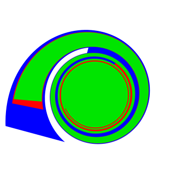
Figure 1: Strictly shrinking domains which converge to a domain not of Schoenfliess type

Address:

Florian Bauer, Daniela Kraus and Oliver Roth

Institut für Mathematik

Universität Würzburg

Am Hubland

97074 Würzburg

Germany

Elias Wegert,

Institut für Angewandte Analysis

TU Bergakademie Freiberg

Prüferstr. 9

09596 Freiberg

Germany

References

- [1] M. L. Agranovsky and T. M. Bandman, Remarks on a Conjecture of Ruscheweyh, Complex Variables (1996), 31, 249–258.
- [2] H. W. Alt and L. A. Caffarelli, Existence and regularity for a minimum problem with free boundary, J. Reine Angew. Math. (1981), 325, 105–144.
- [3] F. G. Avkhadiev and L. I. Shokleva, Generalizations of certain Beurling’s theorem with applications for inverse boundary value problem, Russ. Math. (1994), 38, No. 5, 78–81.
- [4] F. G. Avkhadiev, Conformal mappings that satisfy the boundary condition of equality of metrics, Dokl. Math. (1996), 53, No. 2, 194–196.
- [5] A. Beurling, An extension of the Riemann mapping theorem, Acta Math. (1953), 90, 117–130.
- [6] A. Beurling, On free–boundary problems for the Laplace equations, Sem. analytic functions (1958), 1, 248–263.
- [7] P. L. Duren, Theory of Spaces, Dover Publications, Mineola, New York, 2000.
- [8] P. L. Duren, H. S. Shapiro and A. L. Shields, Singular measures and domains not of Smirnov type, Duke Math. J. (1966), 33, 247–254.
- [9] J. Feng, T. H. MacGregor, Estimates on integral means of the derivatives of univalent functions, Journal d’Anal. Math. (1976), 29, 203–231.
- [10] R. Fournier and St. Ruscheweyh, Free boundary value problems for analytic functions in the closed unit disk, Proc. Amer. Math. Soc. (1999), 127 no. 11, 3287–3294.
- [11] R. Fournier and St. Ruscheweyh, A generalization of the Schwarz–Carathéodory reflection principle and spaces of pseudo–metrics, Math. Proc. Cambridge Phil. Soc. (2001), 130, 353–364.
- [12] J. B. Garnett, Bounded analytic functions, Springer, 2007.
- [13] J. B. Garnett and D. E. Marshall, Harmonic Measure, Cambrige University Press, 2005.
- [14] B. Gustafsson and H. Shahgholian, Existence and geometric properties of solutions of a free boundary problem in potential theory, J. Reine Angew. Math. (1996), 473, 137–179.
- [15] A. E. Gwilliam, On Lipschitz conditions, Proc. London Math. Soc. (1936), 40, 353–364.
- [16] A. Henrot, Subsolutions and supersolutions in a free boundary problem, Ark. Mat. (1994), 32 no. 1, 79–98.
- [17] J. M. Huntey, N. J. Moh and D. E. Tepper, Uniqueness theorems for some free boundary problems in univalent functions, Complex Variables, Theory Appl. (2003), 48 no. 7, 607–614.
- [18] D. Kinderlehrer and L. Nirenberg, Regularity in free boundary problems, Ann. Sc. Norm. Super. Pisa, Cl. Sci. (1977) IV Ser. 4, 373–391.
- [19] D. Kraus and O. Roth, Critical points of inner functions, nonlinear partial differential equations, and an extension of Liouville’s theorem, to appear in J. London Math. Soc.
- [20] R. Kühnau, Längentreue Randverzerrung bei analytischer Abbildung in hyperbolischer und sphärischer Geometrie, Mitt. Math. Sem. Giessen (1997), 229, 45–53.
- [21] Ch. Pommerenke, Boundary behaviour of conformal maps, Springer, 1992.
- [22] O. Roth, A general conformal geometric reflection principle, Trans. Amer. Math. Soc. (2007), 359 No. 6, 2501–2529.
- [23] M. Sakai, Regularity of a boundary having a Schwarz function, Acta Math. (1991), 166 no. 3/4, 263–297.
- [24] M. Sakai, Regularity of boundaries of quadrature domains in two dimensions, SIAM J. Math. Anal. (1993), 24 no. 2, 341–364.
- [25] E. Wegert, Nonlinear Boundary Value Problems for Holomorphic Functions and Singular Integral Equations, Akademie Verlag Berlin, 1992.