Variability in the Prompt Emission of Swift-BAT Gamma-Ray Bursts

Abstract

We present the results of our study of the variability time scales of a sample of 27 long Swift Gamma-Ray Bursts (GRBs) with known redshifts. The variability time scale can help our understanding of fundamental GRB parameters such as the initial bulk Lorentz factor and the characteristic size associated with the emission region. Fast Fourier Transform (FFT) techniques were used to extract a noise threshold crossing frequency, which we associate with a variability time scale. The threshold frequency appears to show a correlation with the peak isotropic luminosity of GRBs.

1 Introduction

The time variability in Gamma-ray Bursts (GRBs) is crucial to our understanding of the characteristic size associated with GRBs.

In 2000, Fenimore and Ramirez-Ruiz first proposed a correlation between variability of GRBs and peak isotropic luminosity Fenimore & Ramirez-Ruiz (2000). Since then a number of authors have provided further support for this correlation Reichart et al. (2001); Guidorzi (2005); Guidorzi et al. (2005, 2006); Li & Paczyński (2006); Rizzuto et al. (2007). However, these authors used a variety of definitions for variability with various parameters and smoothing methods. The lack of a universally accepted definition for variability is a major short coming and poses problems in comparing and evaluating the results of previous studies.

In our analysis we have used Fourier analysis techniques to probe various frequencies and their strength in GRB light curves. In this paper we associate a threshold frequency, which is the frequency where the signal crosses the noise level, as a potential variability indicator.

Due its fast slewing capability, the $Swift$ Gamma-Ray Burst mission Gehrels et al. (2004) has enabled more redshift measurements of GRBs than before. With its highly sensitive primary instrument, the Burst Alert Telescope (BAT) (Barthelmy et al., 2005), $Swift$ provides high quality GRB data on which a Fourier analysis can be performed and a variability time scale extracted. Our sample contains 27 $Swift$ BAT GRBs with good spectral measurements. We extracted the threshold frequency for all the GRBs and show this parameter is correlated with the isotropic peak luminosity.

2 Methodology

The discrete Fourier transform of a series of N counts or numbers is given by

$$x_{k}=\frac{1}{N}\sum_{j=-N/2}^{N/2-1}a_{j}\,e^{-2\pi\,ij\,k/N},\,\,\,\,\,k=0,...,N-1;\,\,\,\,\,\ a_{j}=\sum_{k=0}^{N-1}x_{k}\,e^{2\pi\,ij\,k/N},\,\,\,\,\,j=-\frac{N}{2},...,\frac{N}{2}-1$$ (1)

To calculate the power spectrum, the Fast Fourier Transform (FFT) algorithm was used (Jenkins and Watts, 1968). The power spectrum is defined as Leahy et al. (1983)

$$P_{j}\equiv\frac{2}{\sum x_{k}}\,|a_{j}|^{2},\,\,\,\,\,\,j=0,\,...,\frac{N}{2}.$$ (2)

We have used BAT event-by-event data and utilized the “IDL Extract” software package to generate power spectra for our analysis. We divided the burst into 2 segments and averaged the corresponding power spectra to get the final spectra. A typical power spectrum from a GRB is shown in Fig. 1. The low frequency power-law component, sometimes referred to as “red noise”, represents the signal from the source. The high frequency region, called “white noise”, is background. The threshold frequency, $f_{\rm th}$, is the frequency at which the red noise crosses the white noise level. In order to extract the threshold frequency, the power spectra were fitted by a broken power law

$$P=\left\{\begin{array}[]{ll}A\big{(}f/f_{\rm th}\big{)}^{-\alpha},&f<f_{\rm th},\\ A\big{(}f/f_{\rm th}\big{)}^{-\beta},&\rm otherwise.\end{array}\right.$$

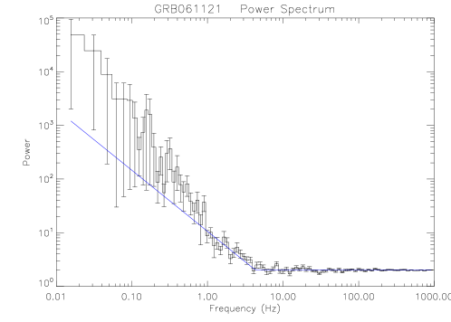
Figure 1: The power as a function of frequency. A broken power-law is fitted to the power spectrum to obtain the threshold frequency where the red noise (source signal) intersects the white noise (background).

When calculating the isotropic peak luminosity ($L_{\rm iso}$), we need to take into account the fact that in the rest frame of the GRB, photon energies are higher than those in the observer frame. The observed peak flux for the source–frame energy range $1.0\,\rm{keV}$ to $10,000\,\rm{keV}$ was calculated using observed spectral-fit parameters for the GRB sample and appropriately z-corrected energy limits in the integral. The isotropic peak luminosity is related to the calculated flux as follows:

$$L_{\rm iso}=4\pi d_{L}^{\,2}\,F_{\rm{obs}}.$$ (3)

Here $F_{\rm{obs}}$ is the observed peak flux and the luminosity distance, $d_{L}$, is given by,

$$d_{L}=\frac{(1+z)c}{H_{0}}\int_{0}^{z}\frac{dz}{\sqrt{\Omega_{M}(1+z)^{3}+\Omega_{k}(1+z)^{2}+\Omega_{L}}}.$$ (4)

For the current universe we have assumed, $\Omega_{M}=0.27$, $\Omega_{L}=0.73$, $\Omega_{k}=0.0$ and a Hubble constant ($H_{0}$) of $70\,\rm\,km\,s^{-1}\,Mpc^{-1}\,=\,2.268\times 10^{-18}\,\rm s^{-1}$. The redshift measurements were taken from online archives of the Gamma-Ray Burst Online Index (GRBOX) and verified by using the GCN circulars.

3 Results

From a sample of 100 $Swift$ BAT GRBs with spectroscopically confirmed redshifts, we selected 27 GRBs with good spectral measurements. We analyzed event-by-event data of this sample and obtained power spectra and fitted these with a broken power law and extracted the threshold frequencies. We find the average $\alpha$ for the sample is $1.12\pm 0.05$ and $\beta$ is consistent with zero for all fits. In Fig. 2 panel (a), we show the calculated isotropic peak luminosity as a function of the extracted threshold frequency (with the appropriate z correction). As seen in the figure, the threshold frequency appears to be correlated with the isotropic peak luminosity. The Pearson’s correlation coefficient is $0.69\pm 0.03$, where the uncertainty was obtained through a Monte Carlo simulation. The probability that the above correlation occurs due to random chance is $3.4\times 10^{-4}$. Our best-fit yields the following relation between $L_{\rm iso}$ and $f_{\rm th}$:

$$\log L_{\rm iso}=(52.0\pm 0.2)+(1.4\pm 0.2)\log(f_{\rm th}(z+1)).$$ (5)

Panel (b) in Fig. 2 shows a histogram of the threshold frequencies. The lowest redshift-corrected threshold frequency in the sample is approximately 0.2 Hz and the largest is about 20 Hz. Our results imply the smallest variability time scale to be approximately 50 msec.

Figure 2: Panel (a): Isotropic peak luminosity as a function of threshold frequency. The correlation coefficient of the relation is $0.69\pm 0.03$ with a chance probability of $3.4\times 10^{-4}$. Panel (b): Distribution of the time-dilation-corrected threshold frequencies.

4 Discussion

It is important to investigate how the observed brightness of GRBs affects the extracted threshold frequencies because the threshold frequency also appears to be correlated with the observed brightness (see Fig. 3 panel (a)) and this potential observational bias needs further investigation.

FFT power is roughly proportional to the brightness of the burst. Hence when a burst of a given luminosity is closer and therefore brighter, the red noise is enhanced above the constant Poisson noise level (white noise) and results in a larger threshold frequency. Given a burst of luminosity $L_{\rm iso}$ and frequency $f_{\rm th}$, the same burst with a different luminosity $L_{\rm iso}^{\prime}$ would fall on the following $L_{\rm iso}^{\prime}-f_{\rm th}^{\prime}$ line:

$$\log L_{\rm iso}^{\prime}=\log(L_{\rm iso}/f_{\rm th}^{\alpha})+\alpha\log f_{\rm th}^{\prime}.$$ (6)

The mean value of $\alpha$ for our sample is $1.12\pm 0.05$, which does not fully explain the slope of $1.4\pm 0.2$ (see Fig. 2) obtained from the $L_{\rm iso}$-$f_{\rm th}$ correlation.

We note also that the uneven distribution of redshifts (see Fig 3 panel (b)) might play a role in the correlation with flux. Roughly half of the sample lies in the redshift range 1.5 to 3.5 where the luminosity distance changes only by factor of 2.8, hence, the correlation between $L_{\rm iso}$ and $f_{\rm th}$ partially trickles down to the flux as well.

Figure 3: Panel (a): Isotropic peak luminosity as a function of observed flux. Panel (b): The histogram of redshifts in the sample.

In conclusion, we argue that the FFT threshold frequency is a parameter that provides a suggestive measure of gamma-ray bursts variability. For the sample of 27 GRBs analyzed, our results imply the smallest variability time scale is approximately 50 milliseconds. The apparent correlation between the isotropic peak luminosity and the threshold frequency needs further investigation for observational bias. If confirmed, this correlation is potentially useful as a probe of GRB microphysics. It may also prove useful as a redshift estimator.

References

- Fenimore & Ramirez-Ruiz (2000) Fenimore, E. E., & Ramirez-Ruiz, E. 2000, arXiv:astro-ph/0004176
- Reichart et al. (2001) Reichart, D. E., Lamb, D. Q., Fenimore, E. E., Ramirez-Ruiz, E., Cline, T. L., & Hurley, K. 2001, ApJ., 552, 57
- Guidorzi (2005) Guidorzi, C. 2005, MNRAS, 364, 163
- Guidorzi et al. (2005) Guidorzi, C., Frontera, F., Montanari, E., Rossi, F., Amati, L., Gomboc, A., Hurley, K., & Mundell, C. G. 2005, MNRAS, 363, 315
- Guidorzi et al. (2006) Guidorzi, C., Frontera, F., Montanari, E., Rossi, F., Amati, L., Gomboc, A., & Mundell, C. G. 2006, MNRAS, 371, 843
- Li & Paczyński (2006) Li, L.-X., & Paczyński, B. 2006, MNRAS, 366, 219
- Rizzuto et al. (2007) Rizzuto, D., et al. 2007, MNRAS, 379, 619
- Gehrels et al. (2004) Gehrels, N., et al. 2004, ApJ., 611, 1005
- Barthelmy et al. (2005) Barthelmy, S. D., et al. 2005a, Space Sci. Rev., 120, 143
- Jenkins and Watts (1968) Jenkins, G., & Watts, D., 1968, Spectral Analysis and Its Applications (San Francisco: Holden-Day).
- Leahy et al. (1983) Leahy, D. A., Darbro, W., Elsner, R. F., Weisskopf, M. C., Kahn, S., Sutherland, P. G., & Grindlay, J. E. 1983, ApJ., 266, 160