Time Asymptotics and Entanglement Generation of Clifford Quantum Cellular Automata

Abstract

We consider Clifford Quantum Cellular Automata (CQCAs) and their time evolution. CQCAs are an especially simple type of Quantum Cellular Automata, yet they show complex asymptotics and can even be a basic ingredient for universal quantum computation. In this work we study the time evolution of different classes of CQCAs. We distinguish between periodic CQCAs, fractal CQCAs and CQCAs with gliders. We then identify invariant states and study convergence properties of classes of states, like quasifree and stabilizer states. Finally we consider the generation of entanglement analytically and numerically for stabilizer and quasifree states.

I Introduction

Quantum cellular automata (QCAs), i.e., reversible quantum systems which are discrete both in time and in space Werner2004 , and exhibit strictly finite propagation, have recently come under study from different directions. On the one hand, they serve as one of the computational paradigms for quantum computation, and it has been shown that a certain one-dimensional QCA with twelve states per cell can efficiently simulate all quantum computers Shepherd2006 . On the practical side, QCAs are a direct axiomatization of the kind of quantum simulator in optical lattices, which are under construction in many labs at the moment Bloch ; Meschede . Related to this, they can be seen as a paradigm of quantum lattice systems, in which the consequences of locality, assumed in the idealized pure form of strictly finite propagation, can be explored directly. Due to the famous Lieb-Robinson bounds Lieb1972 ; Nachtergaele ; Hastings2006 ; Eisert2006 this feature is also present in continuous time models albeit in an approximate form.

In all these settings, the time asymptotics for the iteration of the QCA is of interest, and displays a curious dichotomy between a global and a local point of view. On the one hand we are assuming reversibility, so the global evolution is an automorphism taking pure states to pure states. If we split the system into two subsystems, e.g., a right half chain and a left half chain, then we expect the QCA to generate entanglement from any initial product state. There is a simple upper bound (see Section IV.1) showing that the entanglement growth is at most linear, and we find indeed that for the automata studied in this paper this is the typical behavior. However, utilizing this entanglement requires the control of larger and larger regions. So from a local perspective, i.e., when we only consider the restriction of the state to a finite region, we will not see this increase. In fact, a typical behavior of the local restrictions is the convergence to the maximally mixed state. That for large times the state seems globally pure and locally completely mixed is no contradiction: it merely reflects the fact that any local system becomes maximally entangled with its environment.

Stationary states are in some sense the final result of an asymptotic evolution. Again the local analysis makes it clear that the totally mixed state is invariant for any reversible cellular automaton. In general there may be many more invariant states, among them some, which are not only ergodic (i.e., extremal in the set of all translation invariant states), but even pure (i.e., extremal in the set of all states). For a special class we consider here, we exhibit a rich set of such states.

The very fact that QCAs can serve as a universal computational model suggests that asymptotic questions cannot be easily answered in full generality. Therefore, in this paper we look at a subclass of QCAs, the Clifford Quantum Cellular Automata (CQCAs). In this case much of the essential information can be obtained by studying a classical cellular automaton, which even turns out to be of a linear type. Consequently, we can answer some questions exhaustively. The drawback is, of course, that universal computation is not possible in this class. However, we believe that some typical features of QCA asymptotics can be studied in this theoretical laboratory .

Our paper is organized as follows. We begin with a short introduction to CQCAs and their representation as $2\times 2$-matrices in Section II.1. Then we derive a general theory of the time evolution of CQCAs in Section II.2. We show that CQCAs can be divided in three major classes by their time evolution: periodic automata (Section II.2.2), automata which act as lattice translations on special observables we call gliders (Section II.2.1), and fractal automata (Section II.2.3), whose space-time picture shows self-similarity on large scales. The class of a CQCA is determined by the trace of its matrix. A constant trace means the automaton is periodic, a trace of the form $u^{-n}+u^{n}$ indicates gliders that move $n$ steps on the lattice each time step. All other CQCAs show fractal behavior. We prove that all automata with gliders and $n=1$ are equivalent in the sense that they can be transformed into each other by conjugation with other CQCAs. This turns out not to be true for glider CQCAs with $n>1$.

Using the results for the observable asymptotics, in Section III convergence and invariance of translation-invariant states are analyzed. For periodic CQCAs the construction of mixed invariant states is straightforward (Section III.1). There are also pure stabilizer states that are invariant with respect to periodic CQCAs (Section III.3.1). Non-periodic CQCAs can not leave stabilizer states invariant. In fact, for fractal CQCAs the only known invariant state is the tracial state. For glider CQCAs invariant states exist, and are constructed as the limit of the time evolution of initial product states in Section III.2. Finally we consider $n=1$ glider automata and states which are quasifree on the canonical anticommutation relations (CAR) algebra (Section III.4). We employ the Araki-Jordan-Wigner transformation (Section III.4.1) to transfer the glider CQCA to the CAR algebra and study its action as a Bogoliubov transformation on quasifree states; we study both convergence (Section III.4.3) and invariance (Section III.4.2).

In the last Section (Section IV) the entanglement generation of CQCAs is considered. First we derive a general linear upper bound for entanglement generation of QCAs. We then prove that in the translation-invariant case the bound is more restrictive and can be saturated by CQCAs acting on initially pure stabilizer states. For CQCAs acting on stabilizer states the asymptotic entanglement generation rate is governed by the order of the trace polynomial (Section IV.2). We then examine a set of quasifree states interpolating between a product state and a state which is invariant with respect to the standard glider CQCA (Section IV.3). It is shown numerically, that the entanglement generation is linear also in this case, but with a slope that can be arbitrarily small.

II Time evolution of the observable algebra

CQCAs show a variety of different time evolutions. In this section we develop criteria to predict the time evolution by characteristics of the matrix of the corresponding symplectic cellular automaton (SCA).

II.1 A short introduction to CQCAs

Clifford Quantum Cellular Automata are a special class of Quantum Cellular Automata first described in SchlingemannCQCA . As the name indicates, they are QCAs that use the Clifford group operations. They can be defined for arbitrary lattice dimensions and prime cell dimensions. Here we will only consider the case of a one dimensional infinite lattice and cell dimension two (qubits). Thus we deal with an ordinary spin-chain. QCAs are translation-invariant operations which we define on a quasi-local observable algebra Werner2004 . Reversible QCAs are automorphisms. So in our case CQCAs are translation-invariant automorphisms of the spin-$\frac{1}{2}$ chain observable algebra $\mathfrak{A}=\otimes_{i=-\infty}^{\infty}\mathfrak{A}_{i}$, where $\mathfrak{A}_{i}\cong M_{2}$. In explicit this means that a CQCA $T$ commutes with the lattice translation $\tau$ and leaves the product structure of observables invariant:

$$T(AB)=T(A)T(B),\quad\forall A,B\in\mathfrak{A}$$

As shown in Werner2004 a QCA is fully specified by its local transition rule $T_{0}$, i.e., the picture of the one-site observable algebra. In our case the Pauli matrices form a basis of this algebra, so their pictures specify the whole CQCA. There is one important restriction on the set of possible images. They have to fulfill the commutation relations of the original Pauli matrices on the same site and also on all other sites. As a QCA in general has a propagation on the lattice, one cell observables are mapped to observables on a neighborhood $\mathcal{N}$ of the site. Thus neighboring one-site observables may overlap after one time step but still have to commute. This imposes conditions on the local rule. CQCAs are defined as follows:

Definition II.1.

A Clifford Quantum Cellular Automaton $T$ is an automorphism of the quasi-local observable algebra of the infinite spin chain that maps tensor products of Pauli matrices to multiples of tensor products of Pauli matrices and commutes with the lattice translation $\tau$.

We now want to find a classical description of the CQCA. It is well known that Clifford operations can be simulated efficiently by a classical computer. Therefore it is not surprising that an efficient classical description of CQCAs exists. This description was introduced in SchlingemannCQCA . We will only give a short overview of the topic, for proofs and details we refer to the literature.

We use the (finite) tensor products of Pauli matrices as a basis of the observable algebra. Every CQCA $T$ maps those tensor products to multiples of tensor products of Pauli matrices. The factor can only be a complex phase, that can be fixed uniquely by the phase for single cell observables (single Pauli matrices). We can thus describe the action of the CQCA $T$ on Pauli matrices by a classical cellular automaton t acting on their labels “$1,2,3$”. We could keep track of the phase separately, but for our analysis this is unnecessary.

Mathematically we describe this correspondence as follows: The Pauli matrices correspond to a Weyl system over a discrete phase space where all operations are carried out modulus two. For one site we have

$$\sigma_{1}=X={\bf w}(1,0),\quad\sigma_{2}=Y=i{\bf w}(1,1),\quad\sigma_{3}=Z={\bf w}(0,1),\quad\sigma_{0}=\mathds{1}={\bf w}(0,0).$$

Tensor products of these operators are constructed via

$${\bf w}(\xi)=\bigotimes_{x\in\mathbb{Z}}{\bf w}(\xi(x))$$

where $\xi=(\xi_{+},\xi_{-})$ is a tuple of two binary strings which differ from $0$ on only finitely many places and $\xi(x)$ is its value at position $x$, e.g. $\tbinom{1}{0}$. Thus the tensor product is well defined. Before we continue with the mathematical definition, we want to illustrate the classical description by a simple example:

Example II.2.

We define our CQCA on the observable algebra $\mathfrak{A}$ of a spin chain by the rule

$$\begin{array}[]{rcc}&T_{i}:&\mathfrak{A}_{i}\to\mathfrak{A}_{\mathcal{N}+i},\\ T\sigma_{1}^{i}&=&\sigma_{3}^{i},\\ T\sigma_{3}^{i}&=&\sigma_{3}^{i-1}\otimes\sigma_{1}^{i}\otimes\sigma_{3}^{i+1}.\end{array}$$

The image of $\sigma_{2}$ follows from the product of the images of $\sigma_{1}$ and $\sigma_{3}$:

$$T\sigma_{2}^{i}=-\sigma_{3}^{i-1}\otimes\sigma_{2}^{i}\otimes\sigma_{3}^{i+1}.$$

$T$ has to be an automorphism to be a CQCA. To verify this we check if the commutation relations are preserved:

$$\phantom{b}[T\sigma_{1}^{i},T\sigma_{1}^{j}] = [\sigma_{3}^{i},\sigma_{3}^{j}]=0,$$

$$\phantom{b}[T\sigma_{3}^{i},T\sigma_{3}^{j}] = [\sigma_{3}^{i-1}\otimes\sigma_{1}^{i}\otimes\sigma_{3}^{i+1},\sigma_{3}^{j-1}\otimes\sigma_{1}^{j}\otimes\sigma_{3}^{j+1}]=0,$$

and

$$[T\sigma_{3}^{i},T\sigma_{1}^{j}]=[\sigma_{3}^{i-1}\otimes\sigma_{1}^{i}\otimes\sigma_{3}^{i+1},\sigma_{3}^{j}]=0 i\neq j,$$

$$\{T\sigma_{3}^{i},T\sigma_{1}^{j}\}=\{\sigma_{3}^{i-1}\otimes\sigma_{1}^{i}\otimes\sigma_{3}^{i+1},\sigma_{3}^{j}\}=0 i=j\;.$$

This automaton will be used extensively in the following parts of the paper, so we give it the name $G_{s}$. If we think of the CQCA $G_{s}$ as a classical automaton acting on the labels of the Pauli matrices we can illustrate the evolution (for one time step) of the observable $\sigma_{3}^{-1}\otimes\sigma_{2}^{0}\otimes\sigma_{1}^{1}$ as follows (the underlined labels are situated at the origin):

$$\textbf{\emph{g}}_{s}(3\,\underline{2}\,1)=\textbf{\emph{g}}_{s}(3\,\underline{0}\,0)\cdot\textbf{\emph{g}}_{s}(0\,\underline{2}\,0)\cdot\textbf{\emph{g}}_{s}(0\,\underline{0}\,1)=\begin{array}[]{ccccc}&3&1&\underline{3}&\\ \odot&&3&\underline{-2}&3\\ \odot&&&&3\\ \hline\cr=&3&-i2&\underline{i1}&0\end{array}=(3\,2\,\underline{1}).$$

We observe, that the observable only moves on the lattice under the action of the CQCA $T$. We call observables with this property gliders. Their existence can be observed easily, when we consider the space-time images of one-cell observables. $\sigma_{1}$ and $\sigma_{3}$ generate “checkerboards” of $\sigma_{1}$ and $\sigma_{3}$ matrices. As $\sigma_{1}$ is mapped to $\sigma_{3}$ in the first step, the $\sigma_{1}$-checkerboard is the same as the $\sigma_{3}$-checkerboard shifted one step in time. If we additionally shift in the space direction by one cell, the checkerboards are exactly the same up to two diagonals and thus cancel out as shown in Figure 1. We thus produced a very simple observable on which the automaton acts as a translation, a basic glider.

Figure 1: Glider of the example CQCA (4). The blue boxes represent $\sigma_{1}$, the yellow ones $\sigma_{3}$.

Another interesting property of this automaton is the fact that it maps the “all spins up” product state to a one-dimensional cluster-state, which is a one-dimensional version of the two-dimensional resource-state for the “One Way Quantum Computing” scheme by Raussendorf and Briegel Raussendorf2001 . It is also the basic ingredient of a scheme of “quantum computation via translation-invariant operations on a chain of qubits” by Raussendorf Raussendorf2005a . In a similar way, the update rule $G_{s}$ (but with $\sigma_{1}$ and $\sigma_{3}$ exchanged) has appeared as time-evolution of spin chains implemented by a Hamiltonian that is subjected to periodic quenches fitzsimons2006 ; eisler , and it has even been realized experimentally in an NMR-System fitzsimons2007 .

In the phase space picture we can describe the automaton by a $2\times 2$-matrix with polynomial entries. In phase space our CQCA-rule reads

$$\textbf{\emph{g}}_{s}\binom{1}{0} = \left(\begin{array}[]{ccc}0&0&0\\ 0&1&0\end{array}\right),$$

$$\textbf{\emph{g}}_{s}\binom{0}{1} = \left(\begin{array}[]{ccc}0&1&0\\ 1&0&1\end{array}\right),$$

$$\textbf{\emph{g}}_{s}\binom{1}{1} = \left(\begin{array}[]{ccc}0&1&0\\ 1&1&1\end{array}\right).$$

Now we transform the binary strings to Laurent polynomials by indicating the position by a multiplication with a variable $u$ and add all terms from the different positions to a Laurent polynomial:

$$\textbf{\emph{g}}_{s}\binom{1}{0} = \binom{0}{1},$$

$$\textbf{\emph{g}}_{s}\binom{0}{1} = \binom{1}{u^{-1}+u},$$

$$\textbf{\emph{g}}_{s}\binom{1}{1} = \binom{1}{u^{-1}+1+u}.$$

We arrange the images of $\tbinom{1}{0}$ and $\tbinom{0}{1}$ in a $2\times 2$-matrix

$$\textbf{\emph{g}}_{s}=\left(\begin{array}[]{cc}0&1\\ 1&u^{-1}+u\end{array}\right).$$ (4)

The image under $G_{s}$ of an arbitrary tensor product of Pauli matrices is now determined by the multiplication of the corresponding vector of polynomials by the matrix representation $\textbf{\emph{g}}_{s}$ of $G_{s}$. We will later argue that this works for all CQCA. $\lozenge$

Now we come back to the mathematical definition of CQCAs: The Weyl operators fulfill the relation

$${\bf w}(\xi+\eta)=(-1)^{\eta_{+}\xi_{-}}{\bf w}(\xi){\bf w}(\eta)$$

and therefore the commutation relation

$${\bf w}(\xi){\bf w}(\eta)=(-1)^{\xi_{+}\eta_{-}-\xi_{-}\eta_{+}}{\bf w}(\eta){\bf w}(\xi).$$

In both cases terms of the type $\xi_{+}\eta_{-}$ are scalar products where the addition is carried out modulo $2$. The arguments of the Weyl operators are elements of a vector space over the finite field $\mathbb{Z}_{2}$ which we call phase space and thus commute. Of course the corresponding Weyl operators do not necessarily commute, but they always commute or anticommute. Their commutation relations are encoded in the symplectic form $\sigma(\xi,\eta)=\beta(\xi,\eta)-\beta(\eta,\xi)=\xi_{+}\eta_{-}-\xi_{-}\eta_{+}\in\mathbb{Z}_{2}$. As an automorphism the CQCA leaves the commutation relations invariant. A representation of the CQCA on phase space therefore has to leave the symplectic form invariant. Such a translation-invariant symplectic map is called symplectic cellular automaton (SCA). We can find a SCA and an appropriate phase function $\lambda({\xi})$ for every CQCA.

Proposition II.3 (SchlingemannCQCA ).

Let $T$ be a CQCA. Then we can write

$$T[{\bf w}(\xi)]=\lambda({\xi}){\bf w}({\textbf{\emph{t}}}\xi)$$ (5)

with a symplectic cellular automaton t and a translation invariant phase function $\lambda({\xi})$ which fulfills

$$\lambda({\xi+\eta})=\lambda({\xi})\lambda({\eta})(-1)^{\beta(\xi,\eta)-\beta({\textbf{\emph{t}}}\xi,{\textbf{\emph{t}}}\eta)}$$

as well as $|\lambda({\xi})|=1\;\forall\xi$. Furthermore, $\lambda(\xi)$ is uniquely determined for all $\xi$ by the choice of $\lambda$ on one site.

In the following analysis of CQCAs we neglect the global phase and consider the symplectic cellular automata only. As we can always find appropriate phase functions all results for SCAs translate to the world of CQCAs directly. We have already seen in Example II.2, that there exists a very convenient representation of CQCAs as $2\times 2$-matrices with polynomial entries.

Definition II.4.

${\mathcal{P}}$ is the ring of Laurent polynomials over $\mathbb{Z}_{2}$. ${\mathcal{R}}$ is the subring of ${\mathcal{P}}$, which consists of all polynomials, which are reflection invariant with center $u=0$.

Theorem II.5.

Every CQCA $T$ is represented up to a phase by a unique $2\times 2$-matrix t with entries from ${\mathcal{P}}$. Such a matrix represents a CQCA if and only if

• $\det({\textbf{\emph{t}}})=u^{2a},\,a\in\mathbb{Z}$;

• all entries are symmetric polynomials centered around the same (but arbitrary) lattice point $a$;

• the entries of both column vectors, which are the pictures of $(1,0)$ and $(0,1)$, are coprime.

Proof.

We will only give a sketch of the proof. For details see SchlingemannCQCA . The connection between CQCAs and SCAs was already established in Proposition II.3. What remains to show is that SCAs are linear transformations over ${\mathcal{P}}^{2}$. The application of a SCA to a vector in phase space can be described as the multiplication of this vector with a matrix representing the SCA from the left. The product is the convolution of binary strings. By the algebraic Fourier transform $\hat{f}(u)=\sum_{x\in\mathbb{Z}}f(x)u^{x}$, which maps the vectors of binary strings onto vectors with entries from the ring ${\mathcal{P}}$ of Laurent polynomials over the finite field $\mathbb{Z}_{2}$, the convolution of strings translates into the multiplication of polynomials. Thus in this picture the application of the SCA to a phase space vector is just a common matrix multiplication, where all operations are carried out modulo $2$. If we translate the symplectic form and the condition that it has to be left invariant to the polynomial picture we retrieve the above conditions on the matrix t. ∎

We can further simplify these statements by only considering automata centered around $0$. The lattice translation $\tau$ is a SCA which by definition commutes with all other SCAs. Its determinant is given by $\det(\tau)=u^{2}$. Therefore every SCA can be written as the product of a lattice translation and an automaton centered around $0$ which has determinant one. We call these automata centered symplectic cellular automata (CSCAs) and in the following sections we point our focus to those.

CSCAs and CQCAs each form a group. This group is generated by a countably infinite set of basis automata. The CSCA form the group $\Gamma={\rm SL}(2,{\mathcal{R}})$, which is the group of all $2\times 2$-matrices with determinant $1$ over the ring of centered Laurent polynomials with binary coefficients. The group $\Gamma_{0}$ is the group of local automata. Their generators are

$$H={\left(\begin{array}[]{cc}1&0\\ 1&1\end{array}\right)},\quad P={\left(\begin{array}[]{cc}0&1\\ 1&0\end{array}\right)}.$$

Additionally we have the shear transformations

$$G_{n}:={\left(\begin{array}[]{cc}1&0\\ {u^{n}+u^{-n}}&1\end{array}\right)},\,n\in\mathbb{N}.$$

which complete the set of generators of $\Gamma$. For proofs see SchlingemannCQCA .

II.2 Classification of Clifford quantum cellular automata

The time evolution of a CQCA is determined up to a phase by the powers of the matrix of the corresponding CSCA. We will only consider the evolution of single cell observables, as any other observable can be represented by products and sums of these. This product structure is invariant under the action of the automaton, because it is an automorphism of the observable algebra. This means that when we discuss the time evolution of a CQCA $T$, we will consider the action of powers ${\textbf{\emph{t}}}^{n}$ of the matrix of the CSCA on phase space vectors which only contain constants. For example the image of $\sigma_{1}={\bf w}(1,0)$ after $n$ time steps of $T$ is given by the first column vector of ${\textbf{\emph{t}}}^{n}$ (and a global phase). The matrix t does not always have an eigenvalue, because it is a matrix over a ring without multiplicative inverses for all elements. But for some of the automata eigenvalues do exist. These automata are called glider-automata, because on a special set of observables, the gliders, they act as lattice translations.

We will prove that if the trace is a polynomial consisting of only two summands, i.e., it is of the form $\mathrm{tr}\,{\textbf{\emph{t}}}=u^{-n}+u^{n}$, two eigenvectors exist and the automaton has gliders. If this does not hold, we can distinguish two cases. The trace can be either a constant, or an arbitrary symmetric polynomial. In the first case the automaton is periodic, in the second case it generates a time evolution which has fractal properties. As the case of periodic automata is not very interesting and the case of fractal automata will be covered in another paper Nesme , we focus on automata with gliders. We prove that all automata with gliders which move one step on the lattice at every timestep are equivalent. We also give an example to show that this is not the case for gliders that move more than one step.

II.2.1 Automata with gliders

We will first define our notion of a glider. Here we consider the case of qubits only, but with minor alterations all results of this section also hold for qudits with prime dimension. This extension and also all proofs which are omitted here can be found in Guetschow2008a ; Uphoff2008 .

Definition II.6.

A glider is an observable, on which the CQCA acts as a lattice translation. In the Laurent polynomial picture a translation is a multiplication by $u^{k},\,k\in\mathbb{Z}$.

We have already seen this behavior in Example II.2. Now we determine the conditions a CQCA has to fulfill to have gliders. In general we can not diagonalize the matrices of the corresponding CSCA, because all our calculations are over a finite field and the entries are only polynomials in $u$ which are centered palindromes. The polynomials are usually not invertible, so the equations which occur in the diagonalization cannot be solved mechanically. Furthermore, the diagonal matrix would not correspond to a CSCA as $u^{n}$ and $u^{-n}$ are not centered palindromes. Hence we take a different approach. First, let us introduce some terms: We call a glider $\xi=(\xi_{+},\xi_{-})$ a minimal glider iff its two entries in phase space $\xi_{+}$, $\xi_{-}$ have no common non-invertible divisor. The wedge-product of two phase space vectors shall be defined as $\xi\wedge\eta=\xi_{+}\eta_{-}-\eta_{+}\xi_{-}$. As we deal with qubits here, addition and multiplication of polynomials are carried out modulo two and $\xi\wedge\eta=\xi_{+}\eta_{-}+\eta_{+}\xi_{-}$. We define the involution of a polynomial $p$ as the substitution of $u$ by $u^{-1}$ and denote it by $\bar{p}$. Finally we will also need the following proposition:

Proposition II.7 (Guetschow2008a ; Uphoff2008 ).

In the ring ${\mathcal{P}}$ of Laurent polynomials over the finite field $\mathbb{Z}_{2}$, the only invertible elements are monomials.

Now we have all we need to state following theorems:

Proposition II.8.

Given a CSCA t and a non-zero phase space vector $\xi$ with ${\textbf{\emph{t}}}\xi=u^{n}\xi$, $n\in\mathbb{N}$ the following is true:

1. $\bar{\xi}$ fulfills ${\textbf{\emph{t}}}\bar{\xi}=u^{-n}\bar{\xi}$, thus it is a glider with the same speed but different direction as $\xi$.

2. t is uniquely given by

   $${\textbf{\emph{t}}}_{11} = \frac{u^{n}\xi_{+}\bar{\xi}_{-}+u^{-n}\bar{\xi}_{+}\xi_{-}}{\xi\wedge\bar{\xi}},$$ (6)

   $${\textbf{\emph{t}}}_{12} = \frac{\left(u^{n}+u^{-n}\right)\,\xi_{+}\bar{\xi}_{+}}{\xi\wedge\bar{\xi}},$$ (7)

   $${\textbf{\emph{t}}}_{21} = \frac{\left(u^{n}+u^{-n}\right)\,\xi_{-}\bar{\xi}_{-}}{\xi\wedge\bar{\xi}},$$ (8)

   $${\textbf{\emph{t}}}_{22} = \frac{u^{-n}\xi_{+}\bar{\xi}_{-}+u^{n}\bar{\xi}_{+}\xi_{-}}{\xi\wedge\bar{\xi}}.$$ (9)

3. $tr({\textbf{\emph{t}}})=u^{-n}+u^{n}$

4. All gliders are multiples of

   $$\xi=\binom{\xi_{+}}{\xi_{-}}=\binom{\frac{{\textbf{\emph{t}}}_{12}}{\mathrm{gcd}\left(u^{n}+{\textbf{\emph{t}}}_{11},{\textbf{\emph{t}}}_{12}\right)}}{\frac{u^{n}+{\textbf{\emph{t}}}_{11}}{\mathrm{gcd}\left(u^{n}+{\textbf{\emph{t}}}_{11},{\textbf{\emph{t}}}_{12}\right)}},$$ (10)

   or

   $$\bar{\xi}=\binom{\bar{\xi}_{+}}{\bar{\xi}_{-}}=\binom{\frac{{\textbf{\emph{t}}}_{12}}{\mathrm{gcd}\left(u^{-n}+{\textbf{\emph{t}}}_{11},{\textbf{\emph{t}}}_{12}\right)}}{\frac{u^{-n}+{\textbf{\emph{t}}}_{11}}{\mathrm{gcd}\left(u^{-n}+{\textbf{\emph{t}}}_{11},{\textbf{\emph{t}}}_{12}\right)}}.$$ (11)

Proof.

1. We use ${\textbf{\emph{t}}}\xi=u^{n}\xi$ and take the involution on both sides. t consists of palindromes, thus $\bar{\textbf{\emph{t}}}={\textbf{\emph{t}}}$ and we get ${\textbf{\emph{t}}}\bar{\xi}=u^{-n}\bar{\xi}$.

2. We write ${\textbf{\emph{t}}}\xi=u^{n}\xi$ and ${\textbf{\emph{t}}}\bar{\xi}=u^{-n}\bar{\xi}$ component wise yielding the four equations

   $$\begin{array}[]{crcl}(\mathrm{I})&{\textbf{\emph{t}}}_{11}\xi_{+}+{\textbf{\emph{t}}}_{12}\xi_{-}&=&u^{n}\xi_{+},\\ (\mathrm{II})&{\textbf{\emph{t}}}_{21}\xi_{+}+{\textbf{\emph{t}}}_{22}\xi_{-}&=&u^{n}\xi_{-},\\ (\bar{\mathrm{I}})&{\textbf{\emph{t}}}_{11}\bar{\xi}_{+}+{\textbf{\emph{t}}}_{12}\bar{\xi}_{-}&=&u^{-n}\bar{\xi}_{+},\\ (\bar{\mathrm{II}})&{\textbf{\emph{t}}}_{21}\bar{\xi}_{+}+{\textbf{\emph{t}}}_{22}\bar{\xi}_{-}&=&u^{-n}\bar{\xi}_{-}.\end{array}$$

   Combining them in the right way we get

   $${\textbf{\emph{t}}}_{11}\left(\xi\wedge\bar{\xi}\right) = u^{n}\xi_{+}\bar{\xi}_{-}+u^{-n}\bar{\xi}_{+}\xi_{-},$$ (12)

   $${\textbf{\emph{t}}}_{12}\left(\xi\wedge\bar{\xi}\right) = \left(u^{n}+u^{-n}\right)\xi_{+}\bar{\xi}_{+},$$ (13)

   $${\textbf{\emph{t}}}_{21}\left(\xi\wedge\bar{\xi}\right) = \left(u^{n}+u^{-n}\right)\xi_{-}\bar{\xi}_{-},$$ (14)

   $${\textbf{\emph{t}}}_{22}\left(\xi\wedge\bar{\xi}\right) = u^{-n}\xi_{+}\bar{\xi}_{-}+u^{n}\bar{\xi}_{+}\xi_{-}.$$ (15)

   By assumption t is a CSCA, so the division by $\xi\wedge\bar{\xi}$ gives a polynomial result and we have Equations (6) to (9). In Proposition II.10 we will show which conditions $\xi$ has to fulfill for the division to be valid and therefore $\xi$ to be a glider.

3. $$\mathrm{tr}\,{\textbf{\emph{t}}}={\textbf{\emph{t}}}_{11}+{\textbf{\emph{t}}}_{22}=\frac{\left(\xi\wedge\bar{\xi}\right)u^{-n}+\left(\xi\wedge\bar{\xi}\right)u^{n}}{\left(\xi\wedge\bar{\xi}\right)}=u^{-n}+u^{n}$$

4. We now use $(\mathrm{I})$ and $(\mathrm{II})$ together with $\det{\textbf{\emph{t}}}=1$ and $\mathrm{tr}\,{\textbf{\emph{t}}}=u^{-n}+u^{n}$ to derive the form of $\xi$. We get the equation

   $$\xi_{+}\left(u^{n}-{\textbf{\emph{t}}}_{11}\right)=\xi_{-}{\textbf{\emph{t}}}_{12}.$$

   This equation for $\xi_{+}$ and $\xi_{-}$, has still one free parameter. One particular solution for the equation is $\xi_{+}^{(part)}={\textbf{\emph{t}}}_{12}$, $\xi_{-}^{(part)}=u^{n}-{\textbf{\emph{t}}}_{11}$. To obtain the minimal glider we have to divide these components of the particular solution by their greatest common divisor, and thus obtain (10). For (11) we do the same with $(\bar{\mathrm{I}})$ and $(\bar{\mathrm{II}})$. An arbitrary glider can be written as the glider defined by either (10) or (11) times a Laurent polynomial in $u$.

∎

Remark II.9.

We could extend our definition of gliders to observables with polynomial eigenvalues $\lambda$. These observables would be mapped to products of translates of themselves. We can show that this extension would not yield any new gliders: A CSCA t has to fulfill $\det{\textbf{\emph{t}}}=1$. With $(I)$ to $(\bar{II})$ we get

$$\det{\textbf{\emph{t}}}\cdot\left(\xi\wedge\bar{\xi}\right)^{2} = \left({\textbf{\emph{t}}}_{11}{\textbf{\emph{t}}}_{22}+{\textbf{\emph{t}}}_{12}{\textbf{\emph{t}}}_{21}\right)\cdot\left(\xi\wedge\bar{\xi}\right)^{2}$$

$$= \left(\lambda\xi_{+}\bar{\xi}_{-}+\bar{\lambda}\bar{\xi}_{+}\xi_{-}\right)\cdot\left(\bar{\lambda}\xi_{+}\bar{\xi}_{-}+\lambda\bar{\xi}_{+}\xi_{-}\right)$$

$$-\left(\left(\bar{\lambda}+\lambda\right)\xi_{+}\bar{\xi}_{+}\right)\cdot\left(\left(\lambda+\bar{\lambda}\right)\xi_{-}\bar{\xi}_{-}\right)$$

$$= \lambda\bar{\lambda}\left(\xi_{+}^{2}\bar{\xi}_{-}^{2}+2\xi_{+}\xi_{-}\bar{\xi}_{+}\bar{\xi}_{-}+\bar{\xi}_{+}^{2}\xi_{-}^{2}\right)$$

$$= \lambda\bar{\lambda}\left(\xi\wedge\bar{\xi}\right)^{2}$$

$$\Leftrightarrow\quad\det{\textbf{\emph{t}}} = \lambda\bar{\lambda}\stackrel{{\scriptstyle!}}{{=}}1$$

$$\Leftrightarrow\qquad\>\>\lambda = u^{n}.$$

The only possible solutions are $\lambda=u^{\pm n}$, $n\in\mathbb{N}$, because by Proposition II.7 in ${\mathcal{P}}$ only monomials have inverse elements. We know that $\bar{\xi}$ is always a glider to $-n$ so we only look at positive $n$. $u^{0}$ is excluded, because there is no propagation then.

Proposition II.10.

A minimal $\xi\in{\mathcal{P}}^{2}$ is a glider for a CSCA t with eigenvalue $u^{n}$, $n\in\mathbb{Z}\backslash 0$ if and only if is a divisor of $u^{-n}+u^{n}$.

Proof.

First let us assume, that $\xi$ is minimal, and $\xi\wedge\bar{\xi}$ is divisor of $u^{-n}+u^{n}$. For $\xi$ to be a glider with eigenvalue $u^{n}$, ${\textbf{\emph{t}}}\xi=\lambda\xi$ has to hold. Therefore the division in Equations (12) to (15) has to be valid. For the Equations (13) and (14) this is obviously true. For the other two equations we use a simple trick:

$${\textbf{\emph{t}}}_{11}\left(\xi\wedge\bar{\xi}\right) = u^{n}\xi_{+}\bar{\xi}_{-}+u^{-n}\bar{\xi}_{+}\xi_{-}$$

$$= u^{n}\xi_{+}\bar{\xi}_{-}+u^{-n}\bar{\xi}_{+}\xi_{-}+\underbrace{(u^{-n}\xi_{+}\bar{\xi}_{-}+u^{-n}\xi_{+}\bar{\xi}_{-})}_{=0}$$

$$= (u^{-n}+u^{n})\xi_{+}\bar{\xi}_{-}+u^{-n}\left(\xi\wedge\bar{\xi}\right)$$

Now it is apparent, that $\xi\wedge\bar{\xi}$ also divides the right hand side of (12) if it is a divisor of $u^{-n}+u^{n}$. For (15) an analogous argument holds.

Now let us show the converse. The Laurent polynomials form an Euclidean ring, which implies that the extended Euclidean algorithm is applicable simonreed . Since $\xi$ is minimal, the greatest common divisor of $\xi_{+}$ and $\xi_{-}$ is 1, according to the extended Euclidean algorithm we can chose $\eta_{+}$ and $\eta_{-}$ such that

$$\xi_{+}\eta_{-}+\xi_{-}\eta+=\gcd(\xi_{+},\xi_{-})=1.$$

Then we have:

$$\left(u^{-n}+u^{n}\right) = \left(u^{-n}+u^{n}\right)\cdot\underbrace{\left(\xi_{+}\eta_{-}+\xi_{-}\eta_{+}\right)}_{\mathrm{=1,\,as\,\xi\,min.}}\cdot\underbrace{\left(\bar{\xi}_{+}\bar{\eta}_{-}+\bar{\xi}_{-}\bar{\eta}_{+}\right)}_{\mathrm{=1,\,as\,\bar{\xi}\,min.}}$$

$$= \left(u^{-n}+u^{n}\right)\cdot\left(\xi_{+}\bar{\xi}_{+}\eta_{-}\bar{\eta}_{-}+\xi_{-}\bar{\xi}_{+}\eta_{+}\bar{\eta}_{-}+\xi_{+}\bar{\xi}_{-}\eta_{-}\bar{\eta}_{+}+\xi_{-}\bar{\xi}_{-}\eta_{+}\bar{\eta}_{+}\right)$$

$$= \left(u^{-n}+u^{n}\right)\xi_{+}\bar{\xi}_{+}\eta_{-}\bar{\eta}_{-}+\left(u^{-n}+u^{n}\right)\cdot\xi_{-}\bar{\xi}_{-}\eta_{+}\bar{\eta}_{+}$$

$$+u^{-n}\xi_{-}\bar{\xi}_{+}\eta_{+}\bar{\eta}_{-}+u^{n}\xi_{-}\bar{\xi}_{+}\eta_{+}\bar{\eta}_{-}\underbrace{+u^{-n}\xi_{+}\bar{\xi}_{-}\eta_{+}\bar{\eta}_{-}+u^{-n}\xi_{+}\bar{\xi}_{-}\eta_{+}\bar{\eta}_{-}}_{=0}$$

$$+u^{-n}\xi_{+}\bar{\xi}_{-}\eta_{-}\bar{\eta}_{+}+u^{n}\xi_{+}\bar{\xi}_{-}\eta_{-}\bar{\eta}_{+}\underbrace{+u^{-n}\bar{\xi}_{+}\xi_{-}\eta_{-}\bar{\eta}_{+}+u^{-n}\bar{\xi}_{+}\xi_{-}\eta_{-}\bar{\eta}_{+}}_{=0}$$

$$= \underbrace{\left(u^{-n}+u^{n}\right)\xi_{+}\bar{\xi}_{+}}_{={\textbf{\emph{t}}}_{12}\left(\xi\wedge\bar{\xi}\right)}\eta_{-}\bar{\eta}_{-}+\underbrace{\left(u^{-n}+u^{n}\right)\xi_{-}\bar{\xi}_{-}}_{={\textbf{\emph{t}}}_{21}\left(\xi\wedge\bar{\xi}\right)}\eta_{+}\bar{\eta}_{+}$$

$$+\underbrace{\left(u^{-n}\xi_{+}\bar{\xi}_{-}+u^{n}\xi_{-}\bar{\xi}_{+}\right)}_{={\textbf{\emph{t}}}_{22}\left(\xi\wedge\bar{\xi}\right)}\eta_{+}\bar{\eta}_{-}+\underbrace{\left(u^{n}\xi_{+}\bar{\xi}_{-}+u^{-n}\xi_{-}\bar{\xi}_{+}\right)}_{={\textbf{\emph{t}}}_{11}\left(\xi\wedge\bar{\xi}\right)}\eta_{-}\bar{\eta}_{+}$$

$$+u^{-n}\eta_{+}\bar{\eta}_{-}\left(\xi\wedge\bar{\xi}\right)+u^{-n}\eta_{-}\bar{\eta}_{+}\left(\xi\wedge\bar{\xi}\right)$$

which implies that $\xi\wedge\bar{\xi}$ divides $(u^{-n}+u^{n})$. ∎

We have shown in Proposition II.8 that $\mathrm{tr}\,{\textbf{\emph{t}}}=u^{-n}+u^{n}$ is a necessary condition for t to have gliders. The following proposition shows that this condition is also sufficient.

Proposition II.11.

A CSCA possesses gliders with eigenvalues $\lambda_{+}=u^{n}$ and $\lambda_{-}=\bar{\lambda}_{+}=u^{-n}$ if and only if $\mathrm{tr}\,{\textbf{\emph{t}}}=u^{-n}+u^{n}$.

Proof.

The “only if” part was already shown in Proposition II.8.

We now assume that $\mathrm{tr}\,{\textbf{\emph{t}}}=u^{-n}+u^{n}$ and use this to evaluate the characteristic polynomial of t. Using $\det{\textbf{\emph{t}}}=1$ we get

$$\lambda^{2}+\lambda\cdot(u^{-n}+u^{n})+1=0,$$

which is solved by $\lambda_{\pm}=u^{\pm n},\,n\in\mathbb{N}$. Thus the CSCA possesses gliders. ∎

Now that we know the conditions for the existence of gliders, we want to know how and when they can be connected. Consider an arbitrary CSCA t with gliders and a second CSCA b. If we transform t by conjugating with b we get $\widetilde{\textbf{\emph{t}}}={\textbf{\emph{b}}}^{-1}{\textbf{\emph{t}}}{\textbf{\emph{b}}}$ which has by

$$\mathrm{tr}\,\widetilde{\textbf{\emph{t}}}=\mathrm{tr}\,({\textbf{\emph{b}}}^{-1}{\textbf{\emph{t}}}{\textbf{\emph{b}}})=\mathrm{tr}\,(\mathds{1}{\textbf{\emph{t}}})=\mathrm{tr}\,{\textbf{\emph{t}}}$$

the same trace as t and thus is a glider automorphism, too. What is maybe more surprising is that the converse is also true for gliders of propagation speed one: any CSCA with one-step gliders is equivalent to the standard-glider CSCA $\textbf{\emph{g}}_{s}$ (4) by the equivalence relation $\widetilde{\textbf{\emph{t}}}={\textbf{\emph{b}}}^{-1}\textbf{\emph{g}}_{s}{\textbf{\emph{b}}}$.

Theorem II.12.

Let $\xi=\left(\xi_{+},\,\xi_{-}\right)\,\in\,{\mathcal{P}}^{2}$ be minimal. Then the following three statements are equivalent:

1. There is a CSCA t with ${\textbf{\emph{t}}}\xi=u\xi$.

2. There is a CSCA b with ${\textbf{\emph{b}}}\xi=\tbinom{1}{u}$.

3. $\xi\wedge\bar{\xi}=\left(u^{-1}+u\right)$.

Proof.

$3\Leftrightarrow 1$ has already been shown in Proposition II.10.

$1\Rightarrow 2$: We assume that 1 (and therefore also 3) is true and analyze the conditions this imposes on b: We know that ${\textbf{\emph{b}}}=\bar{\textbf{\emph{b}}}$. We start with the assumption ${\textbf{\emph{b}}}\xi=\tbinom{1}{u}$ and obtain

$${\textbf{\emph{b}}}_{11}\left(\xi\wedge\bar{\xi}\right) = \xi_{-}+\bar{\xi}_{-},$$ (16)

$${\textbf{\emph{b}}}_{12}\left(\xi\wedge\bar{\xi}\right) = \xi_{+}+\bar{\xi}_{+},$$ (17)

$${\textbf{\emph{b}}}_{21}\left(\xi\wedge\bar{\xi}\right) = \left(u^{-1}\xi_{-}+u\bar{\xi}_{-}\right),$$ (18)

$${\textbf{\emph{b}}}_{22}\left(\xi\wedge\bar{\xi}\right) = \left(u^{-1}\xi_{+}+u\bar{\xi}_{+}\right).$$ (19)

First we need to show that the matrix b actually exists, i.e., that all the right sides of the equations (16) to (19) can be divided by $\xi\wedge\bar{\xi}$. This follows from the same argument as in Proposition II.10 if $\mathrm{tr}\,{\textbf{\emph{t}}}=u^{-1}+u$, which is given by $1\Leftrightarrow 3$. For the matrix to be a CSCA the determinant has to be one. This is also true and can be shown by direct computation:

$$\det{\textbf{\emph{b}}} = \frac{1}{\left(\xi\wedge\bar{\xi}\right)^{2}}\cdot\left(\left(\xi_{-}+\bar{\xi}_{-}\right)\cdot\left(u^{-1}\xi_{+}+u\bar{\xi}_{+}\right)+\left(u^{-1}\xi_{-}+u\bar{\xi}_{-}\right)\cdot\left(\xi_{+}+\bar{\xi}_{+}\right)\right)$$

$$= \frac{1}{\left(\xi\wedge\bar{\xi}\right)^{2}}\cdot\left(u^{-1}+u\right)\cdot\left(\xi\wedge\bar{\xi}\right)$$

$$= \frac{\left(u^{-1}+u\right)}{\xi\wedge\bar{\xi}}=1$$

This step only works for $\xi\wedge\bar{\xi}=(u^{-1}+u)$ which corresponds to one step gliders. Later on we will consider gliders with higher propagation speed and give counterexamples to similar notions of equivalence for their automata.

$2\Rightarrow 3$:

$$\xi\wedge\bar{\xi}=\underbrace{\det{\textbf{\emph{b}}}}_{=1}\cdot(\xi\wedge\bar{\xi})={\textbf{\emph{b}}}\xi\wedge{\textbf{\emph{b}}}\bar{\xi}=\tbinom{1}{u}\wedge\tbinom{1}{u^{-1}}=u^{-1}+u$$

This completes our proof. ∎

We will now show, that for automata with higher propagation speed the gliders are not equivalent in the above sense. It is apparent from proposition II.10, that for a fixed $n>1$ there are gliders with different wedge products. These can not be transformed into each other, because the wedge product is invariant under transformation with CSCAs (see Theorem II.12, part 2). Another way to see that there are different types of $n$-step glider automata is the fact, that we always have automata which are powers of one-step automata and also automata, whose roots are not CSCAs. These can not be transformed into each other. But even automata for gliders with the same wedge product can not always be connected by a third CSCA. To show this, it is sufficient to find two phase space vectors $\xi$ and $\eta$ with $\xi\wedge\bar{\xi}=\eta\wedge\bar{\eta}$ and $\xi\wedge\bar{\xi}$ dividing $(u^{-n}+u^{n})$ for some $n$ which can not be transformed into each other by a CSCA. We choose $\xi=\tbinom{1}{u+u^{2}}$ and $\eta=\tbinom{1+u}{u^{2}}$. Their wedge product $\xi\wedge\bar{\xi}=\eta\wedge\bar{\eta}=u^{-2}+u^{-1}+u+u^{2}$ divides $(u^{-3}+u^{3})$. It is a valid wedge product for a $3$-step glider. If an automaton b with ${\textbf{\emph{b}}}\eta=\xi$ existed, it would have to fulfill the equations

$${\textbf{\emph{b}}}_{11}\eta_{+}+{\textbf{\emph{b}}}_{12}\eta_{-} = \xi_{+}=1$$

$${\textbf{\emph{b}}}_{11}\bar{\eta}_{+}+{\textbf{\emph{b}}}_{12}\bar{\eta}_{-} = \bar{\xi}_{+}=1.$$

From these we get

$${\textbf{\emph{b}}}_{11}(\xi\wedge\bar{\xi}) = \bar{\eta}_{-}+\eta_{-}$$

$$\Leftrightarrow{\textbf{\emph{b}}}_{11}(u^{-2}+u^{-1}+u+u^{2}) = u^{-2}+u^{2}$$

which can not be solved by any ${\textbf{\emph{b}}}_{11}\in{\mathcal{R}}$.

II.2.2 Periodic automata

CSCAs whose matrices have a trace independent of $u$ show periodic behavior.

Proposition II.13.

A CSCA t is periodic with period $c+2$ if $\mathrm{tr}\,{\textbf{\emph{t}}}=c$ for $c\in\mathbb{Z}_{2}$.

Proof.

By the Cayley-Hamilton theorem we get ${\textbf{\emph{t}}}^{2}={\textbf{\emph{t}}}\cdot\mathrm{tr}\,{\textbf{\emph{t}}}+\mathds{1}=c{\textbf{\emph{t}}}+\mathds{1}$ and thus ${\textbf{\emph{t}}}^{2}=\mathds{1}$ for $c=0$ and ${\textbf{\emph{t}}}^{3}={\textbf{\emph{t}}}^{2}+{\textbf{\emph{t}}}=2{\textbf{\emph{t}}}+\mathds{1}=\mathds{1}$ for $c=1$. ∎

Proposition II.14.

Let t be a CSCA and $\xi\in{\mathcal{P}}^{2}$ a non-zero phase space vector. If ${\textbf{\emph{t}}}\xi=\xi$ holds, then t is periodic with period two.

Proof.

We use ${\textbf{\emph{t}}}^{2}={\textbf{\emph{t}}}\cdot\mathrm{tr}\,{\textbf{\emph{t}}}+\mathds{1}$ and ${\textbf{\emph{t}}}\xi=\xi$:

$$\begin{array}[]{rrcl}&{\textbf{\emph{t}}}^{2}\xi&=&\xi\\ \Leftrightarrow&({\textbf{\emph{t}}}\cdot\mathrm{tr}\,{\textbf{\emph{t}}})\xi+\mathds{1}\xi&=&\xi\\ \Leftrightarrow&\xi(\mathrm{tr}\,{\textbf{\emph{t}}})&=&0\\ \Leftrightarrow&\mathrm{tr}\,{\textbf{\emph{t}}}&=&0\end{array}$$

Thus t is of period two by Proposition II.13. ∎

II.2.3 Fractal automata

All CSCAs that are neither periodic nor have gliders show a fractal time evolution. Fractal means, that the graph of the spacetime evolution of one cell observables is self similar in the limit of infinitely many timesteps. We will cover this type of CSCAs in detail in a future publication Nesme . Here we only give an example to illustrate the self similarity. The evolution of the automaton

$${\textbf{\emph{f}}}=\left(\begin{array}[]{cc}u^{-1}+1+u&1\\ 1&0\end{array}\right)$$ (20)

is shown in Figure 2.

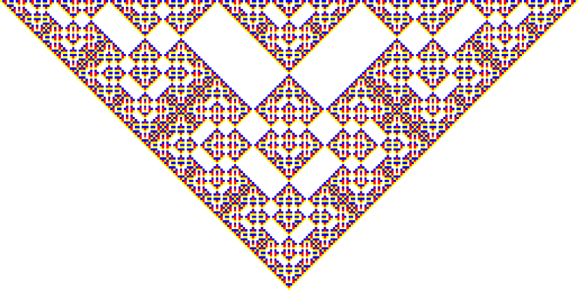
Figure 2: Time evolution of a fractal CSCA (20). Time increases upwards. The different colors illustrate the different Pauli matrices.

Nevertheless, we will state one short lemma, that we will need later on to prove the convergence of product states.

Lemma II.15.

If a CSCA t is fractal, so is ${\textbf{\emph{t}}}^{n}$ for $n\in\mathbb{N}$.

Proof.

We prove that ${\textbf{\emph{t}}}^{n}$ is fractal by showing that it can neither be periodic nor have gliders. Obviously, no power of t can be periodic if t is not periodic, so only the glider case remains. If ${\textbf{\emph{t}}}^{n}$ has minimal gliders $\xi$, $\bar{\xi}$ then by

$${\textbf{\emph{t}}}^{n}({\textbf{\emph{t}}}\xi)={\textbf{\emph{t}}}{\textbf{\emph{t}}}^{n}\xi=\lambda({\textbf{\emph{t}}}\xi)$$

${\textbf{\emph{t}}}\xi$ is also a glider for ${\textbf{\emph{t}}}^{n}$ with the same eigenvalue $\lambda$ and thus a multiple of $\xi$. Hence ${\textbf{\emph{t}}}\xi=\tilde{\lambda}\xi$ holds for a monomial $\tilde{\lambda}$. If $\tilde{\lambda}=1$ the automaton would be periodic by Proposition II.14 which is already ruled out. For $\tilde{\lambda}=u^{\pm n}$, which is the only other possibility, t has gliders. Thus for ${\textbf{\emph{t}}}^{n}$ to have gliders t has to have gliders. This is a contradiction to the assumption that t is fractal. So any power of a fractal CSCA is always fractal. ∎

III Invariant states and convergence

In this section we will consider different types of states on the spin chain and their evolution under CQCA action. Our focus lies on the search for invariant states and the convergence of other states towards invariant states. We consider special sets of states: product states, stabilizer states and quasifree states. Because CQCAs act in a translation-invariant manner, it is natural to look at translation-invariant states. We will therefore only consider those.

The only state that we know to be invariant for all CQCAs (and all QCAs) is the tracial state, which vanishes on all finite Pauli products except the identity and is defined as the limit of states that have the density operator $\frac{1}{2}\mathds{1}$ for each tensor factor. We strongly suspect this state to be the only invariant state for fractal CQCAs, but have no complete proof yet.

III.1 Invariant states for periodic CQCAs

It is obvious, that all states are periodic under the action of periodic CQCAs. Therefore a state is either invariant or does not converge at all. Finding invariant states for periodic automata is in general very easy. For example, if a CQCA satisfies $T^{p}=\mathds{1}$ for some finite $p\in\mathds{N}^{+}$, then all states of the type $\frac{1}{p}\sum_{n=1}^{p}\omega\circ T^{n}$ are invariant. Moreover, any invariant state is of this form, because for $\omega$ invariant $\omega=\frac{1}{p}\sum_{n=1}^{p}\omega\circ T^{n}$. Finding pure invariant states is more complicated. In Section III.3.1 we show, that for some period-two CQCAs pure invariant stabilizer states exist. For CQCAs without propagation there also exist invariant product states. Namely, if one Pauli matrix is left invariant by such a CQCA, then the state that gives expectation value one on this matrix and vanishes on the others is left invariant by this CQCA. A state with the same expectation value for all Pauli matrices is always left invariant by a non-propagating CQCA.

III.2 Invariance and convergence of product states for non-periodic automata

In this section we will only consider states which are translation-invariant product states with respect to single cell systems. They are of the form $\omega({\bf w}(\xi))=\prod_{i}\Phi({\bf w}(\xi_{i}))$, where $\Phi$ is a state on a single cell.

Proposition III.1.

For a glider CQCA $T$ there exist no translation-invariant product states that are T-invariant except the tracial state. All other translation-invariant product states weakly converge to $T$-invariant states

$$\omega_{\infty}=\lim_{n\to\infty}\omega\circ T^{n}.$$ (21)

with the following properties:

• $\omega_{\infty}({\bf w}(\xi))=1$, if ${\bf w}(\xi)=\mathds{1}$,

• $|\omega_{\infty}({\bf w}(\xi))|<1$, if ${\bf w}(\xi)$ is a product of gliders,

• $\omega_{\infty}({\bf w}(\xi))=0$ otherwise.

If $\Phi(\sigma_{j})=1$ for some $j$, then $\omega_{\infty}$ is the tracial state.

Proof.

First we prove the non-existence of invariant product states. A state is invariant if $\omega\circ T=\omega$, i.e., $\omega(TA)=\omega(A),\,\forall A\in\mathfrak{A}$ has to be fulfilled. We require the automaton to be non-periodic which implies a finite (non-zero) propagation, so at least two of the Pauli matrices are mapped to tensor products of at least three Pauli matrices. Thus for these two Pauli matrices ${\bf w}(\xi)$

$$\Phi({\bf w}(\xi)) = \omega({\bf w}(\xi))$$

$$= \omega(T{\bf w}(\xi))$$

$$= \prod_{i\in\mathcal{N}}\Phi({\bf w}(({\textbf{\emph{t}}}\xi)_{i}))$$

holds. For all Pauli matrices $\sigma_{i}$, $|\Phi(\sigma_{i})|\leq 1$. If $|\Phi(\sigma_{i})|=1$, then $\Phi(\sigma_{j})=0,\,\forall j\neq i$. Now lets assume that $\Phi(\sigma_{i})\neq 0$ for some $i$. The image of a single cell observable has to include at least two different types of Pauli matrices (different from the identity, e.g. $\sigma_{1}$ and $\sigma_{2}$). Else $\xi_{+}=0$ or $\xi_{-}=0$ or $\xi_{+}=\xi_{-}$, each case implying common divisors.

Let us consider the case when there exists a Pauli matrix which is not mapped to a tensor product. It can not be mapped to itself, because then by Proposition II.14 the automaton would be periodic. So it has to be mapped to another Pauli matrix which has to expand in the next step. Thus we only need to consider the case of expanding Pauli matrices. The image has to consist of more than one kind of Pauli matrices, so $|\Phi(\sigma_{i})|=1$ is ruled out as an invariant state. Moreover, the image can not contain the original Pauli matrix even once, because $\Phi(\sigma_{i_{k}})=(\Pi_{j\in\mathcal{N}\setminus k}\Phi(\sigma_{i_{j}}))\Phi(\sigma_{i_{k}})$ implies $|\Phi(\sigma_{i_{j}})|=1,\,\forall i_{j}$ which is already ruled out. So no Pauli matrix may occur in its own image, particularly not in the central position. If we only consider those central positions, we get a local automaton. It is an easy calculation to show, that all of these automata, which map no Pauli matrix onto itself have trace one. So the trace of our CQCA contains a constant which is a contradiction to the condition that it has gliders. So $\Phi(\sigma_{i})=0,\,i=1,2,3$ and the only invariant state is the one with the density matrix $\rho_{\Phi}=\frac{1}{2}\mathds{1}$, i.e., the tracial state.

In the following we consider the convergence properties of product states. Clearly, it suffices to establish the convergence of Pauli products. First, suppose that some $|\Phi(\sigma_{j})|=1$. Then, according to Lemma A.1, for all Pauli products different from $\mathds{1}$, and all times except at most one, the evolved product will contain a Pauli matrix different from $\sigma_{j}$, and hence will have zero expectation in $\omega\circ T^{n}$. Hence $\omega_{\infty}$ is the tracial state.

To treat the remaining cases, we hence assume from now on that $|\Phi(\sigma_{j})|\leq\lambda<1$ for all three $j$. Hence if some Pauli product has $k$ factors different from $\mathds{1}$, its expectation in $\omega$ is at most $\lambda^{k}$. So let $k(t)$ be the number of non-identity factors in the $t^{\rm th}$ iterate of some Pauli product. If $k(t)$ diverges, we have nothing to prove. So we may assume from now on that there is a constant $k_{max}<\infty$ such that $k(t)<k_{max}$ infinitely often. We focus on the subsequence for which this is the case.

If the overall length of the Pauli product (largest-smallest degree) remains finite, and since we have assumed the absence of periodic finite configurations, then we must have a glider for some power of $T$. As argued in the proof of Lemma II.15, this is also a glider for $T$. In fact, for any product of glider elements, the left going and the right going gliders will eventually be separated, and from that point onwards the $\omega$-expectation will not change anymore. Hence the limit does exist and will be some number of modulus $<1$.

Hence we need only consider the case that $k_{max}$ is finite, but the positions of non-identity Pauli factors get more and more spread out. This is only possible, if some Pauli products near the edges of the given product have a similar property: no sub-product which gets widely separated from the rest is allowed to develop configurations with unbounded $k_{max}$, because then the overall bound could not hold. Thus we again find bounded configurations with smaller $k_{max}$, which may again be smaller gliders, or split up even further. By downwards induction we just get a complete decomposition into gliders for any configuration with non-divergent $k_{max}$. This completes our proof. ∎

Proposition III.2.

Under the action of fractal CQCAs all product states converge to the tracial state.

Proof.

To show convergence for the fractal case, we need the results from Section II.2.3 and Appendix A.1. They state, that a tensor product with only one kind of Pauli matrices can occur only once in the history of a fractal CQCA and that the number of non-identity tensor factors grows unbounded. With the arguments used in the proof of Theorem III.1 this means that for fractal CQCAs any given product state converges to the state which gives zero expectation value for any non-trivial tensor products of Pauli operators, i.e., to the tracial state. ∎

III.3 Invariance and convergence of stabilizer states

In this chapter we consider pure translation-invariant stabilizer states. A stabilizer state is the common eigenstate of an abelian group of operators (usually tensor products of Pauli matrices) called the stabilizer group $\mathcal{S}$. For those not familiar with the stabilizer formalism we give a short example.

Example III.3.

The stabilizer group $\mathcal{S}=\langle\sigma_{1}\otimes\sigma_{1},\sigma_{3}\otimes\sigma_{3}\rangle$ stabilizes the Bell state $\psi=1/\sqrt{2}(\left|1,1\right>+\left|0,0\right>)$. We check this by applying the stabilizer generators to the state (normalization is omitted):

$$(\sigma_{1}\otimes\sigma_{1})\psi = (\sigma_{1}\otimes\sigma_{1})(\left|1\right>\otimes\left|1\right>)+(\sigma_{1}\otimes\sigma_{1})(\left|0\right>\otimes\left|0\right>)$$

$$= \left|0,0\right>+\left|1,1\right>=\psi$$

$$(\sigma_{3}\otimes\sigma_{3})\psi = (\sigma_{3}\otimes\sigma_{3})(\left|1\right>\otimes\left|1\right>)+(\sigma_{3}\otimes\sigma_{3})(\left|0\right>\otimes\left|0\right>)$$

$$= (-\left|1\right>)\otimes(-\left|1\right>)+\left|0\right>\otimes\left|0\right>$$

$$= (-1)^{2}\left|1,1\right>+\left|0,0\right>=\psi$$

$\lozenge$

Now we move on to translation-invariant stabilizer states. Consider the stabilizer group $\mathcal{S}=\langle{\bf w}(\hat{\tau}^{x}\xi),x\in\mathbb{Z}\rangle$ generated by the translates of a Pauli tensor product ${\bf w}(\xi)$, where $\hat{\tau}^{x}$ denotes the $x$-th power of the phase space translation. The unique state $\omega$ satisfying $\omega(A)=1$ for all $A\in\mathcal{S}$ is called the pure translation-invariant stabilizer state corresponding to the stabilizer $\mathcal{S}$ SchlingemannCQCA . In the following we will refer to the stabilizer group simply as “stabilizer”.

III.3.1 Invariance

Let us first search which CQCAs leave pure translation-invariant stabilizer states invariant.

Proposition III.4.

Only periodic CQCAs can leave pure translation-invariant stabilizer states invariant. For each such stabilizer state with stabilizer $\mathcal{S}=\langle{\bf w}(\hat{\tau}^{x}\xi),\,x\in\mathbb{Z}\rangle$ the CQCAs that leave the state invariant are periodic and form a group. The corresponding CSCAs are

$${\textbf{\emph{t}}}_{\xi}(a)=\left(\begin{array}[]{cc}1+a\xi_{+}\xi_{-}&a\xi_{+}^{2}\\ a\xi_{-}^{2}&1+a\xi_{+}\xi_{-}\end{array}\right),$$ (22)

for a centered palindrome $a$.

Proof.

The invariance condition for a stabilizer state with stabilizer $\mathcal{S}=\langle{\bf w}(\hat{\tau}^{x}\xi),\,x\in\mathbb{Z}\rangle$ is

$${\textbf{\emph{t}}}\xi=\alpha\xi,\,\alpha\in{\mathcal{P}}.$$

In SchlingemannCQCA it was proved that for every translation-invariant stabilizer state $\omega$ with stabilizer $\mathcal{S}=\langle{\bf w}(\hat{\tau}^{x}\xi),\,x\in\mathbb{Z}\rangle$ there exists a CQCA $B$, which maps ${\bf w}(0,1)$ to ${\bf w}(\xi)$. Thus the condition becomes

$${\textbf{\emph{t}}}{\bf b}\tbinom{0}{1}=\alpha{\bf b}\tbinom{0}{1}.$$

If we know automata that leave the “all spins up” state invariant, we can construct automata for arbitrary translation-invariant pure stabilizer states via

$$\begin{array}[]{crcl}&\phantom{\dbinom{0}{0}}{\textbf{\emph{t}}}\tbinom{0}{1}&=&\alpha\tbinom{0}{1}\\ \Leftrightarrow&\underbrace{{\bf b}{\textbf{\emph{t}}}{\bf b}^{-1}}_{{\textbf{\emph{t}}}_{\xi}}\underbrace{{\bf b}\tbinom{0}{1}}_{\xi}&=&\alpha{\bf b}\tbinom{0}{1}\\ \Leftrightarrow&{\textbf{\emph{t}}}_{\xi}\xi&=&\alpha\xi.\end{array}$$

The only type of CQCAs that leave the “all spins up” state invariant are the shear transformations, which are represented by matrices

$${\textbf{\emph{t}}}={\left(\begin{array}[]{cc}1&0\\ {a}&1\end{array}\right)}$$

with some palindrome $a$. A direct computation shows that the factor $\alpha$ has to be invertible. As we are in characteristic two and deal with centered automata, only $\alpha=1$ is possible. For a general translation-invariant stabilizer state the CQCAs that leave it invariant are represented by the CSCAs with matrices

$${\textbf{\emph{t}}}_{\xi}(a)=\left(\begin{array}[]{cc}1+a\xi_{+}\xi_{-}&a\xi_{+}^{2}\\ a\xi_{-}^{2}&1+a\xi_{+}\xi_{-}\end{array}\right).$$

The product of two such CQCAs also leaves the state invariant with ${\textbf{\emph{t}}}_{\xi}(a){\textbf{\emph{t}}}_{\xi}(b)={\textbf{\emph{t}}}_{\xi}(a+b)$. The inverse of each periodic CQCA is one of its powers, so it is also included in this set. We therefore have a group of period two CQCAs for each translation-invariant pure stabilizer state that leave this state invariant. ∎

III.3.2 Convergence

We now consider an arbitrary translation-invariant stabilizer state $\omega_{{\bf w}(\xi)}$ and the respective stabilizer $\mathcal{S}=\langle{\bf w}(\hat{\tau}^{x}\xi),\,x\in\mathbb{Z}\rangle$. There exists a CQCA $B$ satisfying $B({\bf w}(\xi))=\sigma_{3}$. We rewrite our state in terms of the $\sigma_{3}$-state

$$\omega_{{\bf w}(\xi)}=\omega_{\sigma_{3}}\circ B^{-1}$$ (23)

and use

$$\omega_{{\bf w}(\xi)}(T^{n}(\bigotimes\sigma_{i}))$$

$$= \omega_{\sigma_{3}}(B^{-1}T^{n}(\bigotimes\sigma_{i}))$$

$$= \omega_{\sigma_{3}}((B^{-1}TB)^{n}B^{-1}(\bigotimes\sigma_{i})).$$

$B^{-1}TB$ is also a CQCA of the same type (same trace) as $T$ and $B^{-1}(\bigotimes\sigma_{i})$ is a tensor product of Pauli matrices. $\omega_{\sigma_{3}}$ is a product state and thus converges according to Propositions III.1 and III.2 for glider and fractal CQCAs.

III.4 Stationary quasifree states and convergence of quasifree states for one-step glider CQCAs

In the previous sections we discussed stationary states and convergence of states under general CQCA actions. In this section we consider the particular glider CQCA $G$ which is represented by the CSCA

$${\textbf{\emph{g}}}=\left(\begin{array}[]{cc}1&u^{-1}+u\\ 1&u^{-1}+1+u\end{array}\right),$$ (24)

because for this CQCA we can obtain new types of stationary states and new convergence results by employing the Araki-Jordan-Wigner transformation. Using the Theorem for glider equivalence II.12 we can construct invariant states for all automata with gliders that move one step in space every timestep. According to this theorem for any speed-one glider CQCA $B$, there is a CQCA $A$ such that $B=AGA^{-1}$, and if $\omega$ is a $G$-invariant state, then $\omega\circ A^{-1}$ will be $B$-invariant.

III.4.1 Araki-Jordan-Wigner transformation

The Jordan-Wigner transformation is a way to map a finite spin-chain algebra $\mathcal{M}_{2}^{\otimes N}$ to the algebra of a finite fermion chain. This method has been extensively used in solid state physics LSM ; BMD ; BM . However, the method cannot be carried over directly to two-sided infinite chains. One has to introduce an additional infinite “tail-element” for the transformation to work. This extended transformation was introduced by Araki in his study of the two-sided infinite XY-chain araki-ajw , and it is sometimes referred to as the Araki-Jordan-Wigner construction.

The C^∗-algebra describing a two-sided infinite fermion chain is the algebra $\mathcal{F}$=CAR($\ell^{2}(\mathbb{Z})$), i.e., it is the C^∗-algebra generated by $\mathbbm{1}$ and and the annihilation and creation operators $\{c^{\phantom{*}}_{x}\}_{x\in\mathbb{Z}}$ and $\{c^{*}_{x}\}_{x\in\mathbb{Z}}$, satisfying the canonical anticommutation relations:

$$c^{\phantom{*}}_{x}c^{*}_{y}+c^{*}_{y}c^{\phantom{*}}_{x}=\delta_{x,y}\mathbbm{1},\quad\quad c^{\phantom{*}}_{x}c^{\phantom{*}}_{y}+c^{\phantom{*}}_{y}c^{\phantom{*}}_{x}=0.$$

The translation automorphism $\tau_{\mathcal{F}}$ on this algebra is defined by $\tau_{\mathcal{F}}(c_{x})=c_{x+1}$. $\mathcal{F}$ is isomorphic to the observable algebra $\mathfrak{A}$ of the spin chain, but there exist no isomorphism $\iota\colon\mathfrak{A}\to\mathcal{F}$ that satisfies the property $\iota\circ\tau=\tau_{\mathcal{F}}\circ\iota$. This intertwining property would be needed to derive the translation invariance of a state $\omega\circ\iota$ on $\mathfrak{A}$ from that of $\omega$ on $\mathcal{F}$. This problem can be circumvented by the Araki-Jordan-Wigner construction.

The ordinary Jordan-Wigner isomorphism between the $N$-site spin-chain algebra $M_{2}^{\otimes N}$ (generated by the finite number of Pauli matrices $\{\sigma_{1}^{x},\sigma_{2}^{x},\sigma_{3}^{x}\}_{x\in\{0,1,\ldots,N-1\}}$ ), and the $N$-site fermion-chain algebra (generated by $\{c_{x},\;c_{x}^{*}\}_{x\in\{0,1,\ldots,N-1\}}$), is given by

$$\iota^{N}_{JW}(\sigma_{1}^{x}) := \prod_{y=0}^{x-1}(2c_{y}^{\phantom{*}}c_{y}^{*}-\mathbbm{1})(c_{x}^{*}+c_{x}^{\phantom{*}}),$$

$$\iota^{N}_{JW}(\sigma_{2}^{x}) := \prod_{y=0}^{x-1}(2c_{y}^{\phantom{*}}c_{y}^{*}-\mathbbm{1})i(c_{x}^{*}-c_{x}^{\phantom{*}}),$$

$$\iota^{N}_{JW}(\sigma_{3}^{x}) := 2c_{x}^{\phantom{*}}c_{x}^{*}-\mathbbm{1}.$$

However, as we have mentioned, the Jordan-Wigner transformation cannot be generalized to be a translation-intertwining isomorphism between the two-sided infinite spin and fermion chains. In an informal way, one could say that an element of the form “$\prod_{y=-\infty}^{-1}(2c_{y}^{\phantom{*}}c_{y}^{*}-\mathbbm{1})$” would be needed in the definition of a “two-sided infinite chain Jordan-Wigner transformation”. However, $\mathcal{F}$ doesn’t contain such an element. The basic idea of the Araki-Jordan-Wigner construction araki-ajw is to extend the algebra $\mathcal{F}$ with such an infinite tail-element. More concretely, one defines the C^∗-algebra $\widetilde{\mathcal{F}}$ to be the extension of $\mathcal{F}$ by a self-adjoint unitary element $U$ satisfying:

$$Uc_{x}U=\begin{cases}\text{ }c_{x}&\text{if}\;\;x\geq 0\\ -c_{x}&\text{if}\;\;x<0\end{cases}.$$

Clearly, every element of $\widetilde{\mathcal{F}}$ can be uniquely written in the form $a+Ub$ with $a,b\in\mathcal{F}$, i.e. $\widetilde{\mathcal{F}}=\mathcal{F}+U\mathcal{F}$. One can extend the translation automorphism $\tau_{\mathcal{F}}$ to $\widetilde{\mathcal{F}}$ through the formula $\tilde{\tau}_{\mathcal{F}}(a+Ub):=\tau_{\mathcal{F}}(a)+U(2c_{0}c_{0}^{*}-\mathbbm{1})\tau_{\mathcal{F}}(b)$. Let us define the elements

$$A_{x}:=\begin{cases}\prod_{y=0}^{x-1}(2c_{y}^{\phantom{*}}c_{y}^{*}-\mathbbm{1})&\text{if }x>0\\ \mathbbm{1}&\text{if }x=0\\ \prod_{y=x}^{-1}(2c_{y}^{\phantom{*}}c_{y}^{*}-\mathbbm{1})&\text{if }x<0\end{cases},$$

and let us introduce the elements

$$\widehat{\sigma_{1}}^{x}:=UA_{x}(c_{x}^{*}+c_{x}^{\phantom{*}}),\quad\widehat{\sigma_{2}}^{x}:=UA_{x}i(c_{x}^{*}-c_{x}^{\phantom{*}}),\quad\widehat{\sigma_{3}}^{x}:=(2c_{x}^{\phantom{*}}c_{x}^{*}-\mathbbm{1}).$$ (25)

Denote by $\widehat{\mathcal{F}}$ the C^∗-subalgebra of $\widetilde{\mathcal{F}}$ which is generated by the elements of $\{\widehat{\sigma_{1}}^{x},\widehat{\sigma_{2}}^{x},\widehat{\sigma_{3}}^{x}\,|\,x\in\mathbb{Z}\}$. A direct computation shows that the elements defined in (25) having the same “spatial index” $x$ satisfy the Pauli-relations, while any two of these elements having two different spatial indices commute. Hence $\widehat{\mathcal{F}}$ and $\mathfrak{A}$ are isomorphic, and an isomorphism is given by the map $\Pi:\widehat{\mathcal{F}}\to\mathfrak{A}$, defined as

$$\Pi(\widehat{\sigma_{1}}^{x})=\sigma_{1}^{x}\,,\;\Pi(\widehat{\sigma_{2}}^{x})=\sigma_{2}^{x}\,,\;\Pi(\widehat{\sigma_{3}}^{x})=\sigma_{3}^{x}\,,\;\;\;\forall x\in\mathbb{Z}.$$

Moreover, if we denote by $\widehat{\tau}_{\mathcal{F}}$ the restriction of $\widetilde{\tau}_{\mathcal{F}}$ to $\widehat{\mathcal{F}}$ then

$$\tau\circ\Pi=\Pi\circ\widehat{\tau}_{\mathcal{F}},$$

i.e., $\Pi$ intertwines the translations of the two algebras.

Let $\omega$ be a translation-invariant state on the fermion-chain algebra $\mathcal{F}$. By defining $\widetilde{\omega}(a+Ub):=\omega(a)$ we get a translation-invariant state on $\widetilde{\mathcal{F}}$. Restricting this state to $\widehat{\mathcal{F}}$ we get a $\widehat{\tau}_{\mathcal{F}}$-invariant state $\widehat{\omega}$, and $\omega^{JW}=\widehat{\omega}\circ\Pi^{-1}$ will be a translation-invariant state on the quantum spin-chain. In this way we can transfer translation-invariant states from the fermion-chain to the spin-chain.

Any CQCA automorphism $T$ can naturally be transferred to an automorphism on $\widehat{\mathcal{F}}$ commuting with $\widehat{\tau}_{\mathcal{F}}$ by the definition $\widehat{T}:=\Pi\circ T\circ\Pi^{-1}$. In the case of the glider CQCA $G$ (24) we can do even more. The transferred automorphism $\widehat{G}$ (characterized by $\widehat{G}(\widehat{\sigma_{1}}^{x})=\widehat{\sigma_{2}}^{x}$, $\widehat{G}(\widehat{\sigma_{2}}^{x})=\widehat{\sigma_{2}}^{x-1}\widehat{\sigma_{1}}^{x}\widehat{\sigma_{2}}^{x+1}$) can also be extended to an automorphism $\widetilde{G}:\widetilde{F}\to\widetilde{F}$ in a translation-invariant way ($\widetilde{G}\circ\tilde{\tau}_{F}=\tilde{\tau}_{F}\circ\widetilde{G}$) with the following definition:

$$\widetilde{G}(U)=iU(c^{\phantom{*}}_{-1}+c^{*}_{-1})(c^{\phantom{*}}_{0}-c^{*}_{0}).$$

It is exactly this type of “translation-invariant extension property” that allows us to find stationary translation-invariant states of the glider CQCA by the Araki-Jordan-Wigner method.

Restricting the $\widetilde{G}$ automorphism to the fermion-chain subalgebra $\mathcal{F}\subset\widetilde{\mathcal{F}}$, we obtain the automorphism $G_{\mathcal{F}}$, which acts in the following way:

$$G_{\mathcal{F}}(c_{x})=\frac{1}{2}(c^{*}_{x-1}+c^{\phantom{*}}_{x-1}+c^{*}_{x+1}-c^{\phantom{*}}_{x+1}).$$

The automorphism $G_{\mathcal{F}}:\mathcal{F}\to\mathcal{F}$ takes an especially simple form in terms of majorana operators. These operators are defined as

$$m_{2x}:=i(c^{\phantom{*}}_{x}-c_{x}^{*}),\quad\quad m_{2x+1}:=c^{\phantom{*}}_{x}+c_{x}^{*},$$ (26)

for any $x\in\mathbb{Z}$, and they generate $\mathcal{F}$. The action of $G_{\mathcal{F}}$ on these operators is

$$G_{\mathcal{F}}(m_{2x})=m_{2x-2},\quad\quad\quad G_{\mathcal{F}}(m_{2x+1})=m_{2x+3}.$$

Clearly, if we find a state $\omega$ on $\mathcal{F}$ that is both $\tau_{\mathcal{F}}\,$- and $G_{\mathcal{F}}$-invariant, then the Araki-Jordan-Wigner transformed state $\omega^{JW}$ will be a $\tau$- and $G$-invariant state on the quantum spin-chain. In the next section, we will recall the definition of quasifree states on fermion-chains and then determine the translation- and $G_{\mathcal{F}}$-invariant quasifree states. In this way, using the Araki-Jordan-Wigner construction, we can obtain a whole class of translation- and $G$-invariant states on the spin-chain.

III.4.2 Stationary quasifree states

A state $\omega:\mathcal{F}\to\mathbb{C}$ is called quasifree if it vanishes on odd monomials of majorana operators

$$\omega(m_{x_{1}}\dots m_{x_{2n-1}})=0,$$

while on even monomials of majorana operators it factorizes in the following form:

$$\omega(m_{x_{1}}\dots m_{x_{2n}})=\sum\limits_{\pi}{\text{sgn}}(\pi)\prod\limits_{l=1}^{n}\omega(m_{x_{\pi(2l-1)}}m_{x_{\pi(2l)}}),$$

where the sum runs over all pairings of the set $\{1,2,\ldots,2n\}$, i.e., over all the $\pi$ permutations of the $2n$ elements which satisfy $\pi(2l-1)<\pi(2l)$ and $\pi(2l-1)<\pi(2l+1)$. Hence, if we assume that $x_{i}\neq x_{j}$ when $i\neq j$, then $\omega(m_{x_{1}}\ldots m_{x_{2}n})$ is simply the Pfaffian of the $2n\times 2n$ antisymmetric matrix $A_{i,j}:=\omega(m_{x_{i}}m_{x_{j}})$.

An automorphism $\alpha:\mathcal{F}\to\mathcal{F}$ that maps any majorana operator onto a linear combination of majorana operators is called a Bogoliubov automorphism araki . For any quasifree state $\omega$, the Bogoliubov transformed state $\omega^{\prime}:=\omega\circ\alpha$ will again be quasifree.

A quasifree state $\omega$ is translation-invariant, i.e. $\omega\circ\tau_{\mathcal{F}}=\omega$, iff $\omega(m_{x}m_{y})=\omega(m_{x+2}m_{y+2})$ for all $x,y\in\mathbb{Z}$. Translation-invariant quasifree states are characterized by a majorana two-point matrix which is a $2\times 2$-block Toeplitz matrix of the form (for a proof, see e.g. AB )

$$\begin{bmatrix}\omega(m_{2x}m_{2y})&\omega(m_{2x}m_{2y+1})\\ \omega(m_{2x+1}m_{2y})&\omega(m_{2x+1}m_{2y+1})\end{bmatrix}=\frac{1}{2\pi}\int_{-\pi}^{\pi}\begin{bmatrix}q_{1,1}^{(\omega)}(p)&q_{1,2}^{(\omega)}(p)\\ q_{2,1}^{(\omega)}(p)&q_{2,2}^{(\omega)}(p)\end{bmatrix}e^{-ip(x-y)}{\rm d}p,$$ (27)

where $q_{i,j}^{(\omega)}$ are $L^{\infty}([-\pi,\pi])$ functions, and the matrix function

$$Q^{(\omega)}(p)=\begin{bmatrix}q_{1,1}^{(\omega)}(p)&q_{1,2}^{(\omega)}(p)\\ q_{2,1}^{(\omega)}(p)&q_{2,2}^{(\omega)}(p)\end{bmatrix}\in L^{\infty}_{2\times 2}([-\pi,\pi])$$

satisfies

$$(Q^{(\omega)}(p))^{\dagger}=Q^{(\omega)}(p),\;\;Q^{(\omega)}(-p)=2\cdot\mathbbm{1}-(Q^{(\omega)}(p))^{T},\;\;0\leq Q^{(\omega)}(p)\leq 2\cdot\mathbbm{1}$$ (28)

almost everywhere (here $(Q^{(\omega)}(p))^{T}$ denotes the transpose of $Q^{(\omega)}(p)$). A translation-invariant quasifree state $\omega$ is pure iff for almost every $p$ the eigenvalues of $Q^{(\omega)}(p)$ are either $0$ or $2$. $Q^{(\omega)}(p)$ is called the symbol of the majorana two-point matrix $M^{\omega}_{x,y}=\omega(m_{x}m_{y})$.

Now we are ready to characterize the translation-invariant quasifree states that are stationary with respect to the time-evolution $G_{\mathcal{F}}$ (defined in the previous subsection).

Proposition III.5.

A translation-invariant quasifree state $\omega$ is invariant under the $G_{\mathcal{F}}$ automorphism iff the symbol of its majorana two-point matrix has the following form:

$$Q^{(\omega)}(p)=\begin{bmatrix}q_{1,1}^{(\omega)}(p)&0\\ 0&q_{2,2}^{(\omega)}(p)\end{bmatrix},$$

where $q_{1,1}^{(\omega)}$ and $q_{2,2}^{(\omega)}$ are real $L^{\infty}([-\pi,\pi])$ functions that take values between $0$ and $2$ (almost everywhere).

Proof.

The $G_{\mathcal{F}}$ automorphism acts on the majorana fermions as

$$G_{\mathcal{F}}(m_{2x})=m_{2x-2}\,,\;\;\;G_{\mathcal{F}}(m_{2x+1})=m_{2x+3}\;,$$

hence it is a Bogoliubov automorphism. Moreover, $G_{\mathcal{F}}$ commutes with the translations. Thus $\omega^{\prime}=\omega\circ G_{\mathcal{F}}$ will again be a translation-invariant quasifree state, and $\omega^{\prime}$ is equal to $\omega$ iff its majorana two-point matrix is the same as that of $\omega$. The majorana two-point function of $\omega^{\prime}$ is

$$\begin{bmatrix}\omega^{\prime}(m_{2x}m_{2y})&\omega^{\prime}(m_{2x}m_{2y+1})\\ \omega^{\prime}(m_{2x+1}m_{2y})&\omega^{\prime}(m_{2x+1}m_{2y+1})\end{bmatrix} = \begin{bmatrix}\omega(G_{\mathcal{F}}(m_{2x}m_{2y}))&\omega(G_{\mathcal{F}}(m_{2x}m_{2y+1}))\\ \omega(G_{\mathcal{F}}(m_{2x+1}m_{2y}))&\omega(G_{\mathcal{F}}(m_{2x+1}m_{2y+1}))\end{bmatrix}$$

$$= \begin{bmatrix}\omega(m_{2x-2}m_{2y-2})&\omega(m_{2x-2}m_{2y+3})\\ \omega(m_{2x+3}m_{2y-2})&\omega(m_{2x+3}m_{2y+3})\end{bmatrix}$$

$$= \begin{bmatrix}\omega(m_{2x}m_{2y})&\omega(m_{2x-2}m_{2y+3})\\ \omega(m_{2x+3}m_{2y-2})&\omega(m_{2x+1}m_{2y+1})\end{bmatrix},$$

where we have used that $\omega$ is $\tau_{\mathcal{F}}$-invariant, and that $\tau_{\mathcal{F}}(m_{x})=m_{x+2}$, which follows from the definition of the majorana operators (26). Comparing the majorana two-point functions, one can see that $\omega^{\prime}=\omega$ iff $\omega(m_{2x}m_{2y+1})=\omega(m_{2x-2}m_{2y+3})$ for any $x,y\in\mathbb{Z}$. From form (27) of the majorana two-point functions of translation-invariant quasifree states we know that there exists a $q^{(\omega)}_{1,2}$ $L^{\infty}([-\pi,\pi])$ function such that

$$\omega(m_{2x}m_{2y+1})=\frac{1}{2\pi}\int\limits_{-\pi}^{\pi}q_{1,2}^{(\omega)}(p)e^{-ip(x-y)}{\rm d}p.$$

The condition $\omega(m_{2x}m_{2y+1})=\omega(m_{2x-2}m_{2y+3})$, which should hold for all $x,y\in\mathbb{Z}$, means that

$$\frac{1}{2\pi}\int\limits_{-\pi}^{\pi}q_{1,2}^{(\omega)}(p)e^{-ip(x-y)}{\rm d}p-\frac{1}{2\pi}\int\limits_{-\pi}^{\pi}q_{1,2}^{(\omega)}(p)e^{-ip((x-1)-(y+1))}{\rm d}p$$

$$= \frac{1}{2\pi}\int\limits_{-\pi}^{\pi}q_{1,2}^{(\omega)}(p)(1-e^{2ip})e^{-ip(x-y)}{\rm d}p=0$$

must be satisfied. It is a well known theorem in functional analysis, that an $L^{\infty}([-\pi,\pi])$ function for which the Fourier transformation vanishes must be almost everywhere zero, hence $q_{1,2}^{(\omega)}(p)\cdot(1-e^{2ip})=0$, from which one concludes that $q_{1,2}^{(\omega)}(p)=0$. This means that for a $\tau_{\mathcal{F}}$- and $G_{\mathcal{F}}$-invariant state $\omega$ the symbol of the two-point majorana matrix has to be of the form

$$\begin{bmatrix}q_{1,1}^{(\omega)}(p)&0\\ 0&q_{2,2}^{(\omega)}(p)\end{bmatrix},$$

where $q^{(\omega)}_{1,1}$ and $q_{2,2}^{(\omega)}$ are $L^{\infty}([-\pi,\pi])$ functions, and according to (28) they also have to satisfy the inequalities $0\leq q^{(\omega)}_{1,1}(p)\leq 2$ and $0\leq q^{(\omega)}_{2,2}(p)\leq 2$ almost everywhere. Thus we have arrived at our proposition. ∎

Using the Araki-Jordan-Wigner transformation we can transfer such a $\tau_{\mathcal{F}}$- and $G_{\mathcal{F}}$-invariant quasifree state $\omega$ on $\mathcal{F}$ to a state $\omega^{JW}$ on the spin chain which is $\tau$-invariant and stationary with respect to the glider CQCA $G$.

III.4.3 Convergence of quasifree states

In this section we will show that under the repeated action of the $G_{\mathcal{F}}$ automorphism, any translation-invariant quasifree state will converge to one of the $G_{\mathcal{F}}$-invariant states specified in Proposition III.5.

Proposition III.6.

Let $\omega:\mathcal{F}\to\mathbb{C}$ be a translation-invariant quasifree state with a majorana two-point matrix that belongs to the symbol

$$Q^{(\omega)}(p)=\begin{bmatrix}q_{1,1}^{(\omega)}(p)&q_{1,2}^{(\omega)}(p)\\ q_{2,1}^{(\omega)}(p)&q_{2,2}^{(\omega)}(p)\end{bmatrix},$$

where $Q^{(\omega)}\in L^{\infty}_{2\times 2}([-\pi,\pi])$ satisfies the relations (28). The $n$ time-step evolved state is denoted by $\omega_{n}:=\omega\circ G_{\mathcal{F}}^{n}$. The pointwise limit $\omega_{\infty}(A):=\lim_{n\to\infty}\omega_{n}(A)$ exists for all $A\in\mathcal{F}$, and the function $\omega_{\infty}:\mathcal{F}\to\mathbb{C}$ defined in this way will be a translation-invariant quasifree state with a majorana two-point matrix that belongs to the following symbol

$$Q^{\left(\omega_{\infty}\right)}(p)=\begin{bmatrix}q_{1,1}^{(\omega)}(p)&0\\ 0&q_{2,2}^{(\omega)}(p)\end{bmatrix}.$$

Proof.

In the proof of Proposition III.5 we showed that if $\omega$ is a translation-invariant quasifree state, then $\omega_{2}=\omega\circ G_{\mathcal{F}}$ will also be such a state. By induction it follows that $\omega_{n}$ is also a translation-invariant quasifree state for any $n\in\mathbb{N}^{+}$. Hence for an arbitrary odd monomial of majorana operators $\omega_{n}(m_{x_{1}}m_{x_{2}}\cdots m_{x_{2N+1}})=0$, and the limit $\omega(m_{x_{1}}m_{x_{2}}\cdots m_{x_{2N+1}}):=\lim_{n\to\infty}\omega_{n}(m_{x_{1}}m_{x_{2}}\cdots m_{x_{2N+1}})$ exists and is zero.

Next, we prove the pointwise convergence of the majorana two-point matrix. The majorana two-point matrix of $\omega_{n}$ is

$$\begin{bmatrix}\omega_{n}(m_{2x}m_{2y})&\omega_{n}(m_{2x}m_{2y+1})\\ \omega_{n}(m_{2x+1}m_{2y})&\omega_{n}(m_{2x+1}m_{2y+1})\end{bmatrix} = \begin{bmatrix}\omega(G_{\mathcal{F}}^{n}(m_{2x}m_{2y}))&\omega(G_{\mathcal{F}}^{n}(m_{2x}m_{2y+1}))\\ \omega(G_{\mathcal{F}}^{n}(m_{2x+1}m_{2y}))&\omega(G_{\mathcal{F}}^{n}(m_{2x+1}m_{2y+1}))\end{bmatrix}$$

$$= \begin{bmatrix}\omega(m_{2x-2n}m_{2y-2n})&\omega(m_{2x-2n}m_{2y+1+2n})\\ \omega(m_{2x+1+2n}m_{2y-2n})&\omega(m_{2x+1+2n}m_{2y+1+2n})\end{bmatrix}$$

$$= \begin{bmatrix}\omega(m_{2x}m_{2y})&\omega(m_{2x-2n}m_{2y+1+2n})\\ \omega(m_{2x+1+2n}m_{2y-2n})&\omega(m_{2x+1}m_{2y+1})\end{bmatrix},$$

this means that the symbol $Q^{\left(\omega_{n}\right)}$ is given by

$$Q^{\left(\omega_{n}\right)}(p)=\begin{bmatrix}q_{1,1}^{(\omega)}(p)&q_{1,2}^{(\omega)}(p)e^{2inp}\\ q_{2,1}^{(\omega)}(p)e^{-2inp}&q_{2,2}^{(\omega)}(p)\end{bmatrix}.$$

The limits of elements of the two-point majorana matrix are:

$$\begin{bmatrix}\omega_{\infty}(m_{2x}m_{2y})&\omega_{\infty}(m_{2x}m_{2y+1})\\ \omega_{\infty}(m_{2x+1}m_{2y})&\omega_{\infty}(m_{2x+1}m_{2y+1})\end{bmatrix}$$ (29)

$$= \begin{bmatrix}\lim\limits_{n\to\infty}\omega_{n}(m_{2x}m_{2y})&\lim\limits_{n\to\infty}\omega_{n}(m_{2x}m_{2y+1})\\ \lim\limits_{n\to\infty}\omega_{n}(m_{2x+1}m_{2y})&\lim\limits_{n\to\infty}\omega_{n}(m_{2x+1}m_{2y+1})\end{bmatrix}$$

$$= \frac{1}{2\pi}\begin{bmatrix}\lim\limits_{n\to\infty}\int_{-\pi}^{\pi}q_{1,1}^{(\omega)}(p)e^{-i(x-y)p}{\rm d}p&\lim\limits_{n\to\infty}\int_{-\pi}^{\pi}q_{1,2}^{(\omega)}(p)e^{-i(x-y-2n)p}{\rm d}p\\ \lim\limits_{n\to\infty}\int_{-\pi}^{\pi}q_{2,1}^{(\omega)}(p)e^{-i(x-y+2n)p}{\rm d}p&\lim\limits_{n\to\infty}\int_{-\pi}^{\pi}q_{2,2}^{(\omega)}(p)e^{-i(x-y)p}{\rm d}p\end{bmatrix}$$

$$= \frac{1}{2\pi}\int_{-\pi}^{\pi}\begin{bmatrix}q_{1,1}^{(\omega)}(p)&0\\ 0&q_{2,2}^{(\omega)}(p)\end{bmatrix}e^{-ip(x-y)}{\rm d}p,$$

where we have used the Riemann-Lebesgue lemma, which states that for any integrable function $f$ defined on the interval $[a,b]$:

$$\lim_{z\to\pm\infty}\int\limits_{a}^{b}f(x)e^{izx}dx=0.$$

For an arbitrary even monomial of majorana operators the convergence can be proved by:

$$\omega_{\infty}(m_{x_{1}}m_{x_{2}}\cdots m_{x_{2N+1}}) = \lim_{n\to\infty}\omega_{n}(m_{x_{1}}m_{x_{2}}\cdots m_{x_{2N+1}})$$ (30)

$$= \lim_{n\to\infty}\sum\limits_{\pi}{\text{sgn}}(\pi)\prod\limits_{l=1}^{N}\omega_{n}(m_{x_{\pi(2l-1)}}m_{x_{\pi(2l)}})=$$

$$= \sum\limits_{\pi}{\text{sgn}}(\pi)\prod\limits_{l=1}^{N}\left[\lim_{n\to\infty}\omega_{n}(m_{x_{\pi(2l-1)}}m_{x_{\pi(2l)}})\right]=$$

$$= \prod\limits_{l=1}^{N}\omega_{\infty}(m_{x_{\pi(2l-1)}}m_{x_{\pi(2l)}}).$$

Since the finite linear combinations of majorana operators form a norm-dense subset in $\mathcal{F}$ the limit $\lim_{n\to\infty}\omega_{n}(f)$ must exist for any $f\in\mathcal{F}$ due to the uniform boundedness of the states in the sequence, and hence we have obtained with this pointwise limit a linear functional $\omega_{\infty}:\mathcal{F}\to\mathbb{R}$. Moreover, $\omega_{\infty}$ is uniquely determined by the values it takes on monomials of majorana operators, and since the equations (29), (30) are satisfied $\omega_{\infty}$ can only be the quasifree state for which the symbol of the majorana two-point function is given by (29) . ∎

It is worth mentioning that although a pure quasifree state will, of course, stay pure for any time $t$, taking the weak, i.e. pointwise, limit of the states when $t\to\infty$ one obtains a mixed state (if the original state was not $G$-invariant). In quantum many body physics such relaxation from a pure to mixed states has been studied in a quite different setting, namely how certain time averages of pure states that evolve under a Hamiltonian dynamics can be described by mixed states CDEO . It would be interesting to look at such weak limits when $t\to\infty$ also for Hamiltonian evolution (for systems with infinite degrees of freedom), and to look at the connection between these two approaches.

Finally we have to point out, that the results of this section using the AJW transformation can generally not be transferred to other CQCAs than the glider CQCA $G$, because most CQCAs don’t have the form of Bogoliubov transformations on the CAR-Algebra. Automata with neighborhoods larger than nearest neighbors can map creation and annihilation operators to products of these on the CAR-algebra and are thus in general not Bogoliubov transformations. (An obvious exception are powers of $G$.) All automata, that don’t leave at least one Pauli matrix locally invariant don’t allow for a tail element that is left invariant under the transformed CQCA. These automata are characterized by a constant in their trace polynomial. In conclusion, only nearest neighbor automata without a constant on the trace, i.e. some glider and period two automata and their powers, can be transferred to Bogoliubov transformations on the CAR-algebra. For more details see Uphoff2008 .

IV Entanglement generation

In this section we investigate the entanglement generation properties of CQCAs. First we derive general bounds for the entanglement generation of arbitrary QCAs on the spin-chain both in a translation-invariant and a non-translation-invariant setting. Then we investigate CQCAs acting on stabilizer and quasifree states. We find that the entanglement generation is linear in time, similarly to the case of Hamiltonian time evolutions CC .

IV.1 General bounds on the entanglement generation of QCA

In this section we derive general bounds on the evolution of the entanglement of a finite number of consecutive spins with the rest of the chain under the action of a localized automorphism (e.g. a QCA). We will only consider the case when the whole chain is in a pure state. In this case the proper measure of entanglement is given by the von Neumann entropy

$$S=-\rm{Tr}\,\rho_{S}\log_{2}\rho_{S},$$

where $\rho_{S}$ is the reduced density matrix of the finite segment of spins.

IV.1.1 The non-translation-invariant case

Theorem IV.1.

Consider the observable algebra of an infinite chain of $d$-level systems

$$\mathfrak{A}^{(d)}:=\bigotimes^{+\infty}_{i=-\infty}\mathfrak{A}_{i}^{(d)},\;\;\mathfrak{A}_{i}^{(d)}\cong M_{d},$$

and an automorphism $T:\mathfrak{A}^{(d)}\to\mathfrak{A}^{(d)}$. Let us introduce the notation: $\mathfrak{A}_{[m_{1},m_{2}]}^{(d)}:=\bigotimes^{m_{2}}_{k=m_{1}}\mathfrak{A}_{k}^{(d)}$. Suppose that $T$ satisfies the locality condition

$$T(\mathfrak{A}_{[k_{1},k_{2}]}^{(d)})\subset\mathfrak{A}_{[l_{1},l_{2}]}^{(d)}\;,$$

for some fixed integers $k_{1},k_{2},l_{1},l_{2}$, with $l_{1}\leq k_{1}$ and $k_{2}\leq l_{2}$.

Let $\omega$ be a state on the spin-chain $\mathfrak{A}^{(d)}$, and let us define the $T$-evolved state as $\omega^{\prime}:=\omega\circ T$. The restrictions of these states to a subalgebra $\mathfrak{A}_{[m_{1},m_{2}]}^{(d)}$ will be denoted by $\omega_{[m_{1},m_{2}]}$ and $\omega^{\prime}_{[m_{1},m_{2}]}$, respectively. Then the following bounds hold for the von Neumann entropies of the restricted states:

$$S(\omega_{[k_{1},k_{2}]})-2n\log_{2}d\leq S(\omega^{\prime}_{[k_{1},k_{2}]})\leq S(\omega_{[k_{1},k_{2}]})+2n\log_{2}d,$$ (31)

where $n=l_{2}-l_{1}-k_{2}+k_{1}$. Moreover, these bounds are sharp.

Proof.

Restricting the automorphism $T$ to the subsubalgebra $\mathfrak{A}_{[k_{1},k_{2}]}^{(d)}$, we get a monomorphism $T_{[k_{1},k_{2}]}:\mathfrak{A}_{[k_{1},k_{2}]}^{(d)}\to\mathfrak{A}_{[l_{1},l_{2}]}^{(d)}$. This monomorphism can be extended to an automorphism $\widetilde{T}:\mathfrak{A}_{[l_{1},l_{2}]}^{(d)}\to\mathfrak{A}_{[l_{1},l_{2}]}^{(d)}$. Let us introduce the following state on $\mathfrak{A}_{[l_{1},l_{2}]}$:

$$\widetilde{\omega}^{\prime}([l_{1},l_{2}]):=\omega_{[l_{1},l_{2}]}\circ\widetilde{T}.$$

From this construction it immediately follows that $\widetilde{\omega}^{\prime}([l_{1},l_{2}])_{[k_{1},k_{2}]}=\omega^{\prime}_{[k_{1},k_{2}]}$. Moreover, since $\widetilde{\omega^{\prime}}([l_{1},l_{2}]))$ and $\omega_{[l_{1},l_{2}]}$ are connected by an automorphism their von Neumann entropies are equal: $S(\widetilde{\omega}^{\prime}([l_{1},l_{2}]))=S(\omega_{[l_{1},l_{2}]})$.

We will prove the bounds (31) using the subadditivity of the von Neumann entropy. The subchain $\mathfrak{A}_{[l_{1},l_{2}]}^{(d)}$ can be divided as $\mathfrak{A}_{[l_{1},l_{2}]}^{(d)}=\mathfrak{A}_{[k_{1},k_{2}]}^{(d)}\otimes\mathfrak{A}_{rest}^{(d)}$, where $\mathfrak{A}_{rest}^{(d)}$ is isomorphic to the algebra of $d^{n}\times d^{n}$ matrices, hence the maximal entropy of a state defined on $\mathfrak{A}_{rest}^{(d)}$ is $n\log_{2}d$. The triangle inequality and the subadditivity theorem give the following inequalities:

$$S(\omega_{[k_{1},k_{2}]})-n\log_{2}d\leq S(\omega_{[l_{1},l_{2}]}) \leq S(\omega_{[k_{1},k_{2}]})+n\log_{2}d$$

$$S(\omega^{\prime}_{[k_{1},k_{2}]})-n\log_{2}d\leq S(\widetilde{\omega}^{\prime}({[l_{1},l_{2}]})) \leq S(\omega^{\prime}_{[k_{1},k_{2}]})+n\log_{2}d$$

Now, using that $S(\omega_{[l_{1},l_{2}]})=S(\widetilde{\omega}^{\prime}({[l_{1},l_{2}]}))$ we immediately obtain the bounds (31).

The sharpness of the inequalities follows if we consider a state on the spin-chain where the sites at $2i$ are maximally entangled with the sites at $2i+1$ and we consider the translation $\tau$ which just shifts all one-cell algebras by one cell to the right as our time-evolution. Then $k_{2}-k_{1}=2$ and $l_{2}-l_{1}=3$, and we get $n=l_{2}-l_{1}-k_{2}+k_{1}=1$. Now, restricting this state to the subalgebra $\mathfrak{A}_{2i,2i+3}^{(d)}$ the entropy of the restriction is zero. However, the entropy of this restriction after the time evolution will be $2\log_{2}d$, since the two sites at the border will be maximally entangled with sites outside the considered region. Let us note, that in some sense we broke the translation-invariance only minimally, since the considered state is invariant under the square of the translations $\tau^{2}$.

In the above example the generated entanglement is destroyed in the next step, so the bound is only saturated for one time step. But a slightly more involved example shows, that the bound can be saturated for arbitrarily many timesteps:

Let again $T$ be the translation automorphism on $\mathfrak{A}^{(d)}$, and let us consider the state on a spin-chain which is defined as the direct product of totally mixed states between the lattice site at $i$ and the lattice site at $-i+1$ for all $i$. So in this state the lattice site at $1$ is fully entangled with the lattice site at $0$, the lattice site at $2$ is fully entangled with the lattice site at $-1$, and so on. Now, we will consider subsystems of arbitrary length $k=k_{2}-k_{1}$. If $k$ is even, $k=2j$, then the subsystem we consider is the interval $[-j+1,j]$. Its original entropy is $0$, and the entropy grows linearly during the time-evolution saturating our linear bound until it reaches the maximal entropy it can obtain, namely $k\log_{2}d$. After this it stays constant. If $k$ is odd, $k=2j+1$, we consider the interval $[-j,j]$ as our subsystem. The original entropy of the subsystem is $\log_{2}d$, and the entropy grows linearly and saturates our bound until it reaches $(2j+1)\log_{2}d$, then it stays constant. ∎

IV.1.2 The translation-invariant case

In the previous subsection it was shown that the bounds (31) on entanglement generation are sharp in the general case. However, considering translation-invariant states and QCA automorphism, i.e., automorphisms that commute with the translations, we can sharpen these bounds further.

Theorem IV.2.

Consider the observable algebra of an infinite chain of $d$-level systems

$$\mathfrak{A}^{(d)}:=\bigotimes^{+\infty}_{i=-\infty}\mathfrak{A}_{i}^{(d)},\;\;\mathfrak{A}_{i}^{(d)}\cong M_{d},$$

and a QCA automorphism $T$ acting on $\mathfrak{A}^{(d)}$ having a neighborhood of $n$ “extra cells”, i.e., $T$ is an automorphism satisfying

$$T(\mathfrak{A}_{i})^{(d)}\subset\mathfrak{A}_{i-n_{1}}^{(d)}\otimes\mathfrak{A}_{i-n_{1}+1}^{(d)}\otimes\dots\otimes\mathfrak{A}_{i+n_{2}-1}^{(d)}\otimes\mathfrak{A}_{i+n_{2}}^{(d)}\;,\;\;\;\;T\circ\tau=\tau\circ T,$$ (32)

where $i\in\mathbb{Z}$, $\tau$ is the translation automorphism on $\mathfrak{A}^{(d)}$, and $n_{1}$ and $n_{2}$ are integers satisfying $n_{1}+n_{2}=n\geq 0$.

Let $\omega$ be a translation-invariant state on the spin-chain, and let us define the time-evolved state (at time $t\in\mathbb{N}$) as $\omega(t):=\omega\circ T^{t}$. The von Neumann entropy $S_{L}(t)$ of the restriction of $\omega(t)$ to $L$ consecutive qubits can be bounded in the following way:

$$S_{L}(0)-nt\log_{2}d\leq S_{L}(t)\leq S_{L}(0)+nt\log_{2}d.$$ (33)

Moreover, these bounds are sharp for $d=2$.

Proof.

Since the state $\omega$ is translation invariant and $T$ commutes with the translations, the “entropy production” is the same for the automorphisms $T$ and $T\circ\tau^{k}$ ($k\in\mathbb{Z}$), hence we can assume without loss of generality that in Eq. (32) $n_{1},n_{2}\geq 0$.

Let us denote the restriction of a state $\varphi:\mathfrak{A}^{(d)}\to\mathbb{C}$ to $\mathfrak{A}_{[m_{1},m_{2}]}^{(d)}=\bigotimes^{m_{2}}_{k=m_{1}}\mathfrak{A}_{k}^{(d)}$ by $\varphi_{[m_{1},m_{2}]}$. Consider the subalgebra $\mathfrak{A}_{[0,L-1]}^{(d)}$ of $\mathfrak{A}^{(d)}$, which corresponds to $L$ qubits. Restricting the automorphism $T$ to this subalgebra, we get a monomorphism $T_{L}:\mathfrak{A}_{[0,L-1]}^{(d)}\to\mathfrak{A}_{[-n_{1},L-1+n_{2}]}^{(d)}$. We will also consider the inverse automorphism $T^{-1}$, and restrict $T^{-1}$ to a monomorphism $(T^{-1})_{L}:\mathfrak{A}_{[0,L-1]}^{(d)}\to\mathfrak{A}_{[-n_{2},L-1+n_{1}]}^{(d)}$.. The monomorphism $(T^{-1})_{L}$ can be extended to an automorphism $\widetilde{T}^{-1}_{L}:\mathfrak{A}_{[-n_{2},L-1+n_{1}]}^{(d)}\to\mathfrak{A}_{[-n_{2},L-1+n_{1}]}^{(d)}$.

Let $\omega$ be a translation-invariant state on $\mathfrak{A}^{(d)}$, then $\omega(1):=\omega\circ T$ will be translation-invariant, too. Let us also define the following state on $\mathfrak{A}_{[-n_{2},L-1+n_{1}]}^{(d)}$

$$\widetilde{\omega}([-n_{2},L-1+n_{1}]):=\omega(1)_{[-n_{2},L-1+n_{1}]}\circ\widetilde{T}^{-1}_{L}.$$

The von Neumann entropy of $\widetilde{\omega}([-n_{2},L-1+n_{1}])$ and $\omega(1)_{[-n_{2},L-1+n_{1}]}$ are the same (since they are connected by an automorphism), and it follows from the definition of $\widetilde{T}^{-1}_{L}$ that $\widetilde{\omega}([-n_{2},L-1+n_{1}])_{[0,L-1]}=\omega_{[0,L-1]}$.

Now, from the strong subadditivity of the von Neumann entropy it follows that for a translation-invariant state $\omega$ $S(\omega_{[m_{1},m_{2}]})\geq S(\omega_{[k_{1},k_{2}]})$ if $m_{2}-m_{1}\geq k_{2}-k_{1}$ fannesbuch , hence

$$S_{L}(1)=S(\omega(1)_{[0,L-1]})\leq S(\omega(1)_{[-n_{2},L-1+n_{1}]}).$$ (34)

On the other hand, using the subadditivity of the entropy for the state $\widetilde{\omega}([-n_{2},L-1+n_{1}])$ (dividing the observable algebra of the subchain $[-n_{2},n_{1}]$ as: $\mathfrak{A}_{[-n_{2},L-1+n_{1}]}^{(d)}=\mathfrak{A}_{[0,L-1]}^{(d)}\otimes(\mathfrak{A}_{[-n_{2},-1]}^{(d)}\otimes\mathfrak{A}_{[L,L-1+n_{1}]}^{(d)}$)), we get:

$$S_{L}(\widetilde{\omega}([-n_{2},L-1+n_{1}]))\leq S_{L}(\widetilde{\omega}([-n_{2},L-1+n_{1}])_{[0,L-1]})+(n_{1}+n_{2})\log_{2}d=S_{L}(0)+n\log_{2}d$$ (35)

Combing the fact that $S(\omega(1)_{[-n_{2},L-1+n_{1}]})=S(\widetilde{\omega}([-n_{2},L-1+n_{1}]))$ with the inequalities (34) and (35) we arrive at the $S(1)\leq S(0)+n\log_{2}d$. By simple induction we obtain the desired upper bound:

$$S_{L}(t)\leq S_{L}(0)+nt\log_{2}d.$$

The lower bound in (33) can simply be obtained by ”reversing the time arrow”: suppose that for a QCA automorphism $T$ this lower bound does not hold, this would mean that for the QCA $T^{-1}$ the upper bound wouldn’t hold, which is a contradiction as we proved the upper bound just now.

The sharpness of the inequalities for $d=2$ follows from the study of of Clifford QCAs acting on the “all spin up state” in Section IV.2. ∎

IV.2 Entanglement generation starting from translation-invariant stabilizer states

In this section we will consider the entanglement generation of CQCA acting on translation-invariant pure stabilizer states. We will first calculate the bipartite entanglement in a general translation-invariant pure stabilizer state. Using this result we will present a proof of asymptotically linear growth of entanglement for non-periodic CQCAs.

For every translation-invariant stabilizer state $\omega$ with stabilizer $\mathcal{S}=\langle{\bf w}(\hat{\tau}^{x}\xi),\,x\in\mathbb{Z}\rangle$ there exists a CQCA $T$ which maps ${\bf w}(0,1)$ to ${\bf w}(\xi)$. Each $\mathcal{S}=\langle{\bf w}(\hat{\tau}^{x}\xi),\,x\in\mathbb{Z}\rangle$ defines a unique translation-invariant stabilizer state if and only if $\xi$ is reflection invariant and $\gcd(\xi_{+},\xi_{-})=1$ SchlingemannCQCA . The image of a one-site Pauli matrix under the action of a CQCA $B$ is always of this form. The study of the entanglement generation of CQCAs acting on initially unentangled stabilizer product states is thus equivalent to the study of the entanglement properties of translation-invariant stabilizer states.

There are several results on the entanglement entropy for stabilizer states in the literature, the most general example would be the formalism developed in Fattal2004 . One case considered is a bipartite split of the state $\omega_{AB}$ with respect to the subsystems $A$ and $B$. The set of stabilizers $\mathcal{S}$ then splits up into three sets. $\mathcal{S}_{A}$ and $\mathcal{S}_{B}$ are the local stabilizers, which act non-trivially only on part $A$ resp. $B$. The third set $\mathcal{S}_{AB}$ accounts for correlations between the subsystems. It is defined as follows:

Definition IV.3.

The correlation subgroup $\mathcal{S}_{AB}$ for a bipartite stabilizer state is generated by all stabilizer generators that have support on both parts of the system.

$\mathcal{S}_{A}$ and $\mathcal{S}_{B}$ together form the so called local subgroup. The correlation subgroup $\mathcal{S}_{AB}$ can be brought into a form where it consists of pairs of stabilizers whose projections on $A$ (and $B$) anticommute, but commute with all elements of other pairs and the local subgroup. The entanglement or von Neumann entropy of such a stabilizer state is

$$E(\omega_{AB})=\frac{1}{2}|\mathcal{S}_{AB}|,$$ (36)

if $\omega_{AB}$ is a pure state, where $|\mathcal{S}_{AB}|$ is the size of the minimal generating set of $\mathcal{S}_{AB}$.

Unfortunately, in Fattal2004 only finitely many qubits are considered. The proof of (36) relies heavily on this fact. However, there is a different approach to the bipartite entanglement in stabilizer states which we use to extend this result to infinitely many qubits.

In our approach we make use of the phase space description of stabilizer states introduced in SchlingemannCQCA . A stabilizer state is fixed by a set of defining commuting Pauli products. In the phase space description commutation relations are encoded in the symplectic form $\sigma(\xi,\eta)$. If $[{\bf w}(\xi),{\bf w}(\eta)]=0$ we have $\sigma(\xi,\eta)=0$. Thus abelian algebras of Weyl operators (Pauli products) correspond to subspaces on which the symplectic form vanishes. Those subspaces are called isotropic subspaces. If for an isotropic subspace ${\mathcal{I}}$ $\sigma(\eta,\xi)=0$, $\forall\xi\in{\mathcal{I}}$ implies $\eta\in{\mathcal{I}}$, we call ${\mathcal{I}}$ maximally isotropic. Maximally isotropic subspaces correspond to maximally abelian algebras. In SchlingemannCQCA it was shown that the above condition on $\xi$ (reflection invariance and $\gcd(\xi_{+},\xi_{-})=1$) is equivalent to the condition that ${\mathcal{P}}\xi$ is a maximally isotropic subspace. ${\mathcal{P}}\xi$ denotes the space generated by the products of $\xi$ and all elements of ${\mathcal{P}}$. We have $\langle{\bf w}(\eta),\eta\in{\mathcal{P}}\xi\rangle=\langle{\bf w}(\hat{\tau}^{x}\xi),\,x\in\mathbb{Z}\rangle=\mathcal{S}$. ${\mathcal{P}}\xi$ is the phase space of the stabilizer group $\mathcal{S}$. By $({\mathcal{P}}\xi)_{A}$ etc. we denote the phase spaces of $\mathcal{S}_{A}$ etc.

Theorem IV.4.

The number of maximally entangled qubit pairs in a pure translation invariant stabilizer state stabilized by $\mathcal{S}=\langle{\bf w}(\hat{\tau}^{x}\xi),\,x\in\mathbb{Z}\rangle$ on a bipartite spin-chain is the number of pairs $\eta^{i},\,\zeta^{i}\in({\mathcal{P}}\xi)_{AB}$ with $\sigma_{A}(\eta^{i},\zeta^{j})=\delta_{ij}$, $\sigma(\eta^{i}_{A},\eta^{j}_{A})=\sigma(\zeta^{i},\zeta^{j})=0$, $\sigma(\eta^{i}_{A},\mu)=\sigma(\eta^{i},\mu)=0,\,\forall\mu\in({\mathcal{P}}\xi)_{A}$, and $\sigma(\zeta_{A}^{i},\mu)=\sigma(\zeta^{i},\mu)=0,\,\forall\mu\in({\mathcal{P}}\xi)_{A}$. where $\eta_{A}$, $\zeta_{A}$ denote the restriction of the phase space vectors to subsystem $A$ completed with $0$ on $B$ so we can use the the symplectic form $\sigma$ of the whole chain.

Proof.

If we restrict the stabilizer to subsystem $A$ (or $B$) it is in general not translation invariant any more. Therefore the corresponding subspace is not maximally isotropic. The restricted state is not a pure translation invariant stabilizer state. However the uncut stabilizer operators in $\mathcal{S}_{A}$ stabilize a subspace of the statespace. The elements of the correlation subgroup $\mathcal{S}_{AB}$ which is generated by the cut stabilizer generators map this subspace onto itself because they commute with the elements of $\mathcal{S}_{A}$. From the theory of quantum error correction Gottesman1997 we know that a pair of operators leaving a stabilized subspace invariant can be used to encode a logical qubit if the operators fulfill the same commutation relations as $\sigma_{1}$ and $\sigma_{3}$. As the restrictions of the elements of $\mathcal{S}_{AB}$ don’t have to commute such pairs of operators can exist. In the phase space description this means, that we have to find $\eta,\,\zeta\in({\mathcal{P}}\xi)_{AB}$ with $\sigma(\eta_{A},\zeta_{A})=1$, $\sigma(\eta_{A},\mu_{A})=\sigma(\eta,\mu)=0,\,\forall\mu\in({\mathcal{P}}\xi)_{A}$, and $\sigma(\zeta_{A},\mu_{A})=\sigma(\zeta,\mu)=0,\,\forall\mu\in({\mathcal{P}}\xi)_{A}$. Several such pairs encode several qubits. Of course the operators from different pairs have to commute. Thus the qubits are encoded by pairs of operators $(\bar{\sigma}_{1}^{i},\bar{\sigma}_{3}^{i})=({\bf w}(\eta^{i}),{\bf w}(\zeta^{i}))$ whose phase space vectors fulfill $\sigma_{A}(\eta^{i},\zeta^{j})=\delta_{ij}$, $\sigma(\eta^{i}_{A},\eta^{j}_{A})=\sigma(\zeta^{i},\zeta^{j})=0$, $\sigma(\eta^{i}_{A},\mu)=\sigma(\eta^{i},\mu)=0,\,\forall\mu\in({\mathcal{P}}\xi)_{A}$, and $\sigma(\zeta_{A}^{i},\mu)=\sigma(\zeta^{i},\mu)=0,\,\forall\mu\in({\mathcal{P}}\xi)_{A}$. As we have $\sigma(\eta_{A},\zeta_{A})+\sigma(\eta_{B},\zeta_{B})=\sigma(\eta_{A}+\eta_{B},\zeta_{A}+\zeta_{B})=\sigma(\eta,\zeta)=0,\,\forall\eta,\zeta\in{\mathcal{P}}\xi$ we know that $\sigma(\eta_{B},\zeta_{B})=\sigma(\eta_{A},\zeta_{A})$, thus the restrictions of our operators to system $A$ and $B$ fulfill the same commutation relations. We therefore have pairs of operators of the form $(\bar{\sigma}_{1}^{A}\otimes\bar{\sigma}_{1}^{B},\bar{\sigma}_{3}^{A}\otimes\bar{\sigma}_{3}^{B})$. Each such a pair encodes a Bell pair as seen in Example III.3. Thus the number of maximally entangled qubit pairs is the number of such pairs of operators. ∎

We now show that the number of qubit pairs is $\frac{1}{2}|\mathcal{S}_{AB}|$. As mentioned above, only Weyl operators ${\bf w}(\xi)$ fulfilling certain conditions can span the stabilizer $\mathcal{S}=\langle{\bf w}(\hat{\tau}^{x}\xi),\,x\in\mathbb{Z}\rangle$ of a pure state. On the level of tensor products of Pauli matrices the above conditions have three important consequences that stem from the requirement for $\xi_{+}$ and $\xi_{-}$ to have no common divisors and to be reflection invariant:

1. The length of the product has to be odd, because palindromes of even length are always divisible by $(1+u)$. We will write $l=2n+1$.

2. The central element of the product can not be the identity. Else $\xi$ has the divisor $(u^{-1}+u)$.

3. At least two different types of elements (both different from the identity) have to occur (e.g. $\sigma_{1}$ and $\sigma_{2}$). Else $\xi_{+}=0$ or $\xi_{-}=0$ or $\xi_{+}=\xi_{-}$, each case implying common divisors.

If we make a bipartite cut in our system, $2n$ stabilizers will be affected. All other operators are localized on one side of the cut, only those with localization on both sides are elements of $\mathcal{S}_{AB}$. If we could find $k$ pairs of anticommuting operators in the projections of $\mathcal{S}_{AB}$ on the right (or left) halfchain there would be $k$ pairs of maximally entangled qubits. In fact we can always find $k=n$ such pairs and thus $k=\frac{1}{2}|\mathcal{S}_{AB}|$.

Definition IV.5.

The bipartite entanglement $E(\omega_{\xi})$ of a translation-invariant stabilizer state $\omega_{\xi}$ is the number of maximally entangled qubit pairs with respect to any bipartite cut.

Theorem IV.6.

A pure translation-invariant stabilizer state $\omega_{\xi}$ of stabilizer generator length $2n+1$ entangles $n$ qubit pairs maximally with respect to any bipartite cut.

$$E(\omega_{\xi})=\frac{\mathrm{length}(\xi)-1}{2}.$$ (37)

For the proof of this theorem we refer to Appendix A.2.

Now it remains to show how the stabilizer generator length evolves under the action of CQCAs, and to deduce the asymptotic entanglement generation rate.

Definition IV.7.

The asymptotic entanglement generation rate from stabilizer states for CQCAs is defined as

$$\frac{\Delta E}{\Delta t}=\lim_{t\to\infty}\frac{1}{t}E(\omega_{\xi},t),$$ (38)

where $E(\omega_{\xi},t)$ is the bipartite entanglement at time $t$.

We will now prove the following theorem:

Theorem IV.8.

The asymptotic entanglement generation per step of a general centered CQCA is the highest exponent in its trace polynomial, $\mathrm{dg}(\mathrm{tr}\,{\textbf{\emph{t}}})$.

For the proof we need the following lemma:

Lemma IV.9.

The length $2n+1$ of the stabilizer generator of a stabilizer state grows asymptotically with

$$\frac{\Delta n}{\Delta t}=\lim_{t\to\infty}\frac{1}{t}n(t,\xi)=\mathrm{dg}(\mathrm{tr}\,{\textbf{\emph{t}}})$$ (39)

for any centered CQCA $T$ and any translation invariant pure stabilizer state $\omega_{\xi}$.

Proof.

We know that CQCAs map pure stabilizer states to pure stabilizer states and stabilizer generators to stabilizer generators SchlingemannCQCA . Thus the image of a pure stabilizer state $\omega_{\xi}$ with stabilizer $\mathcal{S}=\langle{\bf w}(\hat{\tau}^{x}\xi),\,x\in\mathbb{Z}\rangle$ under $T^{t}$ is again a pure stabilizer state. We can write $\xi={\bf b}\tbinom{0}{1}$ and $\omega_{\xi}=\omega_{(0,1)}\circ B$. Therefore we can write the evolved state as $\omega_{{\textbf{\emph{t}}}^{t}\xi}=\omega_{\xi}\circ T^{t}=\omega_{(0,1)}\circ T^{t}\circ B$. The length of the stabilizer generator is determined by the highest order of the stabilizer generators polynomials, $\mathrm{dg}(\xi)$. Namely the stabilizer generator is of length $2\cdot\mathrm{dg}(\xi)+1$. So we have to calculate $\mathrm{dg}({\textbf{\emph{t}}}^{t}\xi)=\mathrm{dg}({\textbf{\emph{t}}}^{t}{\bf b}\tbinom{0}{1})$.

An arbitrary product of CSCAs can be written as $\prod_{i=1}^{k}{\textbf{\emph{t}}}_{i}$. The series $(a_{l})_{1\leq l\leq k}=\mathrm{dg}(\prod_{i=1}^{l}{\textbf{\emph{t}}}_{i})$ is subadditive, i.e. $a_{n+m}\leq a_{n}+a_{m}$, because concatenation of CSCAs is essentially the multiplication and addition of polynomials which is subadditive in the exponents. For subadditive series $a_{n}$ Fekete’s Lemma Fekete1923 states that the limit $\lim_{n\to\infty}\frac{a_{n}}{n}$ exists. In our case the series is always positive, so the limit is positive and finite. To determine the limit, we use the subsequence of the $t=2^{k}$th steps. Using the Cayley-Hamilton theorem we get

$${\textbf{\emph{t}}}^{2^{k}}={\textbf{\emph{t}}}(\mathrm{tr}\,{\textbf{\emph{t}}})^{2^{k}-1}+\mathds{1}\sum_{i=1}^{k}(\mathrm{tr}\,{\textbf{\emph{t}}})^{2^{k}-2^{i}}$$

and

$$\mu(k) \mathrel{\mathop{:}}= \mathrm{dg}({\textbf{\emph{t}}}^{2^{k}}{\textbf{\emph{b}}}\tbinom{0}{1})$$

$$= \mathrm{dg}({\textbf{\emph{t}}}{\textbf{\emph{b}}}\tbinom{0}{1}(\mathrm{tr}\,{\textbf{\emph{t}}})^{2^{k}-1}+{\textbf{\emph{b}}}\tbinom{0}{1}\sum_{i=1}^{k}(\mathrm{tr}\,{\textbf{\emph{t}}})^{2^{k}-2^{i}})$$

$$= \eta\cdot c(k)+\zeta\cdot d(k)$$

with $\eta={\textbf{\emph{t}}}{\textbf{\emph{b}}}\tbinom{0}{1}$, $\zeta={\textbf{\emph{b}}}\tbinom{0}{1}$, $c(k)=(\mathrm{tr}\,{\textbf{\emph{t}}})^{2^{k}-1}$, and $d(k)=\sum_{i=1}^{k}(\mathrm{tr}\,{\textbf{\emph{t}}})^{2^{k}-2^{i}}$. $c(k)$ and $d(k)$ fulfill the recursion relations

$$c(k+1) = (\mathrm{tr}\,{\textbf{\emph{t}}})^{2^{k+1}-1}=(\mathrm{tr}\,{\textbf{\emph{t}}})^{2^{k}-1}(\mathrm{tr}\,{\textbf{\emph{t}}})^{2^{k}}=c(k)(\mathrm{tr}\,{\textbf{\emph{t}}})^{2^{k}},$$

$$d(k+1) = \sum_{i=1}^{k+1}(\mathrm{tr}\,{\textbf{\emph{t}}})^{2^{k+1}-2^{i}}=\sum_{i=1}^{k}(\mathrm{tr}\,{\textbf{\emph{t}}})^{2^{k}+2^{k}-2^{i}}+(\mathrm{tr}\,{\textbf{\emph{t}}})^{0}=d(k)(\mathrm{tr}\,{\textbf{\emph{t}}})^{2^{k}}+1.$$

Therefore

$$\mu(k+1)=\mu(k)(\mathrm{tr}\,{\textbf{\emph{t}}})^{2^{k}}+\zeta.$$

At this point we need a binary case distinction. Either (1.) $\mathrm{dg}(\mu(k))$ is uniformly bounded by $\mathrm{dg}(\zeta)$, implying peridocity of t, or (2.) $\mathrm{dg}(\mu(k))$ is unbounded and passes $\mathrm{dg}(\zeta)$ so no cancellation can occur and we can easily calculate the limit.

1. $\mathrm{dg}(\mu(k))$ uniformly bounded by $\mathrm{dg}(\zeta)$ implies $\mathrm{dg}(\mu(k))\leq\mathrm{dg}(\zeta)$ for all $k$. Then $n(t=2^{k},\xi)=\mathrm{dg}(\mu(k))$ is bounded and $\frac{\Delta n}{\Delta t}=0$. But $n(t,\xi)$ bounded also implies t periodic and therefore $\mathrm{dg}(\mathrm{tr}\,{\textbf{\emph{t}}})=0$. Thus we have $\frac{\Delta n}{\Delta t}=0=\mathrm{dg}(\mathrm{tr}\,{\textbf{\emph{t}}})$.

2. If $\mathrm{dg}(\mu(k))$ is not uniformly bounded by $\mathrm{dg}(\zeta)$, there exists a $\mu(k_{0})$ with $\mathrm{dg}(\mu(k_{0}))>\mathrm{dg}(\zeta)$. Then $\mathrm{dg}(\mu(k_{0}+1))=\mathrm{dg}(\mu(k_{0}))+\mathrm{dg}(\mathrm{tr}\,{\textbf{\emph{t}}})(2^{k_{0}})$ and by recursion $\mathrm{dg}(\mu(k+1))=\mathrm{dg}(\mu(k))+\mathrm{dg}(\mathrm{tr}\,{\textbf{\emph{t}}})(2^{k}),\,\forall k\geq k_{0}$. Now we can calculate the limit:

   $$\lim_{k\to\infty}\frac{1}{2^{k}}\mathrm{dg}({\textbf{\emph{t}}}^{2^{k}}{\bf b}\tbinom{0}{1}) = \lim_{k\to\infty}\frac{1}{2^{k}}\mathrm{dg}(\mu(k))$$

   $$= \lim_{k\to\infty}\frac{1}{2^{k}}\left(\mathrm{dg}(\mu(k_{0}))+\sum_{i=1}^{k-k_{0}}\mathrm{dg}(\mathrm{tr}\,{\textbf{\emph{t}}})(2^{k-i})\right)$$

   $$= \underbrace{\lim_{k\to\infty}\frac{1}{2^{k}}\mathrm{dg}(\mu(k_{0}))}_{=0}+\lim_{k\to\infty}\sum_{i=1}^{k-k_{0}}\mathrm{dg}(\mathrm{tr}\,{\textbf{\emph{t}}})\frac{1}{2^{i}}$$

   $$= \mathrm{dg}(\mathrm{tr}\,{\textbf{\emph{t}}}).$$

Thus in all cases $\frac{\Delta n}{\Delta t}=\mathrm{dg}(\mathrm{tr}\,{\textbf{\emph{t}}})$. ∎

Now we can proceed to the proof of Theorem IV.8.

Proof of Theorem IV.8.

As shown in Theorem IV.6, a stabilizer state of stabilizer generator length $2n+1$ encodes $n$ maximally entangled qubits with respect to a bipartite cut. In Lemma IV.9 we showed that the minimal length of a stabilizer generator grows asymptotically with $2\cdot\mathrm{dg}(\mathrm{tr}\,{\textbf{\emph{t}}})$ under the action of a CQCA $T$. Together these results prove the theorem. ∎

Figure 3 illustrates this behavior for different CQCAs.

Figure 3: Entanglement generation for the stabilizer state with ${\bf w}(\xi)=\sigma_{2}\otimes\sigma_{1}\otimes\sigma_{2}$ in a bipartite setting with different CQCAs. One can see that entanglement can also be destroyed, but grows asymptotically linear with the number of timesteps $n$. The coefficient is given by the degree of the trace of the CSCA matrix.

We can also calculate the entanglement of a finite region, i.e., $L$ consecutive spins, with the rest of the chain. To do this calculation, we use the same method as above, and arrive at the following theorem.

Theorem IV.10.

Given a pure translation-invariant stabilizer state of stabilizer generator length $2n+1$, a region of length $L$ shares $2n$ maximally entangled qubit pairs with the rest of the chain if $2n\leq L$ and $L$ qubits pairs if $2n>L$.

Proof.

The proof works exactly as in the bipartite case. In the case $2n\leq L$ the cut stabilizers are only cut on one side. But all stabilizers that are cut on the left side commute with those cut on the right side. Thus we have two independent cuts of the bipartite case and therefore $2n$ pairs of maximally entangled qubits. In the case $2n>L$ some stabilizers are cut on both sides. We arrange them in a $(2n+L)\times 2L$-matrix like in the proof of Theorem IV.6 and use the same technique to produce the mutually commuting anticommuting pairs which encode the qubits. We always find $L$ pairs of maximally entangled qubits. ∎

For the evolution of entanglement under the action of a CQCA $T$, this means that starting with a product stabilizer state, the entanglement grows with $2\cdot\mathrm{tr}\,{\textbf{\emph{t}}}$ until it reaches $L$. Then it remains constant. If we start with a general translation-invariant stabilizer state, the entanglement might decrease at first. After some time it starts increasing and reaches $L$, where it remains if the CQCA is not periodic. Results are shown in Figure 4.

Figure 4: Evolution of entanglement of a subchain of $30$ consecutive spins for an initial stabilizer state with ${\bf w}(\xi)=\sigma_{2}\otimes\sigma_{1}\otimes\sigma_{1}\otimes\sigma_{1}\otimes\sigma_{1}\otimes\sigma_{1}\otimes\sigma_{2}$ for different CQCA actions. The entanglement first grows as in the bipartite case, but then saturates at $30$ qubit pairs.

IV.3 Entanglement generation starting from translation-invariant quasifree states

In this section we study the entanglement generation of the glider automorphism $G$ acting on a family of pure quasifree states that interpolates between the all-spins-up state (discussed in the previous section) and a glider-invariant state (discussed in Section III.4.2).

Let $\omega$ be a pure translation-invariant quasifree state, and let $\omega_{[1,L]}$ denote its restriction to the lattice points $\{1,2,\dots,L\}$. The entanglement entropy of the restricted state $\omega_{[1,L]}$ can be calculated from the eigenvalues $\{\lambda_{i}\}_{i=1\dots 2L}$ of the restricted majorana two-point matrix $\left[M_{n,m}\right]_{n,m=1}^{2L}$ by the formula Fannes ; VLRK :

$$S(\omega_{[1,L]})=-\sum_{i=1}^{2L}\lambda_{i}/2\log(\lambda_{i}/2).$$ (40)

The family of states that we will consider as initial states are the pure translation-invariant quasifree states $\omega_{A}$ described by the symbol (see Section III.4.2)):

$$Q^{(\omega_{A})}(p)=\begin{bmatrix}1-\chi_{[-\pi A,0]}(p)+\chi_{[0,\pi A]}(p)&i[1-\chi_{[-\pi A,0]}(p)-\chi_{[0,\pi A]}(p)]\\ -i[1-\chi_{[-\pi A,0]}(p)-\chi_{[0,\pi A]}(p)]&1-\chi_{[-\pi A,0]}(p)+\chi_{[0,\pi A]}(p)\end{bmatrix},$$

where $\chi_{[a,b]}$ denotes the characteristic function of the interval $[a,b]$, and $A$ is some real number between $0$ and $1$. The state corresponding to $A=0$ is the all-spins-up state, while the state corresponding to $A=1$ is a glider-invariant state. We have shown in Section III.4.2 that by applying the glider automorphism $n$-times on $\omega_{A}$ one obtains a quasifree state $\omega_{A}^{(n)}$ belonging to the symbol

$$Q^{(\omega_{A}^{(n)})}(p)=\begin{bmatrix}1-\chi_{[-\pi A,0]}(p)+\chi_{[0,\pi A]}(p)&i[1-\chi_{[-\pi A,0]}(p)-\chi_{[0,\pi A]}(p)]e^{2inp}\\ -i[1-\chi_{[-\pi A,0]}(p)-\chi_{[0,\pi A]}(p)]e^{-2inp}&1-\chi_{[-\pi A,0]}(p)+\chi_{[0,\pi A]}(p)\end{bmatrix}.$$

Using this result and Formula (40), we calculated numerically the entanglement generation. The results are shown in Figures 5 and 6. We can observe that the entanglement generation is linear in time, its rate is maximal when $A=0$, and the rate can be arbitrarily small (when $A$ approaches $1$). This is illustrated in Figure 5. For longer subchains it takes more time steps for the entanglement to saturate. We show this in Figure 6.

Figure 5: The entanglement entropy of a subchain of length $200$ after applying the glider time-evolution t times. Different colors mark the different initial of the parameter $A$ of the initial quasifree state.

Figure 6: The entanglement entropy of a subchain of $L$ consecutive spins in dependence of the time steps. For larger $L$ more entanglement is possible. Different colors refer to different length of the chain. $A$ is fixed at $0.9$.

Appendix A Proofs and technicalities

A.1 Some results for fractal CQCA

We state here some results for fractal CQCAs. All results are stated for CQCAs, because it is more convenient than the pure phase space formulation. Nevertheless, the results are also true for CSCAs and the proofs use the phase space formulation.

Lemma A.1.

A finite tensor product of only one kind of Pauli matrices (and the identity) occurs at most once for every Pauli matrix $\sigma_{j},\,j=1,2,3$ in the history of any non-periodic CQCA $T$.

Proof.

We begin with the case $j=1$. For two observables of the form $\bigotimes\sigma_{i},\,i=1,0$ to occur in the same time evolution of a CQCA $T$, the condition

$${\textbf{\emph{t}}}^{n}=\left(\begin{array}[]{cc}x&y\\ z&v\end{array}\right)\binom{a}{0}=\binom{b}{0}$$

has to be true. It immediately follows, that

$${\textbf{\emph{t}}}^{n}=\left(\begin{array}[]{rl}1&y\\ 0&1\\ \end{array}\right),$$

which is a periodic automaton. The case $j=3$ works analogous. For $j=2$ we employ the fact, that we can build a CQCA $T$ which fulfills (A.1) via

$${\textbf{\emph{t}}}=\left(\begin{array}[]{rl}1&0\\ 1&1\\ \end{array}\right){\textbf{\emph{b}}}\left(\begin{array}[]{rl}1&0\\ 1&1\\ \end{array}\right)$$

from any CQCA $B$, that fulfills ${\textbf{\emph{b}}}\tbinom{a}{a}=\tbinom{b}{b}$. Moreover, as the conjugation with a CQCA does not change the trace, all CQCAs $B$ have to be periodic. ∎

Lemma A.2.

Let $T$ be a fractal CQCA on a spin chain and let $\bigotimes\sigma_{i}$ be a finite tensor product of Pauli matrices. For every $k\in\mathbb{N}$ there exist an $m\in\mathbb{N}$ such that $T^{m}\bigotimes\sigma_{i}$ contains at least $k$ Pauli matrices.

Proof.

We assume that the number of elements is bounded by some $k_{max}$. The area over which these $k_{max}$ elements are distributed is not bounded: If it were, the elements would either be restricted to a finite area for an infinite number of time steps, implying periodicity, or the area would move as a whole implying gliders for some power of $T$, which is not possible as shown in Lemma II.15. So we see that any group of Pauli matrices will eventually be distributed over any area. But as we require the number of elements to be bounded, the distance between any two groups of Pauli matrices becomes larger than the neighborhood of the automaton. Then the starting argument applies to each of the new groups and forces them to break apart further until only isolated single-cell observables are left. But these will expand, thus the number of elements can’t be bounded. ∎

A.2 Proof of theorem IV.6

Proof of Theorem IV.6.

We use the criterion of Theorem IV.4 and explicitly construct the pairs ${\bf w}(\xi_{i})$, ${\bf w}(\eta_{i})$ using methods from stabilizer codes for quantum error correction Gottesman1997 . As said in Section IV.2 only stabilizer generators localized on both sides of the cut are elements of the correlation group $\mathcal{S}_{AB}$. The projections of all other stabilizer generators are just the stabilizer generators themselves which trivially commute with all other stabilizer generators and their projections on $A$ resp. $B$. We now use the phase space representation of the Pauli products and build the following $2n\times 4n$-matrix from the cut translates of the stabilizer generators:

$$\left(\begin{array}[]{cccc|cccc}\xi^{-n}_{+}&\xi^{-n+1}_{+}&\cdots&\xi^{n-1}_{+}&\xi^{-n}_{-}&\xi^{-n+1}_{-}&\cdots&\xi^{n-1}_{-}\\ 0&\xi^{-n}_{+}&\cdots&\xi^{n-2}_{+}&0&\xi^{-n}_{-}&\cdots&\xi^{n-2}_{-}\\ \vdots&\ddots&\ddots&\vdots&\vdots&\ddots&\ddots&\vdots\\ 0&\cdots&0&\xi^{-n}_{+}&0&\cdots&0&\xi^{-n}_{-}\end{array}\right).$$

Let us assume that the outermost element is a $\sigma_{1}$. Then $\xi^{-n}_{+}=1$ and $\xi^{-n}_{-}=0$. From Section IV.2 we know, that at least one $\xi^{i}_{-}\neq 0$. Let the $i$-th diagonal of the right part be the first non-zero one. We also use the reflection invariance of $\xi$ to replace $\xi^{-j}$ by $\xi^{j}$ and get the following matrix:

$$\left(\begin{array}[]{ccccc|ccccccccccc}1&\xi^{n-1}_{+}&\xi^{n-2}_{+}&\cdots&\xi^{n-1}_{+}&0&\cdots&0&\xi^{n-i}_{-}&\xi^{n-i-1}_{-}&\cdots&\xi^{n-i}_{-}&0&\cdots&0\\ 0&1&\xi^{n-1}_{+}&\cdots&\xi^{n-2}_{+}&&&&&&&\ddots&&&\\ &&&&&&&&&&0&\xi^{n-i}_{-}&\xi^{n-i-1}_{-}&\cdots&\xi^{n-i}_{-}\\ \vdots&&\ddots&&\vdots&\vdots&&&&\ddots&&&&\ddots&\vdots\\ &&&&&&&&&&&&&0&\xi^{n-i}_{-}\\ &&&&&&&&&&&&&&0\\ 0&\cdots&0&1&\xi^{n-1}_{+}&&&&&&&&&&\vdots\\ 0&\cdots&0&0&1&0&&&&&\cdots&&&&0\\ \end{array}\right).$$

Now we can perform the Gaussian algorithm on the matrix to obtain an identity matrix in the left part. As the rows are shifted copies of the first row, all operations will also be applied in a shifted copy. If we would add the third row to the first, we would also add the fourth to the second and so forth. We only add rows to rows above, because the lower left part of the matrix is already zero. We therefore get

$$\left(\begin{array}[]{ccccc|ccccccccc}1&0&0&\cdots&0&0&\cdots&0&\zeta^{-n+i}&&\cdots&\zeta^{n-1}\\ 0&1&0&\cdots&0&&&&&&\ddots&\vdots\\ &&&&&&&&&&0&\zeta^{-n+i}\\ \vdots&&\ddots&&\vdots&\vdots&&&\ddots&&&0\\ 0&\cdots&0&1&0&&&&&&&\vdots\\ 0&\cdots&0&0&1&0&&&&\cdots&&0\\ \end{array}\right).$$

The $i$-th row of the right part of the matrix remains unchanged, so $\zeta^{-n+i}=\xi^{n-i}_{-}=1$. We therefore get operators of the form

$$s_{k}={\bf w}(\tilde{\xi}_{k})=\sigma_{1}^{-n}\otimes\left(\bigotimes_{j=-n+1}^{-n+i-1}\mathds{1}^{j}\right)\otimes\sigma_{3}^{-n+i}\otimes\left(\bigotimes_{j=-n+i+1}^{n-k}\sigma_{?}\right),\,1\leq k\leq 2n,$$

where the $\sigma_{?}$ can only be $\sigma_{3}$ or $\sigma_{0}=\mathds{1}$. We can easily see, that $\{s_{k},s_{k+i-1}\}=0$. As $i\leq n$ we can always find $n$ pairs of anticommuting operators. Unfortunately these pairs do not necessarily commute with other pairs. But through multiplication of operators we can find new pairs, which fulfill the necessary commutation relations. To show this we create a (symmetric) matrix $c_{i,j}=\sigma(s_{i},s_{j})$ of commutation relations.

$$C=\begin{array}[]{r|ccccc}&s_{1}&s_{i}&s_{j}&s_{j+i-1}&\cdots\\ \hline\cr s_{1}&0&1&?&?&\cdots\\ s_{i}&1&0&?&?&\cdots\\ s_{j}&?&?&0&1&\cdots\\ s_{j+i-1}&?&?&1&0&\cdots\\ \vdots&\vdots&\vdots&\vdots&\vdots&\ddots\end{array}.$$

A “$1$” stands for anticommutation, a “$0$” for commutation. In the end we want all operators from different pairs to commute, so all positions denoted by question marks should get a zero entry. If we multiply operators, the corresponding rows and columns are added. Through these operations we can bring the commutation matrix to the form

$$\widehat{C}=\begin{array}[]{r|ccccc}&s_{1}&s_{i}&s_{j}&s_{j+i-1}&\cdots\\ \hline\cr s_{1}&0&1&0&0&\cdots\\ s_{i}&1&0&0&0&\cdots\\ s_{j}&0&0&0&1&\cdots\\ s_{j+i-1}&0&0&1&0&\cdots\\ \vdots&\vdots&\vdots&\vdots&\vdots&\ddots\end{array}.$$

To show that this is possible, we will consider a prototype of such an operation. Given the matrix

$$C=\begin{array}[]{r|ccccc}&s_{1}&s_{i}&s_{j}&s_{j+i-1}&\cdots\\ \hline\cr s_{1}&0&1&c_{13}&c_{14}&\cdots\\ s_{i}&1&0&c_{23}&c_{24}&\cdots\\ s_{j}&c_{13}&c_{23}&0&1&\cdots\\ s_{j+i-1}&c_{14}&c_{24}&1&0&\cdots\\ \vdots&\vdots&\vdots&\vdots&\vdots&\ddots\end{array}.$$

We now pick a nonzero $c_{ij}$ and do the following. If $c_{ij}=1$ and $i$ odd, we add row $i+1$ to row $j$ and the same for the columns. If $c_{ij}=1$ and $i$ even, we add row $i-1$ to row $j$ and the same for the columns. This only changes the one $c_{ij}$ we are considering, the others remain unchanged. After each step we get a new matrix $\widetilde{C}$ and pick another nonzero $c_{ij}$ from the same $2\times 2$ block (in this example we only have one block). By doing this for all blocks in the first two rows, we create pairs of operators that commute with the first pair. Now we have to check if the process destroyed the anticommutation within the pairs. The diagonal entries of the matrix trivially stay zero, because all operators commute with themselves. We only have to check the other elements of the block (due to the symmetry, we only have to check one). So if $c_{13}=1$ we get $1\mapsto 1+c_{24}$. We can write $1\mapsto 1+c_{13}c_{24}$. Including the whole block of $c_{ij}$ we get $1\mapsto 1+c_{13}c_{24}+c_{14}c_{23}+c_{23}c_{14}+c_{24}c_{13}=1$ as all operations are carried out modulo $2$. The new pairs thus fulfill the anticommutation condition. We can repeat this process for the new pairs until all operators from different pairs commute. We started with $2n$ operators, thus we arrived at $n$ pairs which together with their counterparts on the other subsystem encode $n$ pairs of maximally entangled qubits. ∎

References

- (1) B. Schumacher and R. F. Werner. Reversible quantum cellular automata. Preprint, May 2004, arXiv:quant-ph/0405174v1.
- (2) D. J. Shepherd, T. Franz, and R. F. Werner. A universally programmable quantum cellular automaton. Phys. Rev. Lett., 97, 2006, arXiv:quant-ph/0512058v3.
- (3) M. Greiner, O. Mandel, T. Esslinger, T. W. Hänsch, and I. Bloch. Quantum phase transition from a superfluid to a mott insulator in a gas of ultracold atoms. Nature, 415:39–44, 2002.
- (4) M. Karski, L. Förster, J.-M. Choi, A. Steffen, W. Alt, D. Meschede, and A. Widera. Quantum walk in position space with single optically trapped ions. submitted, 2009.
- (5) E. H. Lieb and D. W. Robinson. The finite group velocity of quantum spin systems. Commun. Math. Phys., 28(3):251–257, September 1972.
- (6) B. Nachtergaele and R. Sims. Lieb-Robinson bounds and the exponential clustering theorem. Commun. Math. Phys., 265:119–130, 2006.
- (7) M. B. Hastings and T. Koma. Spectral gap and exponential decay of correlations. Commun. Math. Phys., 265(3):781–804, August 2006, arXiv:math-ph/0507008.
- (8) J. Eisert and T. J. Osbourne. General entanglement scaling laws from time evolution. Phys. Rev. Lett., 97, 2006, arXiv:quant-ph/0603114.
- (9) D. M. Schlingemann, H. Vogts, and R. F. Werner. On the structure of clifford quantum celluar automata. J. Math. Phys., 49, 2008, arXiv:0804.4447v1.
- (10) R. Raussendorf and H. J. Briegel. A one-way quantum computer. Phys. Rev. Lett., 86(22):5188–5191, May 2001.
- (11) R. Raussendorf. Quantum computation via translation-invariant operations on a chain of qubits. Phys. Rev. A, 72, 2005, arXiv:quant-ph/0505122v2.
- (12) J. Fitzsimons and J. Twamley. Globally controlled quantum wires for perfect qubit transport, mirroring, and computing. Phys. Rev. Lett., 97(9):090502, 2006, arXiv:quant-ph/0601120v2.
- (13) V. Eisler and I. Peschel. Entanglement in a periodic quench. Ann. Phys., 17:410–423, May 2008, arXiv:0803.2655v2.
- (14) J. Fitzsimons, L. Xiao, S. C. Benjamin, and J. A. Jones. Quantum information processing with delocalized qubits under global control. Phys. Rev. Lett., 99(3):030501, 2007, arXiv:quant-ph/0606188v1.
- (15) V. Nesme, J. Gütschow, and R. F. Werner. Fractality in space-time diagrams of clifford cellular automata. in preparation.
- (16) J. Gütschow. Cliffordkanäle als Zellularautomaten und Faltungscodierer. Diplomarbeit, April 2008.
- (17) S. Uphoff. Stationary states of clifford quantum cellular automata. Diplomarbeit, May 2008.
- (18) M. Reed and B. Simon. Methods of Modern Mathematical Physics, Vol 1- Functional Analysis. New York: Academic Press, 1972.
- (19) E. Lieb, T. Schultz, and D. Mattis. Two soluble models of an antiferromagnetic chain. Annals of Phys., 16:407–466, 1961.
- (20) E. Barouch, B. M. McCoy, and M. Dresden. Statistical mechanics of the XY model. I. Phys. Rev. A, 2(3):1075–1092, 1970.
- (21) E. Barouch and B. M. McCoy. Statistical mechanics of the XY model. II. spin-correlation functions. Phys. Rev. A, 3(2):786–804, 1971.
- (22) H. Araki. On the XY-model on two-sided infinite chain. Publ. RIMS Kyoto Univ., 20(2):277–296, 1984.
- (23) H. Araki. On quasifree states of CAR and Bogoliubov automorphisms. Publ. RIMS Kyoto Univ., 6(3):385–442, 1970/71.
- (24) W. H. Aschbacher and J.-M. Barboux. Exponential spatial decay of spin-spin correlations in translation invariant quasifree states. J. Math. Phys., (48):113302, 2007.
- (25) M. Cramer, C. M. Dawson, J. Eisert, and T. J. Osborne. Exact relaxation in a class of non-equlibrium quantum lattice systems. Phys. Rev. Lett., 100, 2008, arXiv:cond-mat/0703314.
- (26) P. Calabrese and J. Cardy. Evolution of entanglement entropy in one-dimensional systems. J. Stat. Mech., 2005, arXiv:cond-mat/0503393.
- (27) Holger Vogts. Discrete Time Quantum Lattice Systems. PhD thesis, University of Braunschweig, 2009.
- (28) R. Alicki and M. Fannes. Quantum Dynamical Systems. Qxford: Oxford University Press, 2001.
- (29) D. Fattal, T. S. Cubitt, Y. Yamamoto, S. Bravyi, and I. L. Chuang. Entanglement in the stabilizer formalism. preprint, July 2004, arXiv:quant-ph/0406168v1.
- (30) D. Gottesman. Stabilizer Codes and Quantum Error Correction. PhD thesis, California Institute of Technology, Pasadena, California, May 1997, quant-ph/9705052v1.
- (31) M. Fekete. Über die Verteilung der Wurzeln bei gewissen algebraischen Gleichungen mit ganzzahligen Koeffizienten. Mathematische Zeitschrift, 17:228–249, 1923.
- (32) M. Fannes. The entropy density of quasi free states. Commun. Math. Phys., 31:279–290, 1973.
- (33) G. Vidal, J. I. Latorre, E. Rico, and A. Kitaev. Entanglement in quantum critical phenomena. Phys. Rev. Lett., 90:227902, 2003, arXiv:quant-ph/0211074.